Incentive Mechanism for Sustainable Improvement in a Supply Chain

Abstract

In this study, we consider the issue of sustainable development in the supply chain consisting of an original equipment manufacturer (OEM) and a contract manufacturer (CM). We investigate how to facilitate the CM’s investment in the environmental quality of a product so as to properly respond to climate change. We introduce a quantity incentive contract, and obtain the optimal solution based on a Stackelberg game. The OEM, as the focal company, determines the level of the incentive, and the CM, responsible for product design and production, determines its level of environmental quality given the OEM’s incentive offer. To investigate the effectiveness of the quantity incentive contract and provide important implications, we analytically compare the quantity incentive contract with the basic wholesale price contract without any incentives and conduct numerical experiments. Our results reveal that the quantity incentive contract facilitates the CM’s investment in environmental quality, and enhances the environmental, market, and profit performance of not only the CM but also the OEM which pays the incentive. We also show that the quantity incentive contract is suitable to develop a long-term relationship between the OEM and the CM.

1. Introduction

Over the last decades, outsourcing has been one of the fastest-growing practices in the business environment [1,2]. Firms now commonly concentrate on their core competencies to gain and maintain competitive advantages, while other functions are outsourced to their suppliers, which possess particular technologies and cost advantages [3]. Therefore, we now observe many types of supply chains involving various buyer–supplier relationships, and how to build and control those relationships is one of the most important factors determining the performance of an entire supply chain. One typical buyer–supplier relationship is that between the original equipment manufacturer (OEM) and contract manufacturer (CM), in which the OEM, with its own brand, designs a product while the CM is responsible for its production. However, as competition among supply chains becomes more sophisticated, many firms are now relying on their suppliers’ complementary capabilities to keep up with the changing needs of consumers. Thus, recently emerging relationships not only allow suppliers to ensure quality compliance to design specifications, but also require them to engage in product design, which entails investing in their own R&D capabilities [3,4,5,6]. For example, Apple has involved Foxconn, LG, and Samsung in its product design and development stages to respond to the customer’s needs [7]. In the cosmetics industry, multinational companies such as L’Oréal and L’Occitane, rely on the product technology of suppliers, such as Kolmar and Cosmax, who are responsible not only for production but also for product design [8].

Considering this trend of outsourcing, it is also important to consider the recent issue of sustainable development. Owing to issues such as undesirable climate, frequent resource shortages, and consumers’ increasing consciousness regarding environmental protection, there have been questions about how firms and supply chains can facilitate sustainable growth by properly responding to climate change [9]. One important answer relates to the establishment of the EU Emissions Trading System in 2005; it has recently entered its third phase, and it is expected in 2020 to attain greenhouse gas emissions 20% lower than in 1990 [10]. Moreover, as a result of people’s growing environmental consciousness, there has also been a significant growth in the number of consumers who prefer environmentally friendly products that can properly respond to climate change issues. In fact, an investigation in 2008 by the European Commission showed that 75% of consumers prefer green and environment-friendly products, a significant increase from 44% in 2005 [11]. Therefore, a growing number of organizations is now seeking to gain competitive advantages by facilitating sustainable development of both their products and their process technologies. Taking these developments into account, it is crucial for supply chains to find effective and efficient ways to facilitate green production and respond to climate change, while also considering the effects of such new approaches on customer demand and on the performance of the overall supply chain.

In this context, we consider the problem faced by the OEM regarding the goal of promoting sustainable development of an OEM–CM supply chain, in which the OEM delegates product design as well as production to the CM. The OEM needs to find a mechanism to facilitate the CM’s effort toward and investment in green production and (hence) the development and production of a sustainable product. So far, however, there have been few studies that examine how a buyer can control the supplier’s conformance to green requirements, such as life cycle assessment, low carbon emissions, and waste reduction, despite the growing general attention to climate change and environmental concerns. Furthermore, previous studies on outsourcing issues have largely overlooked the matter of reward (or incentive) schemes to control suppliers, focusing instead on penalty schemes. However, in light of the current supply chain trend in which the supplier is responsible not only for production but also for product design, it is not rational for the buyer to maintain a short-term, transactional relationship, and hence, imposing a penalty based on conformance to the specifications would not be appropriate [3]. All aspects considered, a reward scheme may be a more suitable control mechanism to proactively facilitate a supplier’s long-term creative efforts in green product design and production. When a buyer utilizes its supplier’s innovations, in general, two reward modes can occur. One is a per-unit incentive to motivate a supplier by sharing benefits based on the quantity produced or sold, such as per-unit royalty or a revenue-sharing contract, and the other is a one-time reward based on the supplier’s innovation performance itself.

In this study, we propose a quantity incentive strategy, incentivizing the CM’s investment to improve the environmental performance of a product based on the quantity sold to consumers. The scheme is based on the belief that consumers prefer an eco-friendly product with low pollution emissions which can properly respond to climate change issues, as shown in recent surveys such as the one by the European Commission [11]. There needs to be proactive management of the CM’s investment in environmental quality; moreover, it needs to be based on long-term benefit-sharing to the CM rather than only on one-time reward, as this will enhance not only the supply chain’s capability to respond to climate change but also the supply chain’s long-term health.

In this study, we propose three supply chain models: (1) an integrated supply chain model as a benchmark, (2) a model with a quantity incentive contract, and (3) a model without any quantity incentive but with a wholesale price contract. Then, we investigate the effectiveness of the quantity incentive strategy on the sustainability of the CM’s production by comparing supply chain models. Our study aims to investigate the facilitating effect of the quantity incentive contract on the reduction of pollution emissions by the product, as a response to climate change, and subsequently to improve the performance of the overall supply chain. We will provide important implications for practicing supply chain managers who struggle to find ways to gain competitive advantages from green product management by revealing the effect of the incentive strategy on the green, market, and profit performance of each member and of the entire supply chain.

2. Literature Review

In recent years, there has been a proliferating interest in developing a supply chain that is not only efficient and reliable but also sustainable and eco-friendly. This section presents a review of the literature to highlight the importance and originality of the present study.

Over the years, scholars have sought to identify effective ways to facilitate investment in green product design and production, adopting various strategies and control mechanisms. One relevant research stream investigates this issue in light of environmental policies such as carbon tax and emission cap-and-trade regulations. For example, Chen et al. [12] investigate investment in cleaner technology for warehouse management under cap-and-trade policy. Toptal et al. [13] conduct research on investment in green technologies under three different regulations in response to environmental concerns such as climate change. Yalabik and Fairchild [14] study how governmental regulation impacts a firm’s sustainability investment. Marufuzzaman et al. [15] discuss the design of a biodiesel supply chain under different carbon emission policies. Bertarelli and Lodi [16] deal with the effect of an environmental Pigouvian tax on their technology.

The studies above point out that green policies are important drivers of investment in green technologies so as to respond to customers’ growing environmental consciousness and to climate change. The present work extends previous studies by considering the effect of the interactions among supply chain players on green investment.

Among studies investigating the interaction of players, one line focuses on the effect of competition on green investment and environmental performance. Liu et al. [17] investigate the impact of competition between partially substitutable products on investment in product design and production. They incorporate the customer’s consciousness of climate change and degree of environmental concern into their model. Similarly, Chen et al. [12] compare, across two competing firms that offer substitutable products, investment levels for sustainable production to reduce carbon emissions of their supply chains. Luo et al. [18] investigate sustainable efforts by two competing manufacturers to reduce carbon emissions under not only competition but also coopetition. Zhu and He [19] examine the supply chain’s efforts to design better green products through competition.

The present study is similar to the aforementioned studies in considering consumers’ environmental awareness and the effect of green investment on demand; however, our focus is not on investigating the impact of competition among players but on finding an effective contractual mechanism controlling the player’s sustainable development.

Another relevant literature investigates the impact of cooperation among supply chain members on environmental performance. Klassen and Vachon [20] investigate the impact of supply chain cooperation on the environmental technology. Green et al. [21] show that cooperation among supply chain members enhances both environmental and organizational performance. Ji et al. [22] investigate cooperation between a manufacturer and a retailer and its effect on the supply chain member’s decision on the environmental performance. Chen et al. [23] examine how green R&D cooperation among members in a supply chain affects economic and environmental performance.

More closely relevant to the present study is research investigating collaborative green investment decisions in a supply chain, especially based on a contractual relationship among players. Ghosh and Shah [24] explore the impact of a cost-sharing contract within a supply chain on the green level of a manufacturer’s product. Xu et al. [25] claim that contract-based collaboration among players provides an important chance for a supply chain to significantly reduce carbon emission using green technology. Shi et al. [26] investigate the effect of the wholesale price contract on sustainability efforts and environmental performance.

By extending the studies in this stream, we investigate a contract mechanism that the OEM can utilize to facilitate the CM’s green effort and investment in the OEM–CM supply chain. This study, however, is different from the aforementioned studies, in that we seek to discover an incentive mechanism to effectively control the CM, which is also an individual decision maker and hence shows opportunistic behavior that can disrupt the proper response to climate change.

Many studies investigating a mechanism to control a supply chain player’s action can be found in the supply chain management literature, especially in the context of quality management. However, we need to note that most prior studies on quality management have investigated penalty contracts, since they focus on the supplier’s traditional role—manufacturing a product based on the buyer’s design specifications, and hence only responsible for conformance to design and for defect problems. However, as competition among supply chains becomes fiercer, suppliers are also increasingly expected to participate in product design, in addition to their traditional role of ensuring quality compliance so as to cope with the ever-changing preferences and demands of consumers [3,4,5,6]. If buyers then need to take into consideration the importance of building a long-term, mutually beneficial relationship with the suppliers as strategic partners, an incentive mechanism to ensure high performance by suppliers should be considered—as it has been in some previous studies, such as Starbird [27], Baake and von Schlippenbach [28], Schmitz [29], Chen et al. [12] and Yoo and Cheong [3]. Considering these recent trends in the contemporary business environment, in which buyers are becoming more reliant on their suppliers’ capabilities, the role and effect of incentive contracts in sustainable product development and green production also need to be considered. Our investigation differs from previous studies in focusing on a type of incentive contract under which the amount of reward is proportional to the achieved environmental quantity level, based on the belief that consumers prefer the eco-friendly product [11].

Overall, building upon the previous studies, this study explores the crucial issue of how to facilitate the CM’s investment in green production and properly address climate change, especially based on the incentive contract mechanism in the OEM–CM supply chain. To do so, we provide important implications of green management of a supply chain by investigating the impact of the quantity incentive strategy and revealing how to enhance the CM’s efforts toward green production, thus improving the overall performance of a supply chain.

3. Model Formulation

This study investigates an OEM–CM supply chain in which an OEM, under its own brand, sells a green product to consumers, while delegating product design and production processes to a CM, as seen in many OEM–CM relationships. Therefore, the CM is responsible for the overall quality of the product, including environmental performance, and hence consumers’ buying behavior is fundamentally affected by the OEM’s pricing decision and the CM’s environmental quality decision. Following Karmarkar and Pitbladdo [30] and Banker et al. [31], consumers’ demand D is defined as follows:

$$D = \alpha - \beta p + \gamma x,$$

(1)

where α is the demand potential, p is the sales price, x is the environmental quality of the product as perceived by the customers [19,32], and β and γ are coefficients associated with p and x, respectively. Consumers’ demand D is inversely proportional to the sales price p, as is typical in the economics and operations management literature.

Among the many aspects of quality, we focus on the perceived environmental quality of the product, as noted; x is a single composite measure which represents the “degree of greenness” or “green index,” combining overall measurable environmental performance of the product, such as the amount of ${\mathrm{CO}}_2$ emissions and the energy efficiency [19,32]. Our study assumes that environmental quality x is transparent to consumers. Thus, as x increases, consumers’ demand D also increases due to their satisfaction with the environment-friendly product, which can properly respond to climate change [11]. Further, the OEM can also observe the effect of the CM’s environmental quality decision on market demand and the OEM’s own subsequent profit performance. Moreover, we consider a typical situation in which the OEM does not have total control over the sales price p, and hence we assume that p is externally determined by the market. Therefore, the OEM has strong motivation to facilitate the CM’s investment in the environmental performance x of the product.

This study extends the basic supply chain model of Yoo and Cheong [3] which examines the interactions among players based on a one-time incentive scheme to enhance product quality. The present study, however, differs from Yoo and Cheong [3] not only by dealing with the quantity incentive strategy but also by focusing on the sustainability issue. In the OEM–CM supply chain, the OEM delegates the product design and production to the CM, as noted, and thus the CM needs to invest in environmental quality. Given the demand function above, the profits of the OEM and the CM, П_O and П_C, are defined as follows:

П_O(T) = pD − T,

(2)

П_C(x|T) = T − cD − λx²,

(3)

where D is the customer’s demand function defined in Equation (1), T is the transfer payment from the OEM to the CM, c is the unit production cost, and λx² represents the CM’s capital investment to achieve the level of environmental quality x, with the coefficient λ representing the magnitude of the investment. This study assumes that the CM’s capital investment in environmental quality is increasing and convex in x, as in typical quality management studies, such as Karmarkar and Pitbladdo [30] and Banker et al. [31].

As a green product, with high environmental quality, influences consumers’ purchasing willingness and, subsequently, overall supply chain profit, the rational OEM intends to control the CM’s investment in environmental quality by devising an incentive mechanism to facilitate the CM’s investment in green production and design. Therefore, the transfer payment T in Equation (3) could include not only payment for the product purchased from the CM, but also an incentive to induce effort by the CM.

4. Supply Chain Models

This study considers a typical supply chain structure in which the OEM has stronger bargaining power than the CM. Accordingly, we consider the OEM as the focal firm which devises the contract type and conditions. Our study investigates three models under a typical supply chain, based on the degree of integration and the types of contracts: (1) Case FI, the fully integrated supply chain model, as a benchmark, in which the processes of the OEM and the CM are integrated, (2) Case W, the decentralized model, in which the OEM offers the wholesale price contract to the CM, and (3) Case Q, another decentralized supply chain model, in which the OEM offers the quantity incentive contract to the CM. While Cases FI and W are similar to their presentation in Yoo and Cheong [3], we extend that study by considering the quantity incentive strategy in Case Q, which is not covered in Yoo and Cheong [3].

4.1. Case FI: Benchmark

We first characterize the solution to the centralized supply chain (Case Full Integration or FI) as a benchmark; in it, the level of environmental quality x is chosen by a central decision maker to maximize the following supply chain profit ${П}^{FI}$.

$${П}^{FI} = {П}_o^{FI} = {П}_O + {П}_C = (p-c) D-\lambda x^2,$$

(4)

where D, П_O, and П_C are defined in Equations (1)–(3), respectively. In Case FI, there is no transfer payment T, due to process integration between the OEM and the CM, and hence there is no opportunistic behavior of either player. Thus, the OEM’s profit is the same as the total profit of the entire supply chain.

We derive the following optimal environmental quality from the first-order necessary condition of the profit function ${П}^{FI}$ in Equation (4).

$$x^{F{I}^{*}}= \frac{\gamma \left(p-c\right)}{2\lambda }.$$

(5)

The optimal quality level of the product $x^{F{I}^{*}}$ guarantees the second-order sufficient condition, $\frac{{\partial }^2{П}^{FI}}{\partial x^2} = -2\lambda < 0$, and hence ensures the concavity of the OEM’s profit. Then, we can obtain optimal demand and profit in Case FI by substituting $x^{F{I}^{*}}$ in Equation (5) into Equations (1) and (4).

$$D^{F{I}^{*}}= \frac{2\mathsf{\lambda }\left(\alpha - \beta p\right) +{ \mathsf{\gamma }}^2\left(p - c\right)}{2\lambda },$$

(6)

$${П}^{F{I}^{*}}= \frac{\left((4\lambda \left(\alpha - \beta p\right) + {\gamma }^2\left(p - c\right)\right)\left(p - c\right)}{4\lambda },$$

(7)

where $x^{F{\mathrm{I}}^{*}}$, $D^{F{I}^{*}}$, and ${П}^{F{I}^{*}}$ are the optimal environmental quality of the product, the optimal demand, and the supply chain’s optimal profit, respectively. We will utilize the solution to Case FI as the benchmark to evaluate the practical performance of decentralized supply chain models.

4.2. Case W: Wholesale Price Contract

In this section, we investigate the basic decentralized supply chain model in which the OEM purchases the product from the CM based on a typical wholesale price contract. In this Case W, we do not consider any incentive for the CM’s investment in environmental quality; therefore, the transfer payment T only includes the wholesale price paid by the OEM to the CM:

$$T^w = wD,$$

(8)

where w is the unit wholesale price.

Then, applying T in Equation (8) into Equations (2) and (3), we obtain the profits of the OEM and the CM, ${П}_o^w$ and ${П}_c^w$, respectively. The action sequence for Case W is as follows: (1) the OEM investigates the consumers’ demand D, which is affected by the environmental quality of the product x, and the market price p. (2) The OEM suggests the wholesale price contract (Case W) to the CM with the unit wholesale price w. (3) Given the wholesale price w, the CM determines the product’s environmental quality x and the subsequent investment in x. (4) The OEM releases the product, and orders quantity D from the CM. (5) The CM supplies D units of the product to the OEM, and the OEM pays wD to the CM. (6) The OEM sells the product to consumers, and obtains revenue of pD.

In this case, given the wholesale price w and the market situation, the CM determines the level of environmental quality x of the product. The optimal environmental quality level $x^{w^{*}}$ is obtained from the first-order necessary condition by differentiating the profit of the CM ${П}_c^w$.

$$x^{w^{*}}= \frac{\gamma \left(w - c\right)}{2\lambda }.$$

(9)

The optimal level of environmental quality $x^{w^{*}}$ in Equation (9) guarantees the concavity of ${П}_c^w$ by satisfying the second-order sufficient condition, i.e., $\frac{{\partial }^2{П}_c^w}{\partial x^2}= -2\lambda < 0$. Then, by applying $x^{w^{*}}$ to Equations (1)–(3), we obtain the optimal demand $D^{{\mathrm{w}}^{*}}$, the OEM’s profit ${П}_o^w$, and the CM’s profit ${П}_c^w$. ${П}^w$ in Equation (13) indicates the supply chain’s profit, summing the profits of the OEM and the CM, i.e., ${ П}^w= {П}_o^w+ {П}_c^w$.

$$D^{w^{*}}= \frac{2\lambda \left(\alpha - \beta p\right) + {\gamma }^2\left(w - c\right)}{2\lambda },$$

(10)

$${П}_o^{w^{*}}= \frac{\left(2\lambda \left(\alpha - \beta p\right) + {\gamma }^2\left(w - c\right)\right)\left(p - w\right)}{2\lambda },$$

(11)

$${П}_c^{w^{*}}= \frac{\left(4\lambda \left(\alpha - \beta p\right) + {\gamma }^2\left(w - c\right)\right)\left(w - c\right)}{4\lambda },$$

(12)

$${П}^{w^{*}}= {П}_o^{w^{*}} + {П}_c^{w^{*}}= \frac{\left(4\lambda \left(\alpha - \beta p\right) + {\gamma }^2\left(w - c\right)\right)\left(p - c\right)}{4\lambda }+ \frac{{\gamma }^2\left(p - w\right)\left(w - c\right)}{4\lambda }.$$

(13)

4.3. Case Q: Quantity Incentive Contract

In Section 4.1 and Section 4.2, we introduced the benchmark, Case FI, and the basic decentralized model, Case W. In this section, we investigate the quantity incentive strategy (Case Q), incentivizing the CM’s effort for environmental quality based on the quantity sold to consumers. This scheme reflects the market situation in which the number of consumers who prefer a green product with high environmental performance to properly respond to climate change is increasing [11]. In this situation, proactive supplier management is necessary to facilitate the CM’s investment in environmental quality. Moreover, it is reasonable to adopt long-term benefit sharing with the CM, for instance the quantity incentive scheme in this study, from the perspective of the long-term health of the entire supply chain.

The OEM under the quantity incentive contract in Case Q devises the transfer payment $T^Q$, including the quantity incentive to the CM to control the CM’s environmental quality. The transfer payment $T^Q$ is as follows:

$$T^Q= w^{Q}D = \left(w + \epsilon D\right)D,$$

(14)

where $w^Q$ is the unit wholesale price in the quantity incentive contract, consisting of two parts: the basic unit wholesale price w and the quantity-based incentive εD, which increases in proportion to the consumer demand D. The OEM needs to control the amount of the transfer payment $T^Q$ by determining the quantity incentive factor ε (ε ≥ 0), so as to facilitate the CM’s investment in environmental quality x. Then, the CM’s decision on x is made given the OEM’s decision on ε. Applying the transfer payment $T^Q$ to Equations (2) and (3), we obtain the profits of the OEM and the CM: ${П}_o^Q$ and ${П}_c^Q$. The action sequence of the players in Case Q is similar to that in Case W in Section 4.2, but the OEM’s decision on the quantity incentive factor ε needs to be added in step 2.

The problem of Case Q can be represented as the following principal–agent paradigm model.

$$\mathrm{Maximize} {П}_o^Q\left(\epsilon \right)$$

(15)

subject to

$${П}_c^Q\left(x|\epsilon \right)>0$$

(16)

$$\mathrm{Maximize} {П}_c^Q\left(x|\epsilon \right).$$

(17)

Equations (15)–(17) reveal that both the OEM and CM exhibit opportunistic behaviors, resulting in double marginalization. The OEM determines the quantity incentive factor $\epsilon$ that maximizes its own profit in (15), but it needs to satisfy the constraints in (16) and (17). The constraint in (16) implies the CM’s individual rationality: the CM participates in this outsourcing contract only when non-negative profit is guaranteed. In (17), the CM maximizes its own profit by determining the level of environmental quality x given the OEM’s quantity incentive factor $\epsilon$.

The problem structure in Equations (15)–(17) can be regarded as a Stackelberg game in which the OEM is the Stackelberg leader, in charge of devising the quantity incentive factor $\epsilon$ in Case Q, and the CM is the follower, deciding on the environmental quality x given the OEM’s decision on $\epsilon$. To obtain the optimal solution to Case Q, we follow backward induction, as in a typical Stackelberg game. Therefore, we first obtain the CM’s decision on x from Equation (17) and then the OEM’s $\epsilon$ from Equation (15), while meeting the non-negative profit constraint in Equation (16).

The CM’s optimal environmental quality x is derived as a function of the quantity incentive factor $\epsilon$ from the first-order necessary condition by differentiating the CM’s profit ${П}_c^Q$.

$$x\left(\epsilon \right)= \frac{\gamma \left(2\epsilon \left(\alpha - \beta p\right) + \left(w - c\right)\right)}{2\left(\lambda - \epsilon {\gamma }^2\right)}.$$

(18)

To ensure the concavity of the CM’s profit ${П}_c^Q$, the following property is necessary.

Proposition 1.

To ensure the CM’s profit maximization, the quantity incentive factor $\epsilon$ needs to be in the range of:

$$0<\epsilon <\frac{\lambda }{{\gamma }^2}.$$

(19)

Proof of Proposition 1.

The condition in Proposition 1 is directly obtained from the second-order sufficient condition of ${П}_c^Q$, i.e., $\frac{{\partial }^2{П}_c^Q}{\partial x^2}= -2\left(\lambda -\epsilon {\gamma }^2\right)<0$.  □

Proposition 1 indicates that the concavity of the CM’s profit will not be guaranteed if the quantity incentive factor $\epsilon$ is too large. Therefore, the OEM needs to set the quantity incentive factor $\epsilon$ in an appropriate range in Proposition 1.

We apply the environmental quality level x to Equation (18) into the OEM’s profit ${П}_o^Q$ in Equation (15), and then obtain the first-order necessary condition of the OEM’s profit by differentiating ${П}_o^Q$ with respect to the quantity incentive factor $\epsilon$. Then, the optimal quantity incentive factor ${\epsilon }^{Q^{*}}$ is obtained as follows:

$${\epsilon }^{Q^{*}}= \frac{\lambda \left(2{\gamma }^2\left(p - w\right)- \left(2\lambda \left(\alpha - \beta p\right) + {\gamma }^2\left(w - c\right)\right)\right)}{{\gamma }^2\left(2{\gamma }^2\left(p - w\right) + \left(2\lambda \left(\alpha - \beta p\right) + {\gamma }^2\left(w - c\right)\right)\right)}.$$

(20)

We need to guarantee the second-order sufficient condition, and we also need to have ${\epsilon }^{Q^{*}}>0$ in Equation (20). To satisfy both, we have the following properties.

Proposition 2.

To guarantee both $\frac{{\partial }^2{П}_o^Q}{\partial {\epsilon }^2} <0$ and ${\epsilon }^{Q^{*}}>0$, we need the condition below.

$$2{\gamma }^2\left(p-w\right)-\left(2\lambda \left(\alpha -\beta p\right)+{\gamma }^2\left(w-c\right)\right)>0.$$

(21)

The condition in Equation (21) can be decomposed into two conditions below.

$$\left(p-w\right)>\frac{1}{2}\left(w-c\right) \mathrm{and} \gamma >\sqrt{\frac{2\lambda \left(\alpha - \beta p\right)}{2\left(p - w\right) - \left(w - c\right)}}.$$

(22)

Proof of Proposition 2.

The condition satisfying $\frac{{\partial }^2{П}_o^Q}{\partial {\epsilon }^2} < 0$ is shown in Equation (21), and it is the same as the condition for ${\epsilon }^{Q^{*}}>0$ in Equation (20). To satisfy Equation (21), we need to have the two conditions in Equation (22).  □

Considering the quantity incentive contract that provides a positive incentive to the CM according to the quantity sold to consumers, ${\epsilon }^{Q^{*}}>0$ should always be guaranteed. To guarantee the existence of the optimal ${\epsilon }^{Q^{*}}$, two conditions in Equation (22) should be satisfied. According to the first condition, the OEM’s marginal profit (p − w) should be above a certain level, specifically, higher than half the CM’s marginal profit $\frac{1}{2}$(w − c). This shows that it is not a good move for the OEM to propose the quantity incentive contract to the CM if the OEM’s unit profitability is not high enough; in other words, the OEM can offer the quantity incentive contract to the CM only when the OEM guarantees the CM’s profit above a certain level. However, considering a typical situation in which the OEM generally has strong enough bargaining power over the CM to control the wholesale price w, the first condition in Equation (22), (p − w) $> \frac{1}{2}$(w − c), will be satisfied in a typical OEM–CM supply chain. Furthermore, the second condition in Equation (22) reveals that the impact of environmental quality on consumers’ demand γ should be above a certain level to satisfy ${\epsilon }^{Q^{*}}>0$. This indicates that the OEM should propose a quantity incentive contract based on the quantity sold to consumers only when the CM’s environmental quality has a sufficient impact on consumers’ buying behavior. Overall, the results of Proposition 2 show that the OEM needs to be careful when it considers the adoption of the incentive strategy for the CM. It is reasonable for the OEM to offer the quantity incentive contract not only when it is sufficiently profitable compared to the CM, but also if it is proven that the CM’s environmental quality impacts the market.

Assuming that the OEM–CM supply chain is in a business environment that satisfies the conditions in Propositions 1 and 2, and, hence, that the quantity incentive contract exists, we obtain the optimal environmental quality $x^{Q^{*}},$ demand $D^{Q^{*}},$ and profits of the OEM, CM and entire supply chain, ${П}_o^Q$, ${П}_c^Q$, and ${П}^{Q^{*}}$, respectively, by applying ${\epsilon }^{Q^{*}}$ in Equation (20) to Equation (18) and then Equations (1)–(3).

$$x^{Q^{*}}= \frac{2{\gamma }^2\left(p - c\right) - \left(2\lambda \left(\alpha - \beta p\right) + {\gamma }^2\left(w - c\right)\right)}{4\gamma \lambda },$$

(23)

$$D^{Q^{*}}= \frac{2{\gamma }^2\left(p - w\right) + \left(2\lambda \left(\alpha - \beta p\right) + {\gamma }^2\left(w - c\right)\right)}{4\lambda },$$

(24)

$${П}_o^{Q^{*}}= \frac{{\left(2{\gamma }^2\left(p - w\right) + \left(2\lambda \left(\alpha - \beta p\right) + {\gamma }^2\left(w - c\right)\right)\right)}^2}{16{\gamma }^2\lambda },$$

(25)

$$\begin{gathered} {П}_c^{Q^{*}}= \frac{\left(2\lambda \left(\alpha - \beta p\right) + {\gamma }^2\left(p - c\right)\right)\left(2\left(p - c\right) + \left(p - w\right)\right)-{\gamma }^2{\left(p - c\right)}^2}{4\lambda } \\ -\frac{{\left(\left(2\lambda \left(\alpha - \beta p\right)+ {\gamma }^2\left(w - c\right)\right) + 2{\gamma }^2\left(p - w\right)\right)}^2}{8{\gamma }^2\lambda }, \end{gathered}$$

(26)

$$\begin{gathered} {П}^{Q^{*}}= {П}_o^{Q^{*}} + {П}_c^{Q^{*}}= \frac{\left(2\lambda \left(\alpha - \beta p\right) + {\gamma }^2\left(p - c\right)\right)\left(2\left(p - c\right) + \left(p - w\right)\right)-{\gamma }^2{\left(p - c\right)}^2}{4\lambda }- \\ \frac{{\left(\left(2\lambda \left(\alpha - \beta p\right) + {\gamma }^2\left(w - c\right)\right) + 2{\gamma }^2\left(p - w\right)\right)}^2}{16{\gamma }^2\lambda }. \end{gathered}$$

(27)

To identify the effectiveness of the quantity incentive contract regarding its environmental quality and consumers’ demand, we compare the optimal solutions. The result is as follows.

Proposition 3.

Comparing the optimal environmental quality x and demand D of Case W and Case Q, we always have $x^{Q^{*}}> x^{w^{*}}$ and $D^{Q^{*}}>D^{w^{*}}$.

Proof of Proposition 2.

Comparing $x^{{\mathrm{Q}}^{*}}$ and $x^{{\mathrm{w}}^{*}}$ in Equations (23) and (9), the result follows as sign[$x^{Q^{*}}-x^{w^{*}}$] = sign[$2{\gamma }^2\left(p-w\right)-\left(2\lambda \left(\alpha - \beta p\right)+{\gamma }^2\left(w-c\right)\right)$]. The right-hand side is the same as $2{\gamma }^2\left(p-w\right)-\left(2\lambda \left(\alpha - \beta p\right)+{\gamma }^2\left(w-c\right)\right)>0$ in Equation (21). Therefore, $\mathrm{sign}\left[x^{Q^{*}}-x^{w^{*}}\right]>0$ always holds. Comparing $D^{w^{*}}$ and $D^{Q^{*}}$ Equations (10) and (24) in the same way, sign[$D^{Q^{*}}-D^{w^{*}}$] = sign[$x^{Q^{*}}-x^{w^{*}}$] always, which leads to sign[$D^{Q^{*}}-D^{w^{*}}]>0$.  □

Proposition 3 points out that the OEM can elicit larger investment in the green product technology by the CM through the quantity incentive contract, which in turn yields better environmental quality of the product, which properly responds to climate change and consumer needs. The quantity incentive contract is effective to control the CM’s environmental quality, which leads to better environment and market results than the wholesale price contract. However, we also need to note that the adoption of the quantity incentive contract may also be limited despite its status as an effective control mechanism for environmental performance. First, certain conditions need to be satisfied to adopt the quantity incentive contract, as shown in Propositions 1 and 2; specifically, if the resulting quantity incentive factor $\epsilon$ is too large, as shown in Proposition 1, the quantity incentive contract cannot lead the CM to decide on the optimal level of environmental quality; whereas if the OEM is not very profitable or if the CM’s investment in environmental quality has little effect on consumers’ buying behavior, as in Proposition 2, the quantity incentive contract cannot guarantee the OEM’s profit maximization. Second, if the quantity incentive contract is made feasible by satisfying the conditions in Propositions 1 and 2, we can expect better environment and market performance under the incentive contract compared to the wholesale price contract, as shown in Proposition 3; however, we need to note that such a positive effect of the quantity incentive contract on the CM’s quality and subsequent market performance might be a natural consequence, since the OEM yields its benefit to the CM based on the incentive offering. An excessive incentive offering may damage the OEM’s profit, and then there will be no need for the OEM to adopt the quantity incentive contract. Therefore, it is necessary to verify whether the profits of the OEM and the whole supply chain are enhanced by the improvement in environmental quality and market performance. In the next section, we provide further insights to practicing supply chain managers based on an investigation of the effect of the quantity incentive contract on the profit performance of the entire supply chain and of each member.

5. Numerical Experiment and Managerial Insights

In this section, we use a numerical example to gain further insights by comparing the performance of supply chain models. For the numerical experiment, we assume $D=\alpha -\beta p+\gamma x=\mathrm{13,000}-5p+10x$, λ = 2, p = 100, w = 50, and c = 30. These parameters are set to satisfy the conditions in Propositions 1 and 2, so that all supply chain models, including Cases FI, W, and Q, can exist, i.e., $\epsilon \left(=0.0063\right) < \frac{\lambda }{{\gamma }^2}\left(=0.02\right)$ in (19), and $\left(p-w\right)\left(=50\right)>0.5\left(w-c\right) \left(=10\right)$ and $\gamma \left(=10\right)>\sqrt{\frac{2\lambda \left(\alpha -\beta p\right)}{\left(2\left(p - w\right) - \left(w - c\right)\right)}} \left(=6.3246\right)$ in (22).

The results of this basic numerical example are summarized in

Table 1. Basic numerical experiment results.

		Benchmark	Basic	Incentive
		Case FI	Case W	Case Q
Contract	w	-	50	50
	$\epsilon$	-	-	0.0063
	T	-	65,000	117,800
Environmental performance	$x$	175	50	110
	$\lambda x^2$	61,250	5000	24,200
Market performance	D	2550	1300	1900
Profit performance	${П}_o$	117,250	65,000	72,200
	${П}_c$	-	21,000	36,600
	$П$	117,250	86,000	108,800
Contract efficiency	Eff	1.0000	0.7335	0.9279
Profit share	$P{S}_o$	1.0000	0.7558	0.6636
	$P{S}_c$	-	0.2442	0.3364
Profit improvement ratio	$I{R}_o$	-	-	0.1108
	$I{R}_c$	-	-	0.7429
	IR	-	-	0.2651

, which includes two profit performance indicators introduced in Cachon [33] to evaluate the effectiveness and efficiency of Case Q: (1) contract efficiency (Eff), representing how the supply chain profit of each decentralized supply chain model approaches that of the centralized supply chain, i.e., Eff = $\frac{П}{{П}^{FI}}$, and (2) the profit share of the OEM and the CM ($P{S}_o$ and $P{S}_c$), indicating the ratios of profits of the OEM and the CM to the total supply chain profit, i.e., $P{S}_o=\frac{{П}_o}{П}$ and $P{S}_c=\frac{{П}_c}{П}$. We also add another profit performance measure: (3) the profit improvement ratios of the OEM, the CM and the supply chain ($I{R}_o$, $I{R}_c$ and IR), representing how the quantity incentive contract in Case Q enhances the profit compared to the basic wholesale contract in Case W, i.e., $I{R}_o=\frac{\left({П}_o^Q - {П}_o^w\right) }{{П}_o^w}$, $I{R}_c=\frac{\left({П}_c^Q - {П}_c^w\right) }{{П}_c^w}$, and $IR=\frac{\left({П}^Q - {П}^w\right) }{{П}^w}$.

The implications of Table 1 can be summarized as follows.

■

Case FI, the centralized supply chain model, shows higher environmental quality performance, $x^{FI}=175$, than the decentralized models, Case W and Case Q. In particular, this environmental quality performance is more than three times the value of $x^w=50$ in the basic decentralized model of Case W. To achieve such a level of environmental quality, the investment required is 61,250 in Case FI, which is 12 times more than 5000 in Case W. The market and profit performance in Case FI are then $D^{FI}$ = 2550 and ${П}^{FI}$ = 117,250, nearly double the D^W = 1300 and ${П}^w$ = 8600 of Case W. However, we need to note that Case FI represents the ideal first-best situation, in which all processes of the supply chain players are integrated without costs and moral hazards. In practice, it is probably impossible to induce 10-times higher investment in environmental quality and achieve such a benchmark performance. Nevertheless, practicing managers need to find a way to approach first-best performance by considering a mechanism to effectively and efficiently control supply chain members, such as through the quantity incentive contract investigated in this study.

■

In Case Q, the OEM offers the quantity incentive contract to the CM with the quantity incentive factor ${\epsilon }^Q=0.0063$, which pays more the unit wholesale price of 0.0063 per unit sold, i.e., $w^Q=w+ 0.0063D$. Since the resulting demand in Case Q is $D^Q=1900$D, the OEM prices the CM’s green product higher than in Case W, i.e., $w^Q=w+ \epsilon D=50+0.0063\ast 1900=62$, while $w^w=w=50$. Then, we can observe that the OEM pays almost twice the transfer payment to the CM in Case Q compared to Case W, i.e., $T^Q=w^{Q}D=117,800$, while $T^w=wD=65,000$. Therefore, if the OEM offers the quantity incentive contract to the CM, the excessive transfer payment may cause profit loss for the OEM, and hence the OEM needs to carefully assess the total effect of the incentive offerings on its profit.

■

In this example, the quantity incentive in Case Q facilitates a high level of environmental quality, $x^Q=110$; this is 2.2 times higher than $x^w=50$ in Case W. This higher environmental quality affects consumers’ buying behavior, leading to market performance of $D^Q=1900$ in Case Q, 1.5 times improvement compared to $D^w=1300$ in Case W.

■

Comparing the profit performance of Case W and Case Q reveals that the profit performance of the OEM, the CM, and the entire supply chain all increase by the quantity incentive offer, i.e., ${П}_o^Q>{П}_o^W$, ${П}_c^Q>{П}_c^W$, and ${П}^Q>{П}^W$. We need to note that the OEM’s profit also increases in Case Q even with an incentive offer which leads to an excessive transfer payment compared to Case W. This provides an important implication for the supply chain managers who fear the profit loss due to the incentive offer. In the next section, we will conduct sensitivity analyses to reveal the conditions under which the quantity incentive contract can better increase overall profit performance in a supply chain.

■

In this basic numerical example, we observe that the OEM’s profit increases from 65,000 to 72,000 due to the adoption of the quantity incentive contract, and hence that $I{R}_o=11.08\%$. We also see that the CM’s profit increases from 21,000 to 36,600, and $I{R}_c=74.29\%$. Although the player who benefits more here will be the CM, as we can see in the example, we need to note that the OEM can also expect a significant, not marginal, profit improvement through the quantity incentive offering.

■

In Case W, the OEM needs to bear a lower profit share when it adopts the quantity incentive contract, i.e., $P{S}_o^Q<P{S}_o^W$, while the CM’s profit share increases, i.e., $P{S}_c^Q>P{S}_c^W$. However, we need to note that the OEM’s profit itself increases from 65,000 to 72,000. The OEM thus needs to expand its viewpoint, abandoning a myopic view that only insists on its own profit share in the supply chain.

■

By adopting the quantity incentive in Case Q, the overall supply chain can be more efficiently managed, which can lead to a 19.45% enhancement of contract efficiency, i.e., ${\mathrm{Eff}}^Q-{ \mathrm{Eff}}^W=92.79\%-73.35\%=19.45\%$, while increasing the entire supply chain’s profit by IR = 26.51%.

The numerical example summarized in Table 1 shows that the quantity incentive contract can provide an opportunity to improve environmental quality performance, market performance, and profit performance, especially compared to the wholesale contract commonly used. Specifically, not only the CM and the entire supply chain but also the OEM can expect higher profit performance. This is interesting since the OEM needs to pay an excessive transfer payment to the CM due to the quantity incentive offering. Therefore, the quantity incentive contract can be introduced without the problem of individual rationality, by increasing the profits of all players. However, we need to note that the results in Table 1 are based on only one parameter setting; it is necessary to clarify whether these results also apply in various internal and external business environments. Moreover, it is also important to investigate under which conditions the quantity incentive contract needs to be facilitated.

6. Sensitivity Analysis

In this section, we conduct sensitivity analyses to examine equilibrium behaviors according to the parameter changes. We focus on investigating not only the environmental quality performance x but also the profit improvement ratios of the OEM, the CM, and the supply chain, $I{R}_o$, $I{R}_c$, and IR, among the many variables of Case Q, to investigate the environment and profit performance of the quantity incentive contract in comparison with that of the wholesale price contract. This is because not only environmental performance but also profit performance is important for the supply chain to continue investment in sustainable development. To achieve this, we identify the internal and external business conditions under which the quantity incentive contract should be considered a positive choice. Moreover, we also reveal whether there will be problems with the rationality of the OEM and/or the CM when they adopt the quantity incentive contract.

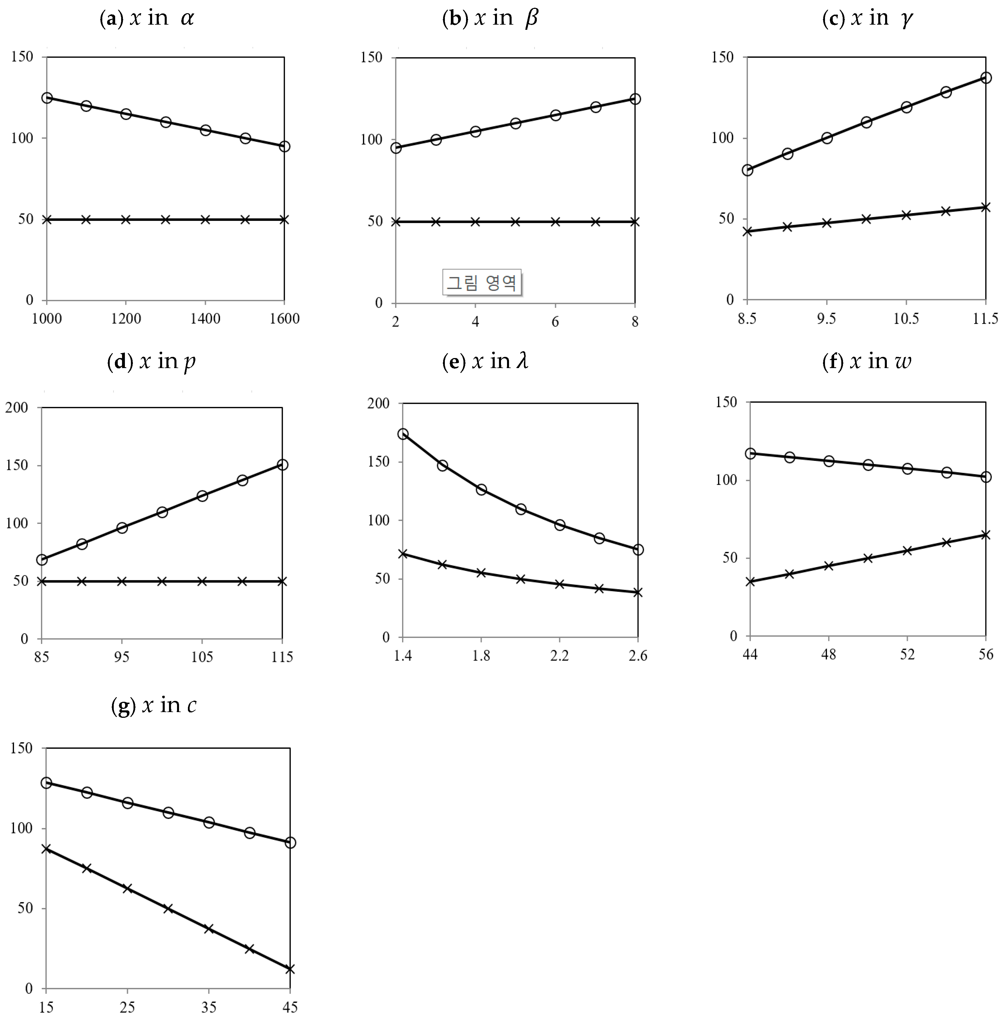
To investigate equilibrium behaviors according to changes in the business environment, we change the parameters within the following ranges. (1) External environment: demand potential $\alpha \in \left[1000, 1600\right]$, demand sensitivity to the market price $\beta \in \left[2, 8\right]$, demand sensitivity to environmental quality $\gamma \in \left[8.5, 11.5\right]$, and unit market price $p \in \left[85, 115\right]$. (2) Internal environment: magnitude of environmental quality investment $\lambda \in \left[1.4, 2.6\right]$, unit wholesale price $w \in \left[44, 56\right]$, and unit production cost $c \in \left[15, 45\right]$. The equilibrium behaviors of x, $I{R}_o$, $I{R}_c$, and IR with respect to the parameter changes are visualized in Figure 1, Figure 2 and Figure 3.

We summarize the implications of environmental quality as per Figure 1 as follows.

■

In the figure, we observe that the quantity incentive contract in Case Q always yields better environmental quality performance than the basic wholesale price contract in Case W, under any internal and/or external business conditions. Therefore, the OEM needs to consider the quantity incentive contract to enhance the supply chain’s sustainable development and properly respond to climate change.

■

In

Table 2. Effective business conditions for the environmental performance of the quantity incentive contract.

External Environment	Internal Environment
■ Demand potential α decreases ■ Demand sensitivity to price β increases ■ Demand sensitivity to environmental quality γ increases ■ Market price p increases	■ Environmental quality investment λ decreases ■ Wholesale price w decreases ■ Production cost c decreases

, we summarize the business conditions under which higher environmental quality is expected based on Figure 1.

Next, we investigate the equilibrium behaviors of profit improvement ratios shown in Figure 2 and Figure 3. The following is a summary of implications of Figure 2 and Figure 3.

■

The profit improvement ratios of the OEM, the CM, and the supply chain ($I{R}_o,$ $I{R}_c$, and IR) always show results greater than 0. Since the profit improvement ratios are defined as $I{R}_o=\frac{\left({П}_o^Q -{ П}_o^w\right) }{{П}_o^w}$, $I{R}_c=\frac{\left({П}_c^Q - {П}_c^w\right) }{{П}_c^w}$, and $IR=\frac{\left({П}^{Q }- {П}^w\right) }{{П}^w}$, they indicate that the quantity incentive contract in Case Q always yields better profit performance in any external and internal business environment compared to the basic wholesale price contract of Case W. That is, it is always guaranteed that ${П}_o^Q>{П}_o^w,$ ${П}_c^Q>{П}_c^w$, and ${П}^Q>{П}^W$ in these sensitivity analyses.

■

In any external or internal environment change, the change directions of $I{R}_o,$ $I{R}_c$, and IR are the same, as we can see in Figure 2 and Figure 3. This means that there is no choice problem for the OEM, whether depriving the profits of the CM and the entire supply chain for its own benefit or giving up its own profit for the long-term health of the entire supply chain. Both the OEM and the CM, as well as the whole supply chain, can have the motivation to adopt the quantity incentive contract voluntarily.

■

As similarly shown in Table 1, the effect of profit improvement is higher for the CM than for the OEM.

■

We summarize in

Table 3. Effective business conditions for the profit improvement with the quantity incentive contract.

External Environment	Internal Environment
■ Demand potential α decreases ■ Demand sensitivity to price β increases ■ Demand sensitivity to environmental quality γ increases ■ Market price p increases	■ Environmental quality investment λ decreases ■ Wholesale price w decreases ■ Production cost c increases

the situations in which we can expect higher profit improvement, based on the investigation of Figure 2 and Figure 3. In the external and internal business conditions listed in Table 3, we can expect better profit improvement from the quantity incentive contract.

■

Comparing the conditions in Table 2 and Table 3 and also the equilibrium behaviors with respect to the parameter changes in Figure 1, Figure 2 and Figure 3, we observe that the direction of change of the environmental quality and profit improvement ratios is the same in all cases except under one condition regarding production cost change. This reveals that investment in the sustainable development to improve environmental performance does not harm the profits of the entire supply chain or of individual players in most cases; however, there should be a careful, systematic assessment about the internal and external business conditions and their total impact on the supply chain’s overall performance.

In the above sensitivity analyses, the quantity incentive contract always results in better environment and profit performance for the OEM, the CM, and the entire supply chain compared to the basic wholesale price contract. However, we need to note that the quantity incentive contract cannot always be adopted, as shown in Proposition 2. For the quantity incentive factor to satisfy ${\epsilon }^{Q^{*}}>0$, the conditions in Proposition 2 must be satisfied, and once this condition is satisfied, ${\epsilon }^{Q^{*}}$ is always optimal; but if the conditions in Proposition 2 are not satisfied, the quantity incentive contract is not feasible. In this situation, we need to set ${\epsilon }^{Q^{*}}=0$, and then the quantity incentive contract becomes identical to the basic wholesale price contract. If we can get ${\epsilon }^{Q^{*}}>0$ by satisfying the conditions in Proposition 2, we can observe that the environmental quality is always enhanced compared to the basic wholesale price contract in Case W, and the profits of the OEM, the CM, and the entire supply chain are always better. Therefore, practicing managers should consider the quantity incentive contract as a viable option, but should also remain aware that the assessment of internal and external business conditions is prerequisite to the adoption of the quantity incentive contract, so as to guarantee its optimal performance. The conditions to obtain ${\epsilon }^{Q^{*}}>0$ in this numerical example are summarized in

Table 4. Range of parameters to adopt the quantity incentive contract in the numerical example.

External Environment	Internal Environment
■ Demand potential α < 2500 ■ Demand sensitivity to price β > 0 ■ Demand sensitivity to environmental quality γ > 6.3246 ■ Market price p > 78.1818	■ Environmental quality investment λ < 5 ■ Wholesale price w < 66 ■ Production cost c < 50

.

7. Concluding Remarks

In this paper, we considered an OEM–CM supply chain in which an OEM delegates product design and production to a CM. We dealt with the currently relevant issues of sustainable development and how to facilitate sustainable growth and properly respond to climate change. To do so, we considered an incentive strategy to better facilitate the CM’s investment in environmental quality and improve overall supply chain performance. Specifically, we examined the quantity incentive contract, incentivizing the CM’s investment in environmental quality based on the quantity sold to consumers. Then, we presented important implications by analytically comparing the quantity incentive contract with the basic wholesale price contract without any incentives that is commonly used in a typical supply chain, and conducted numerical experiments to gain better insights into the effectiveness and efficiency of the quantity incentive contract. The results of the investigation are summarized below.

First, this study reveals the conditions under which firms in the supply chain can adopt the quantity incentive contract. This contract is feasible when the OEM’s marginal profit is guaranteed above a certain level and when the CM’s decision on environmental quality has a certain level of impact on consumers’ buying behavior. Second, the quantity incentive contract can lead to a higher level of investment in environmental quality from the CM, and always yields better environmental quality, market, and profit performance compared to the basic wholesale price contract. Therefore, as environmental consciousness generates higher influence on consumers’ purchasing willingness, the quantity incentive contract proposed in our study becomes more suitable for improving the performance of not only individual members but also the overall supply chain in response to sustainability issues, including climate change. Third, the quantity incentive contract always enhances the overall profit performance not only of the CM and the entire supply chain but also of the OEM, which pays the incentive. These results can provide important insights for practicing supply chain managers who may be afraid of profit loss due to offering excessive incentives. Fourth, the quantity incentive contract is suitable to develop a long-term relationship between the OEM and the CM. With the quantity incentive contract, there is no such choice problem for the OEM—whether to reduce the profit of the CM for its own benefit or to give up its own profits for the long-term health of the supply chain. Therefore, both the OEM and the CM should be motivated to adopt the quantity incentive contract voluntarily. Fifth, we reveal the business conditions under which the quantity incentive contract becomes more effective in enhancing both environmental quality and overall profit performance: when the market shrinks, consumers become more sensitive to sales price or environmental quality, the market price increases, investment in environmental quality becomes more efficient, or the OEM’s bargaining power increases. Under any of these circumstances, it is recommended that the quantity incentive contract is adopted, not only to ensure higher environmental performance, but also to enhance the profit performance of the entire supply chain and each member.

Our study extends Yoo and Cheong [3], but the quantity incentive contract in this study yields different results from Yoo and Cheong [3] based on a one-time incentive scheme. Specifically, Yoo and Cheong [3] revealed the conditions under which the buyer needs to facilitate a one-time incentive contract, but they are different from the ones revealed in the present study. It means that there needs an extensive market research if a firm intends to adopt a particular incentive strategy. As environmental consciousness is regarded as an important impetus for consumers’ purchasing willingness in the contemporary market situation, the quantity incentive contract in this study can be a better alternative not only ensuring the environmental and profit performance of the entire supply chain but also enhancing a long-term relationship between the OEM and the CM.

Overall, we reveal that the quantity incentive contract can help enhance the environmental, market, and profit performance not only of the entire supply chain but also of the OEM and the CM specifically. By adopting the quantity incentive contract and offering the proper amount of incentive, the OEM can induce the optimal level of investment from the CM, not only to improve the environmental quality, for example, by reducing the amount of gas emissions or by enhancing the energy efficiency, but also to improve the supply chain’s overall profit performance. Moreover, we provide important implications revealing the unique characteristics of the quantity incentive contract, and offer necessary guidance for the adoption of the quantity incentive contract. Despite its contribution, however, this study is not free from limitations. One major limitation is related to contract type—we investigate only the quantity incentive contract in this study, but there exist many types of incentives in practice, and hence, there may be others that can better facilitate the supplier’s investment in environmental quality and, subsequently, better enhance overall performance. Therefore, future research should investigate other types of incentive contracts and compare the results with those of the present study.

References

- Quinn, J.B.; Hilmer, F.G. Strategic outsourcing. McKinsey Q. 1995, 1, 48–70. [Google Scholar]
- Lacity, M.C.; Willcocks, L.P. Global Information Technology Outsourcing: In Search of Business Advantage; Wiley: London, UK, 2001; 368p. [Google Scholar]
- Yoo, S.H.; Cheong, T. Quality improvement incentive strategies in a supply chain. Transp. Res. Part E. 2018, 114, 331–342. [Google Scholar] [CrossRef]
- Kaya, M.; Özer, Ö. Quality risk in outsourcing: Noncontractible product quality and private quality cost information. Naval Res. Logist. 2009, 56, 669–685. [Google Scholar] [CrossRef]
- Xie, G.; Yue, W.; Wang, S.; Lai, K.K. Quality investment and price decision in a risk-averse supply chain. Eur. J. Oper. Res. 2011, 214, 403–410. [Google Scholar] [CrossRef]
- Xie, G.; Yue, W.; Wang, S. Quality improvement policies in a supply chain with Stackelberg games. J. Appl. Math. 2014, 1–9. [Google Scholar] [CrossRef]
- Back, A.; Lee, J.-A.; Kok, C. Analysts Expect iPad to Give Lift to Asian Suppliers. The Wall Street Journal. 29 January 2010. Available online: http://www.wsj.com/articles/SB10001424052748704878904575030633950504718 (accessed on 22 November 2018).
- Choi, S.-J. Cosmetics Makers Advance to Global Markets on ‘K-Beauty’ Boom. KoreaTimes. 16 October 2016. Available online: https://www.koreatimes.co.kr/www/news/biz/2016/10/123_216150.html (accessed on 10 December 2018).
- Yuan, B.; Gu, B.; Guo, J.; Xia, L.; Xu, C. The optimal decisions for a sustainable supply chain with carbon information asymmetry under cap-and-trade. Sustainability 2018, 10, 1002. [Google Scholar] [CrossRef]
- Reeves, R. On a (Leftish) wing and a prayer? Religion is a dirty word in British politics but a faith system that emphasised social good might be better than today’s uncritical worship of the market. Eur. J. Oper. Res. 2015, 242, 1017–1027. [Google Scholar]
- Yu, Y.; Han, X.; Hu, G. Optimal production for manufacturers considering consumer environmental awareness and green subsidies. Int. J. Prod. Econ. 2016, 182, 397–408. [Google Scholar] [CrossRef] [Green Version]
- Chen, J.; Hu, Q.; Song, J.S.J. Contract Types and Supplier Incentives for Quality Improvement. Available online: https://papers.ssrn.com/soL3/papers.cfm?abstract_id=2608772 (accessed on 26 June 2019).
- Toptal, A.; Özlü, H.; Konur, D. Joint decisions on inventory replenishment and emission reduction investment under different emission regulations. Int. J. Prod. Res. 2014, 52, 243–269. [Google Scholar] [CrossRef]
- Yalabik, B.; Fairchild, R.J. Customer, regulatory, and competitive pressure as drivers of environmental innovation. Int. J. Prod. Econ. 2011, 131, 519–527. [Google Scholar] [CrossRef]
- Marufuzzaman, M.; Ekşioğlu, S.D.; Hernandez, R. Environmentally friendly supply chain planning and design for biodiesel production via wastewater sludge. Transp. Sci. 2014, 48, 555–574. [Google Scholar] [CrossRef]
- Bertarelli, S.; Lodi, C. Heterogeneous firms, exports and Pigouvian pollution tax: Does the abatement technology matter? J. Clean. Prod. 2019, 228, 1099–1110. [Google Scholar] [CrossRef]
- Liu, Z.L.; Anderson, T.D.; Cruz, J.M. Consumer environmental awareness and competition in two-stage supply chains. Eur. J. Oper. Res. 2012, 218, 602–613. [Google Scholar] [CrossRef]
- Luo, Z.; Chen, X.; Wang, X. The role of co-opetition in low carbon manufacturing. Eur. J. Oper. Res. 2016, 253, 392–403. [Google Scholar] [CrossRef] [Green Version]
- Zhu, W.; He, Y. Green product design in supply chains under competition. Eur. J. Oper. Res. 2017, 258, 165–180. [Google Scholar] [CrossRef]
- Klassen, R.; Vachon, S. Collaboration and evaluation in the supply chain: The impact on plant-level environmental investment. Prod. Oper. Manag. 2003, 12, 336–352. [Google Scholar] [CrossRef]
- Green, K.W., Jr.; Zelbst, P.; Bhadauria, V.; Meacham, J. Do environmental collaboration and monitoring enhance organizational performance? Ind. Manag. Data Syst. 2012, 112, 186–205. [Google Scholar] [CrossRef]
- Ji, J.; Zhang, Z.; Yang, L. Comparisons of initial carbon allowance allocation rules in an O2O retail supply chain with the cap-and-trade regulation. Int. J. Prod. Econ. 2017, 187, 68–84. [Google Scholar] [CrossRef]
- Chen, X.; Wang, X.; Zhou, M. Firms’ green R&D cooperation behavior in a supply chain: Technological spillover, power and coordination. Int. J. Prod. Econ. 2019, 218, 118–134. [Google Scholar]
- Ghosh, D.; Shah, J.A. Comparative analysis of greening policies across supply chain structures. Int. J. Prod. Econ. 2012, 135, 568–583. [Google Scholar] [CrossRef]
- Xu, X.; He, P.; Xu, H.; Zhang, Q. Supply chain coordination with green technology under cap-and-trade regulation. Int. J. Prod. Econ. 2017, 183, 433–442. [Google Scholar] [CrossRef]
- Shi, X.; Chan, H.L.; Dong, C. Value of bargaining contract in a supply chain system with sustainability investment: An incentive analysis. IEEE Trans. Syst. Manag. Cybern. 2018, 9, 1–13. [Google Scholar] [CrossRef]
- Starbird, S.A. Penalties, rewards, and inspection: Provisions for quality in supply chain contracts. J. Oper. Res. Soc. 2001, 52, 109–115. [Google Scholar] [CrossRef]
- Baake, P.; von Schlippenbach, V. Quality distortions in vertical relations. J. Econ. 2011, 103, 149–169. [Google Scholar] [CrossRef] [Green Version]
- Schmitz, P.W. Allocating control in agency problems with limited liability and sequential hidden actions. RAND J. Econ. 2005, 36, 318–336. [Google Scholar]
- Karmarkar, U.S.; Pitbladdo, R.C. Quality, class, and competition. Manag. Sci. 1997, 43, 27–39. [Google Scholar] [CrossRef]
- Banker, R.D.; Khosla, I.; Sinha, K.K. Quality and competition. Manag. Sci. 1998, 44, 1179–1192. [Google Scholar] [CrossRef]
- Zhang, L.; Zhou, H.; Liu, Y.; Lu, R. Optimal environmental quality and price with consumer environmental awareness and retailer’s fairness concerns in supply chain. J. Clean. Prod. 2019, 213, 1063–1079. [Google Scholar] [CrossRef]
- Cachon, G.P. Supply chain coordination with contracts. In Handbooks in Operations Research and Management Science—Supply Chain Management: Design, Coordination and Operation; De Kok, A.G., Graves, S.C., Eds.; Elsevier: Amsterdam, The Netherlands, 2003; Volume 99, pp. 229–340. [Google Scholar]
Figure 1.
Environmental quality of Cases Q and W (○: Case Q, ×: Case W).
Figure 2.
Profit improvement ratio of Case Q in the external business environment.
Figure 3.
Profit improvement ratio of Case Q in the internal business environment.