Optimizing Incentive Policy of Energy-Efficiency Retrofit in Public Buildings: A Principal-Agent Model

1
School of International and Public Affairs, Shanghai Jiao Tong University, Shanghai 200240, China
2
Department of Building and Real Estate, Hong Kong Polytechnic University, Hong Kong, China
3
School of Economics and Management Engineering, Beijing University of Civil Engineering and Architecture, Beijing 100037, China
*
Author to whom correspondence should be addressed.
Sustainability 2019, 11(12), 3442; https://doi.org/10.3390/su11123442
Submission received: 24 May 2019
/
Revised: 17 June 2019
/
Accepted: 18 June 2019
/
Published: 22 June 2019
(This article belongs to the Section Energy Sustainability)
Abstract
:The building sector consumes most energy in the world, especially public buildings, which normally have high energy-use intensity. This phenomenon indicates that the energy-efficiency retrofit (EER) for public buildings is essential for energy saving. Incentive policies have been emphasized by governments in recent years, but their effectiveness has not been sufficient. A major reason is agency problems in EER and that the government and building owners have asymmetric information. Furthermore, most policies apply identical standard to existing buildings of different types, resulting in resistance from owners and tenants. To mitigate this issue, this study proposes a principal–agent model to optimize incentive policy in EER. The proposed model defines two pairs of principal–agent relations (i.e., the government-owner and owner-tenant) and models their behaviors under different scenarios as per principal–agent theory. The results indicate the optimal incentive policies for different scenarios. In addition, critical factors of policy making, such as cost, risk, uncertainty, and benefit distribution are discussed. This study has implications for policy that will benefit policy makers, particularly in promoting EER by mitigating the agency problem found for the different scenarios.
1. Introduction
Nearly 40% of energy is consumed by the building sector globally, which has led to remarkable air pollution and health risk [1]. Compared to residential buildings, public buildings have much higher energy-use intensity [2]. For a public building, more than 80% of life-cycle energy use is consumed after the building is occupied [3]. Therefore, an energy-efficiency retrofit (EER) is a promising means of energy saving in public buildings which has attracted more attention in recent years [4,5,6,7,8].
Governments all over the world have emphasized policies for EER in public buildings [9,10,11,12]. For example, in China, pilot EER projects included 60 million m2 of public buildings according to the 12th Five-Year Plan (2011–2015) [13]. Although the target areas of EER were finally achieved, most pilot project were state-owned buildings; they included hospitals, schools and government offices [14]. The EER target was achieved because of administrative pressure rather than market-oriented economic measures. A major reason is that the incentive policies of the government cannot effectively inspire building owners to take the initiative on EER [15,16].
Numerous studies have tried to explain why incentive policy is ineffective when it comes to EER [14,17,18,19,20]. Alam, Zou, Stewart, Bertone, Sahin, Buntine and Marshall [10] indicated that a lack of political will and financial support are key barriers to EER policy. Bertone et al. [21] emphasized that financial mechanisms is an important factor impacting the effectiveness of policy. Kasivisvanathan et al. [18] indicate that incentives by government could not match the building owner’s cost, and also the long payback period (normally more than five years), making it difficult for EER projects to generate economic benefits. Liu et al. [22] argued that the level of public participation will also influence the effectiveness of EER policy. Furthermore, the government incentive is mainly on the basis of the energy performance after EER, however, the climate, building condition, occupier activities in a building, and other uncertain factors could influence the energy performance of a building [17,19,20,23,24,25].
Several pilot studies have attempted to address these problems of incentive policy in EER. Although some studies analyzed the relationship between government and building owners [10,23,26,27], the agency problem in EER has not been effectively addressed [28]. First, the government and building owners are information asymmetric in that building owners have more information about EER. How to design an optimal policy to encourage building owners and achieve maximum effect is a typical agency problem. In addition, there is also an agency problem between building owners and tenants—a typical problem in public buildings. Another problem is that different building conditions can significantly influence the decisions of owners and occupiers in EER (e.g., occupied types, allocation of energy-saving benefits) [29]. Therefore, a narrow analysis without considering building conditions in EER may lead to inaccurate results and ineffective policy.
To bridge the research gaps, this study develops a novel principal-agent model for optimizing incentive policies under different scenarios in EER. This study differs from most previous empirical studies. Instead of investigating decision-making behaviors through a survey, it analyzes the stakeholders’ behaviors as per principal–agent theory. Because interviewees tend to show positive attitude to energy saving and sustainability, the survey results normally have an optimistic bias. Therefore, this study models the stakeholders’ decisions under different scenarios based on principal–agent theory. This method is an effective approach to reveal the mechanism of stakeholders’ decisions in EER and provide policy implications for the government.
2. Methodology
2.1. Principa–Agent Theory
Agency problems are common in reality, in that the agent represents the principal to implement works or make decisions. For example, patients and doctors, clients and lawers are typical pincipal-agent relations. There are two key issues in agency problem, split incentive and asymmetric information [30]. Split incentive indicates both pincipal and agent want to maximze their own utility, so the aims of them are normally different. Asymmetric information means agents normally have more information than principals, that agents can use this to persue their own interests and may harm the interests of principal. It is impossible or very difficult for the principal to supervise the agent’s real action.
Principal–agent theory was introduced to address agency problems. It defines an optimized contract, that can induce agent’s effort and maximize principal’s utility. In fact, the principal-agent theory is essentially to solve an optimization problem [30]. In the environmental research area, principal–agent theory has been used in some case studies, for example the energy utility regulation, and energy-efficiency decisions in the trucking and shipping industry [31,32,33].
In this study, there are two pairs of principal–agent relations (i.e., the government and building owners, the building owners and tenants) that should be considered in EER policy design. Accordingly, a model based on the principal–agent theory was developed to optimize incentive policy in EER. The problem can be specified to design the optimal incentive by the principals (government/owner) to maximize the efforts of agents (owner/occupier) and the utilities of principals. The detailed model description is illustrated in Section 2.2.
2.2. Model Description
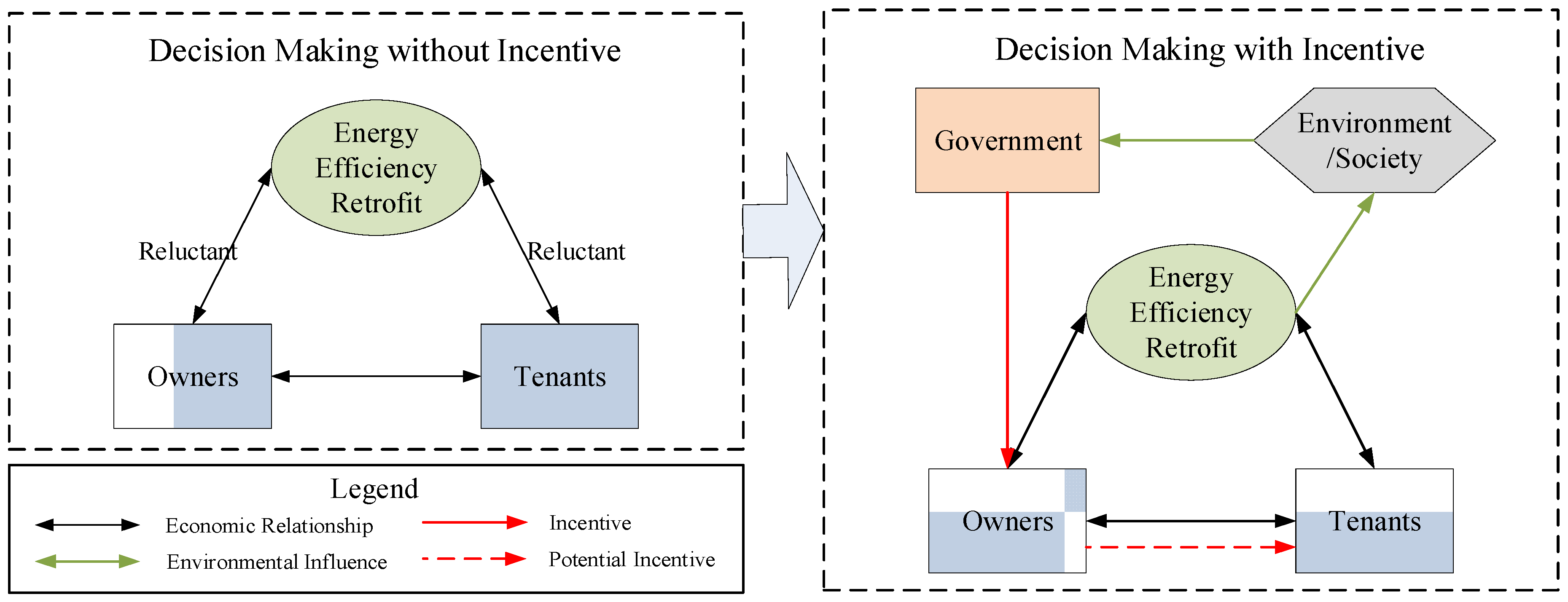
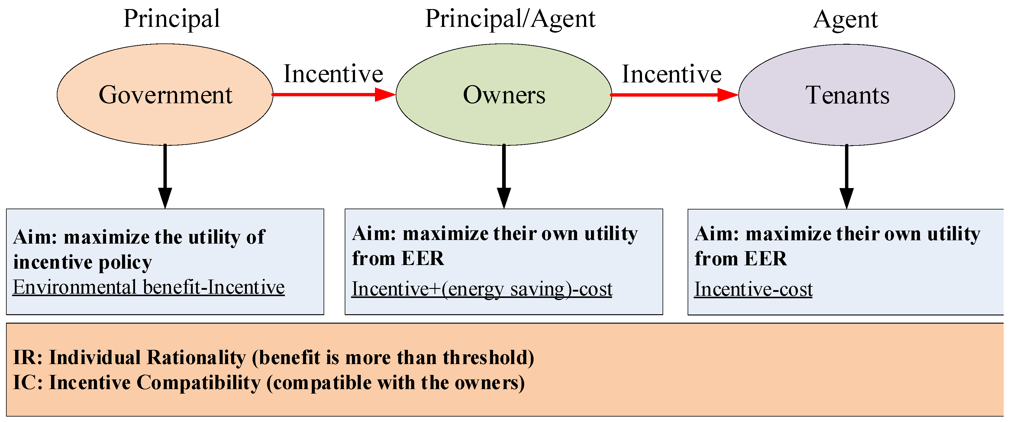
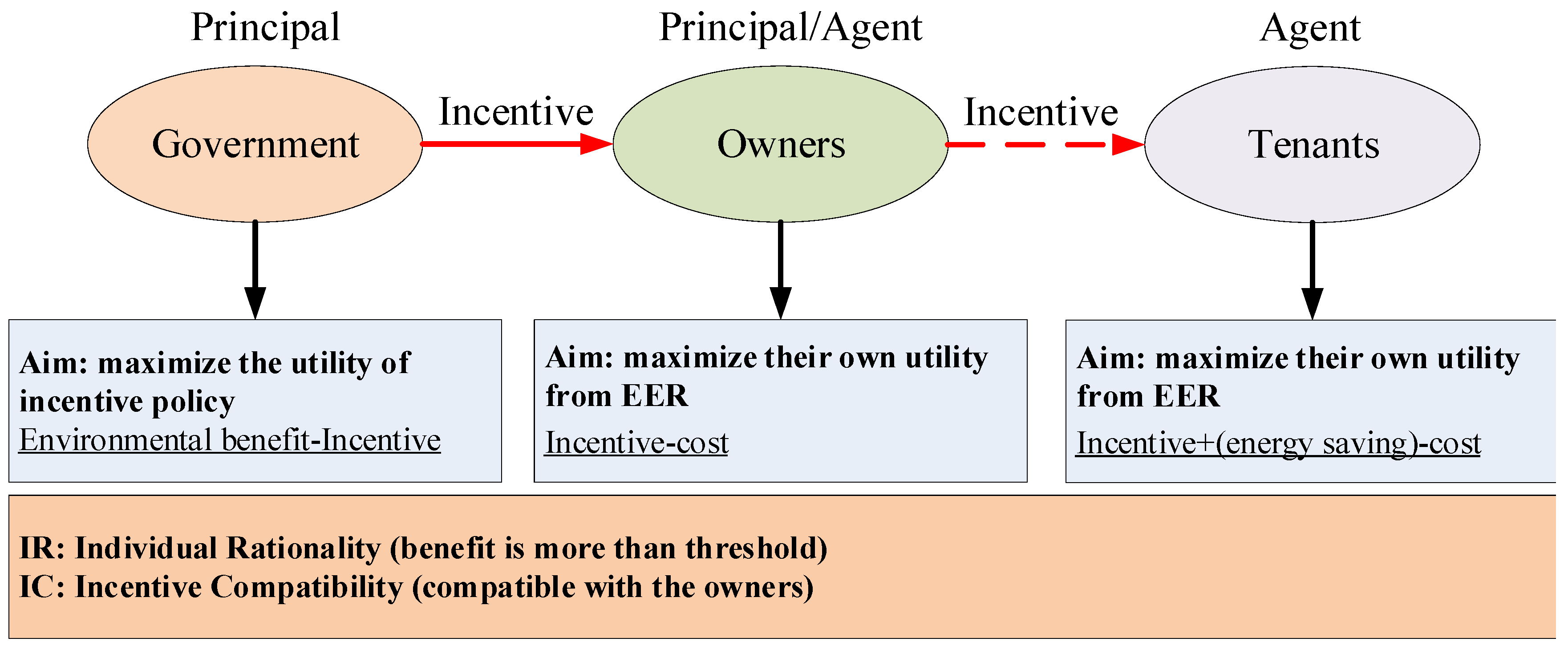
EER can bring a large amount of environmental benefits and social welfare, however these social benefits are not considered as a high priority by individuals (i.e., building owners and tenants). Liang, Peng and Shen [29] analyzed the relationship between owners and tenants in EER based on the game model, and indicated that due to split interests, both owners and tenants would be reluctant to begin an EER without government incentives. This result explains why most promotions of ER have not received active responses in industry. Thus, the government needs to give incentives to relocate the benefit and cost, which can promote EER through an economic lever.
When there is no incentive, the interest relationship between owners and tenants is shown in the dashed box on the left of Figure 1. When the government joins and provides incentives, the relationship among stakeholders is changed, as shown in the dashed box on the right of Figure 1. The government can evaluate the environmental benefits and social welfare of an EER project (shown by green lines in Figure 1), and give appropriate incentives to the owner of the building (shown by the red line in Figure 1). The owners can gain more benefits through government’s incentive. When there are satisfied benefits from EER, they will initiate EER. If a building is not owner-occupied, the owner needs to negotiate with the tenants and may give incentives to balance the cost of EER (shown by the dashed red line in Figure 1). Then, the owners and tenants can cooperate on EER. Therefore, an appropriate incentive is essential for promoting EER.
Therefore, the main problem can be defined as how to make an optimal incentive policy that can maximize the efforts of owners and tenants for EER. To address this problem, a principal–agent model is developed to optimize the incentive policy and balance the benefits and costs for the three stakeholders (i.e., owners, tenants, and government).
2.2.1. Players in the Principal–Agent Model
There are various stakeholders involved in EER [34,35,36]. However, in the initial phase of EER, three stakeholders (i.e., government, building owners, and tenants) play the most essential roles in public buildings [29]. The current study attempts to identify the optimal incentive for EER in public buildings through a principal–agent model. Accordingly, our model focuses on the two pairs facing agency problems, that is, government and building owners, as well as building owners and tenants.
Government versus building owners: The government gives incentives to building owners to encourage them to participate and make more efforts on EER. However, they have asymmetric information and split incentives. First, the government does not know the efforts of building owners want to pay on EER. Further, the objectives of them are different. The government’s objective is to optimize the effect of EER, but the owners’ objective is to pursue their own benefits from EER. Therefore, there is a typical agency problem regarding how to design an optimal incentive by government to gain the best retrofit results.
Building owners versus tenants: For the tenant occupied buildings, if the tenants do not gain enough benefits and are reluctant to undertake EER, building owners should give them incentives to influence their decision making on EER. However, the building owners does not have the complete information of the tenants. In addition, the objective of them are different, both of them aim to maximize their own benefits from EER. Therefore, there is also an agency problem between them, which is how to design an optimal incentive by building owners to gain the best retrofit results.
It is worth noting that in real EER projects, since each owner is independent, the government has to communicate with each owner individually. But because the owners have similar aims and interests, their decision-making behavior will not be significantly different in the same scenario. Therefore, building owners are considered homogeneous in the model. Similar to the owners, although the occupiers are independent in reality, they are abstract to an identical entity in the model.
2.2.2. Benefits and Costs
The benefits and costs of stakeholders in the principal–agent model are listed in Table 1. The benefits of owners are economic benefits from the retrofit and incentives from the government, while the costs of owners are the cost of EER and incentives to tenants. The benefits of tenants are economic benefits from the retrofit and incentives from owners, while the costs of tenants are the cost of EER. The benefit of government is the environmental and social benefits, while the cost is the incentives to owners. The incentive from owners to tenants is optional, depending on the relationship between them.
2.2.3. Scenarios
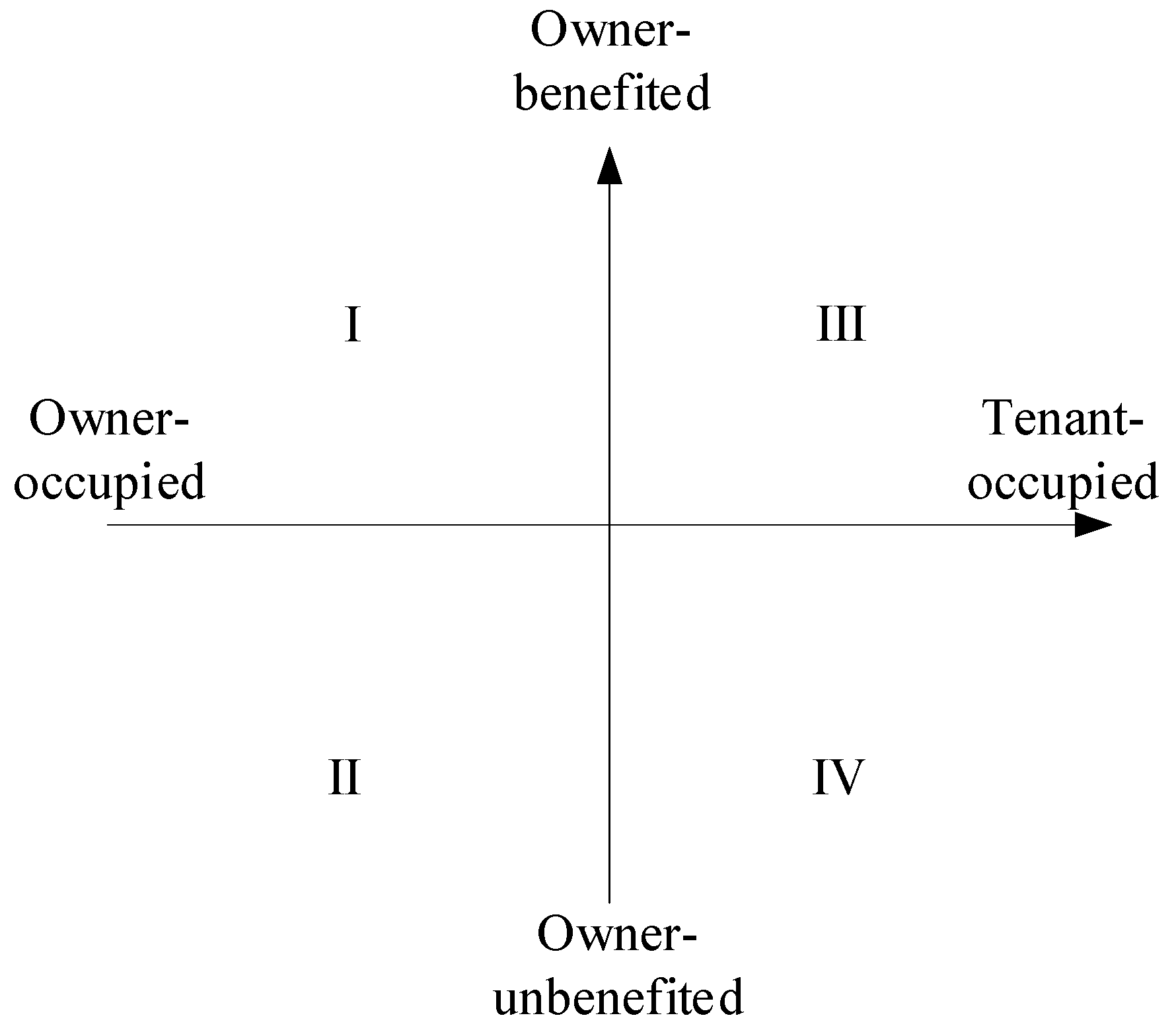
Interest relationships between owners and tenants vary according to different situations. Based on the type of occupied building and whether owners can benefit from EER, there are four scenarios, as shown in Figure 2.
The scenarios are classified by two criteria, one is occupancy type and the other is beneficiary of energy bill saving. The latter is straightforward in that who can gain benefit from energy saving will have more initiatives for EER. It will influence the optimal incentive by government. For example, if the building owner cannot benefit from energy bill saving, the government should provide more incentive to let the owner participate in EER. Numerous previous studies have indicated this point [24]. Occupancy type is another important factor influencing incentive policy. In the owner-occupied building, the owner can make a decision on EER. In the tenant-occupied building, the owner has to communicate and negotiate with tenants, which make the decisions of EER more complex. The government or building owner need to give some compensation to tenants to promote EER. The occupancy type is also highlighted as an important factor influencing decision making of EER by a number of previous studies [29].
The four scenarios are introduced in detail as follows.
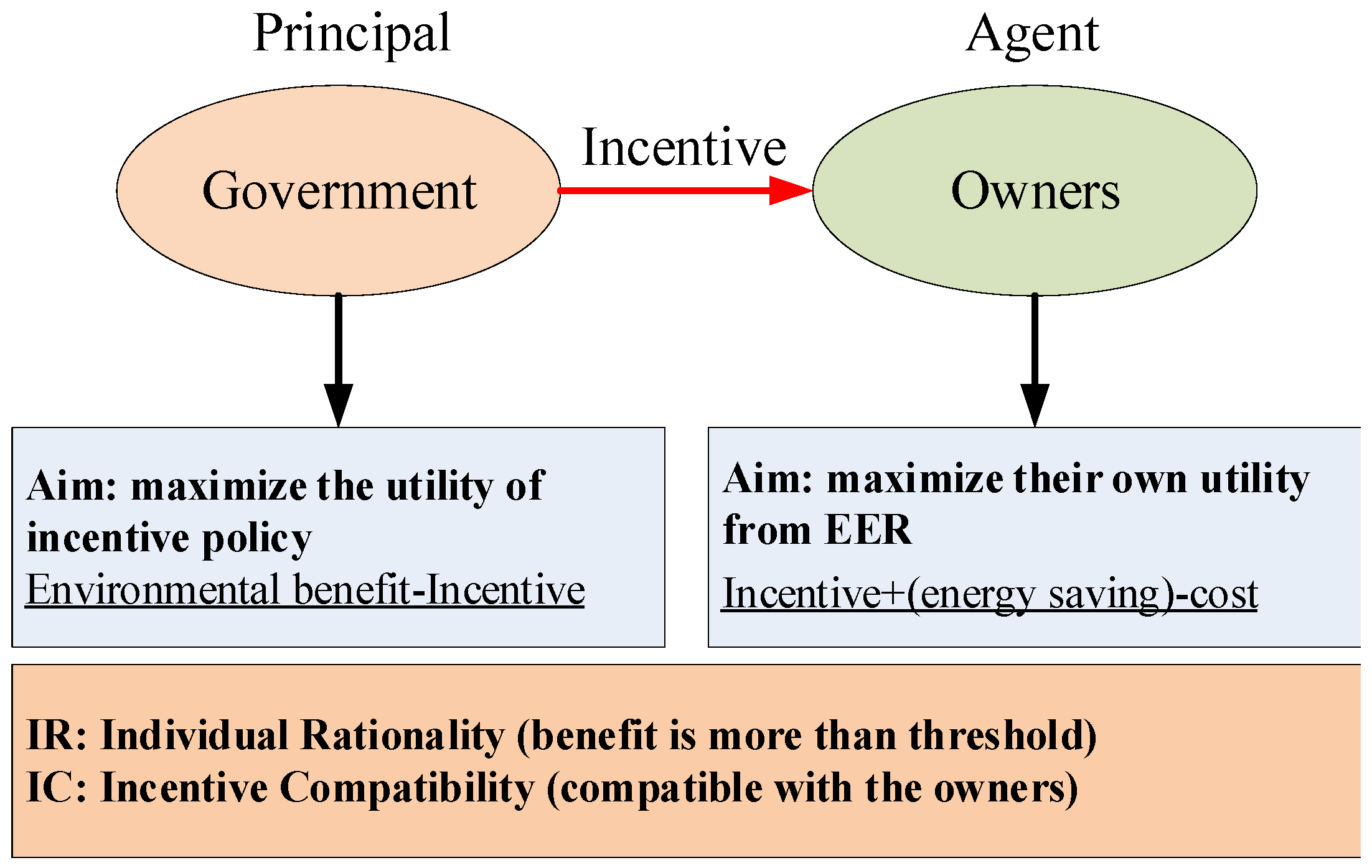
Scenario I: represents the owner-occupied and owner-benefitting buildings. The buildings are occupied by the owners of the buildings and they pay the utility bills themselves; thus, the owners can gain benefits from EER by energy saving. Typical buildings in Scenario I are the headquarters of companies and institutes. For example, the headquarters building of China Resource Group in Hong Kong is a self-owned property. The building was completed in 1983 and has been retrofitted several times. The company can benefit from the EER. The property manager mentioned that the retrofit of an elevator saved on the energy bill significantly and also improved the delivery efficiency. The principal-agent model in Scenario I is shown in Figure 3.
As shown in the conceptual model in Figure 3, the government is the principal and the building owner is the agent. The government (principal) delegate building owner (agent) to implement EER. The government aims to maximize the utility of EER, but owners aim to maximize its own benefit. To encourage more efforts on EER and gain more utilities, the government gives incentives to building owners. The problem is how to optimize the incentive by the government. In the principal–agent model, there are normally two constraints [30]. One is the individual rationality constraint (IR), that the agent’s benefit should be more than a threshold. The other one is the incentive compatibility constraint (IC), that the optimal strategies of principal and agent should be compatible.
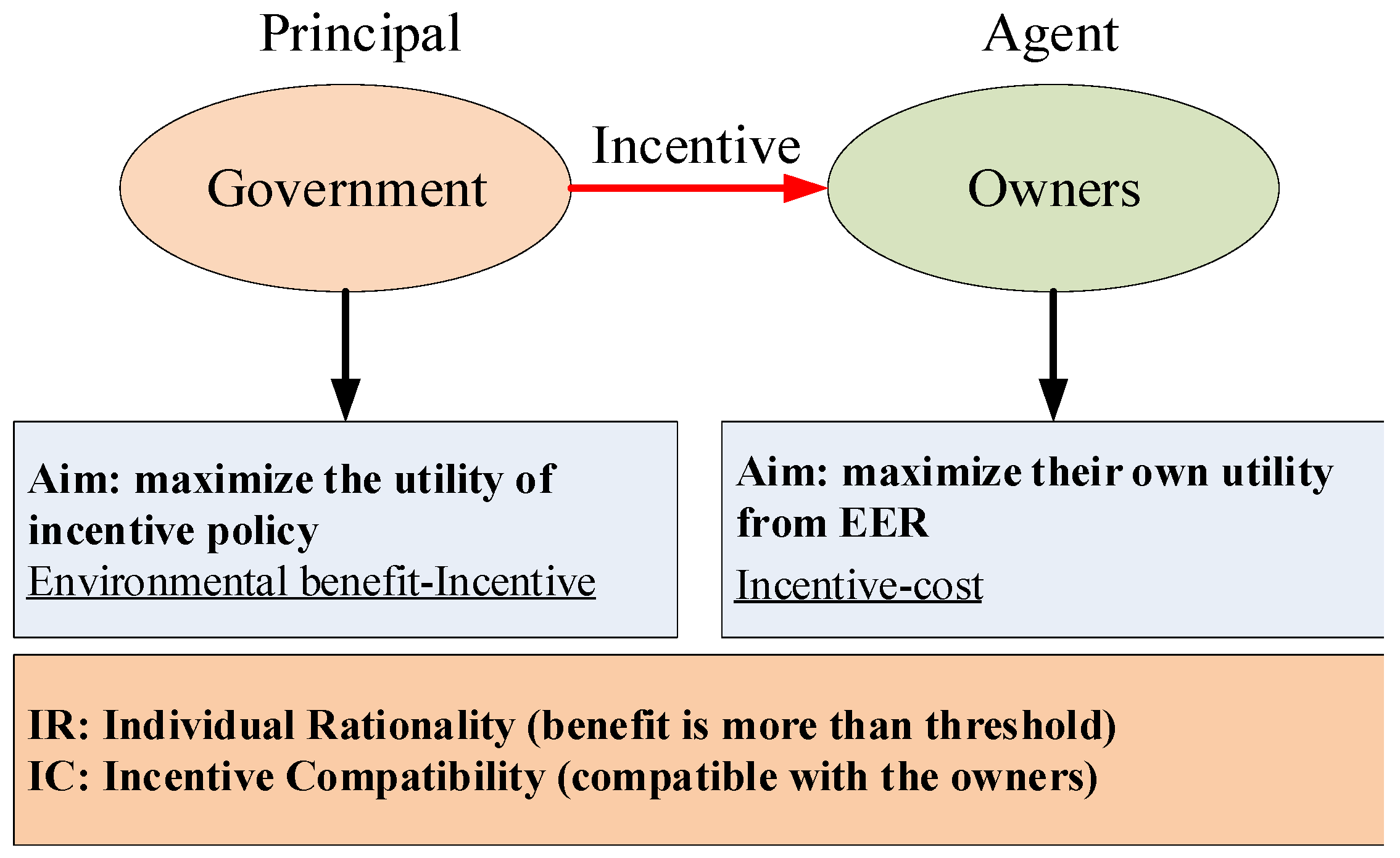
Scenario II: represents the fact that the buildings are owner-occupied, but the owner does not benefit from savings. The buildings are occupied by the owners, but the utility bills are paid by public finance. Hence, the building owners cannot gain the benefits from EER. Typical buildings in Scenario II are government and public buildings. One case is the city hall in Shenzhen. The government pays the energy bills of city hall. The operation managers stated that the building implemented EER only because of administrative orders. Since the revenue and expenditure are separate in this kind of state-owned building, the EER cannot bring benefit of energy bill saving for them but may lead to some risks. Therefore, they do not have an incentive for EER. The principal–agent model in Scenario II is shown in Figure 4.
As shown in Figure 4, the aim of the principal and agent are the same as that in Scenario I. The difference is that owners’ benefits do not include energy savings. That means the owners’ benefits should be less than that in Scenario I, which, in turn, will influence the optimal incentive by the government.
Scenario III: represents the tenant-occupied and owner-benefitting buildings, which are the leased commercial buildings where the owners pay the utility bills. Since the owners pay the utility bills, they can gain energy-saving benefits from EER. Typical buildings in Scenario III are shared offices. One case is Wework in Shanghai. The business model of Wework is renting office space by headcount (around 2000 CNY per person per month). All the energy bills and other expenditures are included in the rent. Therefore, the tenant does not need energy bills and also cannot gain benefit from energy saving by EER. The principal–agent model in scenario III is shown in Figure 5.
As shown in Figure 5, tenants are joined in this scenario. There are two pairs of principal-agent relationship in this model, one is the government and building owners, and the other one is building owners and tenants. The aim of tenants is to maximize their own benefit in EER. Since tenants cannot gain energy-saving benefits from EER, the owners should provide compensation to incentive tenants give efforts to retrofit, the benefit of tenants can be defined as incentive by owners minus the retrofit cost.
Scenario IV: represents the tenant-occupied and owner-unbenefited buildings, normally the leased commercial buildings where the tenants pay the utility bills. Most commercial buildings, including office buildings and shopping centers, are in this scenario. For example, the tenants in shopping centers normally have to pay energy bills by themselves. Therefore, they can have direct benefit from energy saving by EER. The tenants can gain energy-saving benefits from EER.
As shown in Figure 6, the tenants’ aim is the same as that in Scenario III. Since the tenants can gain benefits from energy saving, this incentive for owners is optional, depending on the situations of the retrofit. If there are incentives for owners, the benefit of tenants can be defined as an incentive for owners plus energy saving minus the retrofit cost; otherwise, the benefit of tenants can be defined as an incentive by owners minus the cost.
2.2.4. Variables
This study defines four types of variables in the model (i.e., dependent, independent, intermediate and data), shown in Table 2.
In this model, the independent variable is incentive, including both government’s incentive and owner’s incentive. The independent variable is utility. The essential issue is to find an appropriate incentive to maximize the utility. Because the incentive does not act on utility directly, the intermediate variables are introduced in the model. The incentive can influence the income and cost of owners and tenants, and then influence their efforts on EER, and finally influence the effect of EER and utility of the government. Therefore, the income, cost, benefit and effort are intermediate variables. The fourth is data, which means these variables can be defined from the existing data. For example, the exogenous uncertainty probability distribution θ depends on climate, technology development, condition of the existing building, etc. The coefficient of owner’s cost depends on the technology development, material price, condition of the building, etc. These variables can be estimated based on the data of previous EER projects.
On the basis of the aforementioned problem definition, the relation among owners, tenants, and government can be analyzed with the principal–agent theory. The most efficient incentive can be identified and the optimal actions of each stakeholder can, accordingly, be proposed. The derivations and results are illustrated in the following section.
3. Results
3.1. Preparatory Work
EER can bring environmental benefits , which depend on the owners’ efforts and exogenous uncertainty θ [16]. If owners put in more effort on EER, they will gain more environmental benefits from EER. θ indicates the uncertainty of the exogenous environment (e.g., technology development, climate changes and interdisciplinary collaboration) [19]. can be calculated by Equation (1):
EER can also bring economic benefits (e.g., higher rents, higher occupied rate) [37,38]. Similar to environmental benefit, can be calculated by Equation (2):
It is worth noting that the energy price is a static constant (not variable) and implicit in coefficient . This study focuses on incentive policy in the short term, so the energy price is stable. In addition, EER is mainly related to electricity price (oil, gas and other energies are not common in public buildings), and electricity price is relatively stable. For example, the fluctuation of electricity price for public buildings is only around 0.06 CNY (0.0087 USD) in the last five years in Shanghai, China. Therefore, the energy price in EER is considered as a constant in this study.
The government give an incentive to pursue better EER effect, therefore the government’s incentive should be proportional to the environmental benefit of EER, given by . Namely the higher environment benefit government can have, the more incentive the government wants to pay. Owing to exogenous uncertainty, even when owners focus on EER, the effect may not be positive. Therefore, a constant is defined to ensure that the incentive policy is optimal to exogenous uncertainty. This incentive expression is shown in Equation (3). is the coefficient on the incentive, which indicates the redistribution of benefits from EER. The higher this coefficient, the more incentives to the similar EER results [37]. Specifically, the owners can get more benefits from EER, while the government gets less benefit from EER.
For the building owners who carry out EER, their incomes is the economic benefits (e.g., energy cost savings, incentives by government) plus minus the costs of EER. The incomes of tenants from EER can be defined as the benefits (e.g., energy cost savings, incentive by building owner) minus the cost of EER. and in the four scenarios are shown in Table 3.
The cost of the owner can be defined in Equation (4), where is the cost coefficient. The cost of tenant can be defined in Equation (5), where is the cost coefficient. The cost function is convex, and their marginal cost will increases when owners pay more efforts on EER. It follows the law of diminishing marginal returns [39].
represents the utility of government gains from EER. The better effect of EER, the more the benefits that the government can obtain [40]. The government is considered as risk neutral in this study, then the utility function can be expressed in Equation (6).
The expectation of government utility is shown as the certainty equivalent in Equation (7).
and is the owner’s and tenant utility function, which indicates the owner’s and tenant’s satisfaction degree from EER respectively [41]. This study assumes that both owner and tenant have absolute risk aversion [29,35]. It means if the owner and tenant are more risk averse, they will be more cautious and do not want to make efforts on EER [35]. The utility function and with risk aversion are illustrated in detail in Appendix A.
To mitigate the agency problem in EER, the principal (government) has to design the optimal incentive to induce more agent’s (owner’s) efforts on EER that can optimize the principal’s utility. The principal–agent model is to solve the optimization problem under individual rationality constraint (IR) and the incentive compatibility constraint (IC), shown in Equation (8).
s.t.
IR and IC are satisfied.
The specific mathematical definition and deduction are illustrated in Appendix A.
3.2. Results of Optimal Incentives in the Four Scenarios
By solving the optimization problem in the previous section, the optimal incentives and efforts for the four scenarios are summarized in Table 4. These results are for the assumption that tenants are risk averse. If tenants are risk neutral, namely, , the results in Table 3 can be simplified, as shown in Table 5.
4. Discussion
4.1. Scenario I Versus Scenario II
First, it is worth noting that this result of is not in line with common sense. It is generally assumed that incentive should be higher when the building owner cannot gain saving on an energy bill. However, according to the proposed principal-agent model, has the same value in Scenarios I and II in Table 2. It indicates that whether or not owners can gain benefits from EER, the government incentives should be the same in Scenario I and II.
Second, under the same incentive coefficient , . is proportional to , , and , which means the higher the economic benefit coefficient, environmental benefit coefficient, and government incentives, the higher the efforts owners will make. It indicates that technology development is very important since it can induce more owner efforts because and can be improved. Accordingly, is negatively correlated with . This correlation means the higher the cost coefficient of EER, the lower the efforts owners make. Given that high costs improve the difficulty of EER, it will cause the reluctant attitude of owners. According to the results, the government can consider improve technology development and reduce cost of EER, which will improve the efficiency of the incentive significantly.
4.2. Scenario III versus Scenario IV
First, , and the difference between the of the two scenarios is . It indicates how much an owner should pay to optimize tenants’ efforts when tenants cannot get the economic incomes from EER.
For the owner, under the same incentive coefficient , . But for the tenant, under the same incentive coefficient, . This indicates the incentive should balance the economic incomes of owner and tenant to optimize the efforts of both. The difference between the of the two scenarios is . When tenants are risk-neutral, the difference is zero, , which means the owner does not need pay extra compensation for the tenant. Otherwise, if , the difference will also approach zero.
4.3. Government Incentive
According to the results in Scenario I and II, the higher the cost coefficient on EER, risk aversion, and uncertainty, the higher the incentives government should provide. As is a factor representing the risk allocation between government and owner, it follows that if is lower (namely, the cost coefficient on EER, degree of risk aversion, or uncertainty is higher), then owners will want to undertake fewer risks. is negatively correlated with . A higher means the government can easily get environmental benefits from EER, and so it does not need to provide high compensation.
It is worth noting that the government incentive is not related to the risk attitude In Scenario III. Regardless of whether the tenant is risk averse or neutral, the incentives are the same. is only related to . Assuming that , there are only incentives, without any punishment. Hence, , which indicates that only when the environmental benefit of EER is higher than the economic benefit will it be rational for the government to give incentives.
is much more complex in Scenario IV than in the previous three scenarios. depends on the value of , and . However, in reality, most commercial buildings belongs to Scenario IV. This is why policies for EER are difficult to launch and have not achieved satisfactory effects. Therefore, analyzing the relation between owners and tenants is essential for policy making for EER. One case is the Baima Clothing Building in Guangzhou, China, a clothing wholesaler. Although the building is state owned, it still has not started EER yet. The main reason is there are more than 1000 tenants (shop of each tenant is very small). The facility managers indicated that the government ordered an EER, but it is too difficult to balance the benefits of numerous tenants. Therefore, the EER plan aborted finally. Previous incentive policy by government only focused on building owners. Future policy should pay more attention on tenants, especially in condition of Scenario IV.
4.4. Efforts of Owners and Tenants
Under the same incentive coefficient , , which means no matter whether buildings are owner-occupied or tenant-occupied, owners will pay the same efforts when they can get incomes from EER.
is proportional to and . This correlation indicates the higher the economic benefit coefficient and owner incentives, the higher the efforts tenants will make. Given that is positively correlated with , is also positively correlated with . Additionally, because of its positive correlation with , is also negatively correlated with , and . This correlation means the higher the cost coefficient of owners and tenants, the risk averse, and the uncertainty, the lower the efforts tenants make. Given that high costs and uncertainty improve the difficulty of EER, it will cause a reluctant attitude among tenants. Therefore, besides incentives, the government should pay more attention to reducing costs and uncertainty of EER that can improve the tenant’s effort significantly.
4.5. Risk
If all stakeholders are risk neutral, namely, , then . This result indicates that owners will face more risks and gain more benefits from EER compared to a risk-averse condition. A constant means the government’s incentives should be not related to the external environment variables, and the sharing of risks between government and owner is a constant.
in Scenario I, II, and III is the same under different risk preferences because it is not correlated with . This non-correlation indicates that the risk preference does not affect owners’ efforts. in Scenario I is the same under different risk preferences because it is not correlated with . This non-correlation indicates that the risk preference does not affect government incentives. and are higher when risk neutral than when risk averse, which means the incentive to tenants and the efforts of tenants increase when risk decreases.
The results show that , which means the proportion of owners’ efforts and tenants’ efforts are inversely proportional to their EER cost. If the owners’ cost is higher than the tenants’, then tenants will give more efforts, and vice versa. Substitutability exists between owners’ efforts and tenants’ efforts on the basis of their EER costs. Since numerous EER projects have been implemented in recent years, the tenants can see numbers of successful experiences (e.g., gaining benefits from EER). Therefore, more tenants are incentivised for EER. A number of cases arise to demonstrate this phenomenon. One case is that around 100 tenants voluntarily sponsor an EER project in the International Trade Center of Shenzhen, China [42].
5. Conclusions
This study proposed a principal–agent model to mitigate agency problems and optimize incentive policy under different scenarios in EER. This study makes two key contributions. First, the model provides a theoretical approach for the agency problem in EER. Most previous studies applied empirical methods to analyze the agency issues. However, most stakeholders prefer to give a positive image on energy saving and sustainability and hide their real attitudes. Therefore, the internal logic and key issues of the agency problem in EER cannot be revealed. Instead of an empirical study, this study modeled the decision-making behavior as per the principal–agent theory, which can help us understand the logic and reasons of decision-making behavior by stakeholders. Second, the proposed model can customize policy for buildings in different types. Nowadays, government normally sets identical policy for all buildings in different conditions. The policy may not suitable for different kinds of buildings, leading to low efficiency of the policy. The principal-agent model in this study can customize policy for different scenarios, thereby improving policy efficiency for EER.
The results of this study analyzed the optimal incentive policies for the different scenarios in EER, which can provide several practical policy implications. First, the optimal incentives for different building types vary. To achieve better effectiveness, policies should be customized according to different building conditions (the four scenarios), namely, applying different incentive policies for different scenarios (shown in Table 4 and Table 5). Second, the incentive could be considered as a factor representing risk sharing between government and owner. If incentive coefficient is lower (namely, the cost coefficient on EER , degree of risk aversion , or uncertainty is higher), then owners will want to undertake fewer risks. This indicates that besides providing incentives, the government should pay attention to reducing uncertainty and average cost of EER (e.g., education, best practice promotion, technology development). Third, the attitude to risk is a critical impact factor of the policy. The lower the risk aversion, the more efforts building owners will contribute. Because most building owners are unfamiliar with EER, the government should provide more opportunities for education and best practice promotion, so that owners can be more confident of EER. Finally, the distribution of interest between owners and tenants can influence their efforts on EER; the policy making should pay attention not only to building owners, but also tenants.
In terms of research limitations, this study is a pure theoretical work with logical deductions. The authors focus on the incentive policy of an energy efficiency retrofit in recent years with both theoretical and empirical methods. They can help and improve each other. We built a static strategic game model of stakeholders in an energy efficiency retrofit, which is a pure theoretical study [29]. Then, based on this game model, we applied agent-based modelling to simulate stakeholders’ behavior and conducted case studies in Shenzhen and Shanghai, China [28]. Because the previous game model assumed stakeholders have complete information that is not realistic, this study optimizes the previous game model by assuming asymmetric information among stakeholders. Therefore, this study applied principal–agency theory to analyze this asymmetric information problem. Based on this principal–agency model proposed in this study, we plan to develop a simulation work and conduct case studies, which is ongoing work now. Future studies may conduct multiple case studies to verify behaviors in EER under different scenarios. Simulations could also be applied to verify the theoretical model. Based on the theoretical work of this study, a multi-agent system (MAS) can be applied to model and simulate different characteristics of stakeholders EER. Each agent can represent an individual owner or occupier. In addition, modeling different characteristics of owners and occupiers are very important. For example, the risk aversion of different building owners under different conditions can be defined in the agent-based model.
Author Contributions
X.L. conceived and research design and wrote the paper; G.Q.S. contributed to the policy implications; L.G. contributed to cases in this study.
Funding
This study is sponsored by MOE (Ministry of Education in China) Grant of Humanities and Social Sciences (No. 18YJCZH092), Shanghai Pujiang Program (No. 17PJC061), and the Fundamental Research Funds for the Central Universities (No. 17JCYA08).
Appendix A
Appendix A1. Scenario I: Owner-Occupied and Owner-Benefited
can be calculated by Equation (A1):
can be calculated by Equation (A2):
This incentive of government is shown in Equation (A3). is the coefficient on the incentive, which indicates the redistribution of benefits from EER.
represents the utility of government gains from EER. The government is considered as risk neutral in this study, then the utility function can be expressed in Equation (A4).
The expectation of government utility is shown as the certainty equivalent in Equation (A5).
By substituting Equations (A2) and (A3) into (A5), we get
For the building owners who carry out EER, their incomes is shown in Equation (A7).
Let , Equation (A7) can be transformed into
where is the cost coefficient. The cost function is convex, that their marginal cost will increases when owners pay more efforts on EER. It follows the law of diminishing marginal returns [39].
is the owner’s utility function, which indicates the owner’s satisfaction degree from EER.
where is the constant of risk function. The owner will be more risk aversion when is higher. It is worth noting that the risk aversion of owners is assumed the same in the four scenarios.
Due to risk aversion, the risk premium needs to be deducted from utility function, shown in Equation (A10). The risk premium represents the cost caused by risks. The higher the risk premium, the higher the cost of risk.
To mitigate the agency problem in EER, the principal (government) has to design the optimal incentive to induce more agent’s (owner’s) efforts on EER that can optimize the principal’s utility. The mathematical expression of this principal–agent model is shown in Equation (A11).
s.t.
(IR):
(IC):
The individual rationality (IR) constraint means the certainty equivalent of owners’ incomes should be greater than the opportunity cost of efforts [37]. The incentive compatibility (IC) constraint means that, under a certain incentive, owners will choose an effort of EER to maximize their interests, that is, = 0. Therefore, .
Based on the optimization problem in Equation (A11), the results of the optimal incentive coefficient and the intercept is shown in Equation (A12).
Appendix A2. Scenario II: Owner-Occupied and Owner-Unbenefited
Scenarios I and II are both owner-occupied, but the difference is the owner cannot get economic benefits from EER in Scenario II. Therefore, the owner’s income is the government’s incentive minus the owner’s cost, as shown in Equation (A13).
Substituting Equations (A3) into (A13), we get
The same as Equation (A10), the owner’s expected utility in Scenario II is shown in Equation (A15).
As Equation (A11) in Scenario I, the optimization problem for the agency problem can be expressed in Equation (A16) in mathematical form.
s.t.
(IR):
(IC):
The IR constraint means the certainty equivalent of owners’ incomes, given by , should be greater than the opportunity cost of efforts . The IC constraint means that, under a certain incentive, owners will choose a level of effort toward EER that maximizes their interests, that is, = 0. Therefore, .
Based on the optimization problem in Equation (A16), the results of the optimal incentive coefficient and the intercept is shown in Equation (A17).
Appendix A3. Scenario III: Tenant-Occupied and Owner-Benefited
Scenario III differs from Scenarios I and II in being tenant-occupied, and, so, there are three stakeholders in the model (i.e., government, owners, and tenants), shown in Figure 5. The effects of EER depend on the efforts of both owners and tenants. If the tenants do not cooperate with the owners in EER, the project may not succeed or may have low efficiency. Therefore, the efforts of both owners and tenants are important for the effectiveness of EER. The economic and environmental benefit of EER can be defined by Equations (A18) and (A19), respectively.
In Scenario s I and II, the government is the principal and the owner is the agent. Besides the government and the owner, Scenario III has another principal–agent relation, which is owner and tenant. Owing to the incomplete information, the government should give incentives to owners to induce their efforts. The incentive in Scenario III by the government to the owners is the same as that in Scenario I and II, as shown in Equation (A3). Similarly, because of the incomplete information, owners should give tenants incentives to encourage their active involvement in EER. The incentives by owners to tenants can be defined in Equation (A20).
The constant is defined to ensure that the incentive is optimal with the exogenous uncertainty. is the coefficient on the incentive; it indicates the redistribution of benefits obtained from EER. The higher the value of , the more incentives the owners will provide to tenants for similar results. Specifically, the tenants can get more benefits from EER, while owners get less of them.
The incomes of owners from EER is the owner’s economic benefit plus government’s incentives minus the owner’s incentives to tenants minus the owner’s cost, as shown in Equation (A21).
The incomes of tenants from EER can be defined as the incentives to tenants minus the cost of EER, shown in Equation (A22).
Assuming owners are risk neutral, the certainty equivalence of owners’ utility is
Equation (A24) can be transformed into
Assuming tenants are risk averse, the certainty equivalence of tenants’ utility is
The problem of finding the optimal incentive strategy of the government–owner–tenant relationship can be decomposed into two steps: (1) the optimal strategy of owner and tenant is identified with the principal–agent model under a certain government incentive; and (2) based on the optimal strategy of owner and tenant from Step 1, the optimal strategy of the government can be solved with the principal–agent model.
In the principal–agent model in Step 1, the owners are principals and the tenants are agents. Owners do not know the efforts of tenants because of incomplete information, and, thus, incentives should be paid to tenants to induce them to make efforts toward EER. As the principal, owner has to design the optimal incentive to let tenants pay more efforts on EER and the owner can get more utility from EER. the optimization problem for the agency problem can be expressed in Equation (A26).
s.t.
(IR):
(IC): ,
The IR constraint means the certainty equivalent of the tenants’ incomes should be greater than the opportunity cost of their efforts . The IC constraint means that under a certain incentive, owners and tenants will choose efforts of EER to maximize their interests, namely, = 0, = 0. Therefore, and .
Based on the optimization problem in Equation (A26), the results of the optimal incentive coefficient is shown in Equation (A27).
In step 2, the government knows the strategy of owners and tenants for a particular government incentive. The problem of the government is how to design the optimal incentive to optimize the utility of the government, which should be compatible with the choices of owners and tenants. The mathematical form of this problem is shown in Equation (A28).
s.t.
(IR): ,
(IC): , ,
Based on the optimization problem in Equation (A28), the results of the optimal incentive coefficient is shown in Equation (A29).
Appendix A4. Scenario IV: Tenant-Occupied and Owner-Unbenefited
Scenarios III and IV are both tenant-occupied, and, so, the effects of EER depend on the efforts of both owners and tenants. The difference between them is whether the owner can get economic benefits from EER. In Scenario IV, owners cannot get economic benefits from EER directly but can get incentives from the government. Owing to incomplete information, owners should give tenants incentives to encourage their active involvement in EER. Therefore, the income of the owner from EER is the incentive from the government minus the incentive to tenants minus the cost of EER, as shown in Equation (A30).
The incomes of owners from EER is the owner’s economic benefit plus government’s incentives minus the owner’s cost, as shown in Equation (A31).
Assuming owners are risk neutral, the certainty equivalence of owners’ utility is
Equation (A32) can be transformed into
Assuming tenants are risk averse, the certainty equivalence of tenants’ utility is
Similar to Scenario III, the problem in Scenario IV can be decomposed into two steps. In Step 1, the optimal strategy of owner and tenant is identified using the principal–agent model under a certain government incentive. The owners are principals and the tenants are agents. This problem can be mapped into the principal–agent model, and the mathematical expression is shown in Equation (A35).
s.t.
(IR):
(IC): ,
The IR constraint means the certainty equivalent of tenants’ incomes should be greater than the opportunity cost of efforts . The IC constraint means that under a certain incentive, owners and tenants will choose efforts of EER to maximize their interests, namely, = 0, = 0. Therefore, and .
Based on the optimization problem in Equation (A35), the results of the optimal incentive coefficient is shown in Equation (A36).
In step 2, the government knows the strategy of the owners and tenants for a particular government incentive. The mathematical form of the agency problem is shown in Equation (A37).
s.t.
(IR): ,
(IC): , ,
Based on the optimization problem in Equation (A37), the results of the optimal incentive coefficient is shown in Equation (A38).
References
- Hong, J.; Shen, G.Q.; Feng, Y.; Lau, W.S.-T.; Mao, C. Greenhouse gas emissions during the construction phase of a building: A case study in China. J. Clean. Prod. 2015, 103, 249–259. [Google Scholar] [CrossRef]
- THUBERC. Annual Report on China Building Energy Efficiency; China Building Industry Press: Hong Kong, China, 2007. [Google Scholar]
- Trust, C. Low Carbon Refurbishment of Buildings—A Guide to Achieving Carbon Savings from Refurbishment of Non-Domestic Buildings; Carbon Trust: London, UK, 2008. [Google Scholar]
- Xing, J.C.; Ren, P.; Ling, J.H. Analysis of energy efficiency retrofit scheme for hotel buildings using eQuest software: A case study from Tianjin, China. Energy Build. 2015, 87, 14–24. [Google Scholar] [CrossRef]
- Son, H.; Kim, C. Evolutionary many-objective optimization for retrofit planning in public buildings: A comparative study. J. Clean. Prod. 2018, 190, 403–410. [Google Scholar] [CrossRef]
- Liu, Q.B.; Ren, J. Research on technology clusters and the energy efficiency of energy-saving retrofits of existing office buildings in different climatic regions. Energy Sustain. Soc. 2018, 8, 24. [Google Scholar] [CrossRef]
- Shahrokni, H.; Levihn, F.; Brandt, N. Big meter data analysis of the energy efficiency potential in Stockholm’s building stock. Energy Build. 2014, 78, 153–164. [Google Scholar] [CrossRef]
- Hoyo-Montano, J.A.; Valencia-Palomo, G.; Galaz-Bustamante, R.A.; Garcia-Barrientos, A.; Espejel-Blanco, D.F. Environmental Impacts of Energy Saving Actions in an Academic Building. Sustainability 2019, 11, 989. [Google Scholar] [CrossRef]
- Martiskainen, M.; Kivimaa, P. Role of knowledge and policies as drivers for low-energy housing: Case studies from the United Kingdom. J. Clean. Prod. 2019, 215, 1402–1414. [Google Scholar] [CrossRef] [Green Version]
- Alam, M.; Zou, P.X.W.; Stewart, R.A.; Bertone, E.; Sahin, O.; Buntine, C.; Marshall, C. Government championed strategies to overcome the barriers to public building energy efficiency retrofit projects. Sustain. Cities Soc. 2019, 44, 56–69. [Google Scholar] [CrossRef]
- Pombo, O.; Rivela, B.; Neila, J. Life cycle thinking toward sustainable development policy-making: The case of energy retrofits. J. Clean. Prod. 2019, 206, 267–281. [Google Scholar] [CrossRef]
- Zhou, N.; McNeil, M.; Levine, M. Assessment of building energy-saving policies and programs in China during the 11th Five-Year Plan. Energy Effic. 2012, 5, 51–64. [Google Scholar] [CrossRef]
- Li, J.; Shui, B. A comprehensive analysis of building energy efficiency policies in China: Status quo and development perspective. J. Clean. Prod. 2015, 90, 326–344. [Google Scholar] [CrossRef]
- Hou, J.; Liu, Y.; Wu, Y.; Zhou, N.; Feng, W. Comparative study of commercial building energy-efficiency retrofit policies in four pilot cities in China. Energy Policy 2016, 88, 204–215. [Google Scholar] [CrossRef]
- Ali, A.S.; Rahmat, I.; Hassan, H. Involvement of key design participants in refurbishment design process. Facilities 2008, 26, 389–400. [Google Scholar]
- Stiess, I.; Dunkelberg, E. Objectives, barriers and occasions for energy efficient refurbishment by private homeowners. J. Clean. Prod. 2013, 48, 250–259. [Google Scholar] [CrossRef]
- Lapinski, A.R.; Horman, M.J.; Riley, D.R. Lean processes for sustainable project delivery. J. Constr. Eng. Manag. 2006, 132, 1083–1091. [Google Scholar] [CrossRef]
- Kasivisvanathan, H.; Ng, R.T.L.; Tay, D.H.S.; Ng, D.K.S. Fuzzy optimisation for retrofitting a palm oil mill into a sustainable palm oil-based integrated biorefinery. Chem. Eng. J. 2012, 200, 694–709. [Google Scholar] [CrossRef]
- Davies, P.; Osmani, M. Low carbon housing refurbishment challenges and incentives: Architects’ perspectives. Build. Environ. 2011, 46, 1691–1698. [Google Scholar] [CrossRef]
- Korkmaz, S.; Messner, J.I.; Riley, D.R.; Magent, C. High-performance green building design process modeling and integrated use of visualization tools. J. Archit. Eng. 2010, 16, 37–45. [Google Scholar] [CrossRef]
- Bertone, E.; Sahin, O.; Stewart, R.A.; Zou, P.X.W.; Alam, M.; Hampson, K.; Blair, E. Role of financial mechanisms for accelerating the rate of water and energy efficiency retrofits in Australian public buildings: Hybrid Bayesian Network and System Dynamics modelling approach. Appl. Energy 2018, 210, 409–419. [Google Scholar] [CrossRef] [Green Version]
- Liu, W.L.; Zhang, J.Y.; Bluemling, B.; Mol, A.P.J.; Wang, C. Public participation in energy saving retrofitting of residential buildings in China. Appl. Energy 2015, 147, 287–296. [Google Scholar] [CrossRef] [Green Version]
- Kerr, N.; Gouldson, A.; Barrett, J. The rationale for energy efficiency policy: Assessing the recognition of the multiple benefits of energy efficiency retrofit policy. Energy Policy 2017, 106, 212–221. [Google Scholar] [CrossRef]
- Liu, Y.M.; Liu, T.T.; Ye, S.D.; Liu, Y.S. Cost-benefit analysis for Energy Efficiency Retrofit of existing buildings: A case study in China. J. Clean. Prod. 2018, 177, 493–506. [Google Scholar] [CrossRef]
- Camprubi, L.; Malmusi, D.; Mehdipanah, R.; Palencia, L.; Molnar, A.; Muntaner, C.; Borrell, C. Facade insulation retrofitting policy implementation process and its effects on health equity determinants: A realist review. Energy Policy 2016, 91, 304–314. [Google Scholar] [CrossRef]
- Sebi, C.; Nadel, S.; Schlomann, B.; Steinbach, J. Policy strategies for achieving large long-term savings from retrofitting existing buildings. Energy Effic. 2019, 12, 89–105. [Google Scholar] [CrossRef]
- Achtnicht, M.; Madlener, R. Factors influencing German house owners’ preferences on energy retrofits. Energy Policy 2014, 68, 254–263. [Google Scholar] [CrossRef]
- Liang, X.; Yu, T.; Hong, J.; Shen, G.Q. Making incentive policies more effective: An agent-based model for energy-efficiency retrofit in China. Energy Policy 2019, 126, 177–189. [Google Scholar] [CrossRef]
- Liang, X.; Peng, Y.; Shen, G.Q. A game theory based analysis of decision making for green retrofit under different occupancy types. J. Clean. Prod. 2016, 137, 1300–1312. [Google Scholar] [CrossRef] [Green Version]
- Macho-Stadler, I.; Pérez-Castrillo, D. Principal-Agent Models; Springer: New York, NY, USA, 2012; pp. 265–281. [Google Scholar]
- Ng, S.T.; Wong, J.M.W.; Skitmore, S.; Veronika, A. Carbon dioxide reduction in the building life cycle: A critical review. Proc. Inst. Civ. Eng. Eng. Sustain. 2012, 165, 281–292. [Google Scholar] [CrossRef]
- IEA. Mind the Gap: Quantifying Principal-Agent Problems in Energy Efficiency; IEA: Paris, France, 2007. [Google Scholar]
- Blumstein, C. Program evaluation and incentives for administrators of energy-efficiency programs: Can evaluation solve the principal/agent problem? Energy Policy 2010, 38, 6232–6239. [Google Scholar] [CrossRef] [Green Version]
- Miller, E.; Buys, L. Retrofitting commercial office buildings for sustainability: Tenants’ perspectives. J. Prop. Invest. Financ. 2008, 26, 552–561. [Google Scholar] [CrossRef]
- Juan, Y.K.; Kim, J.H.; Roper, K.; Castro-Lacouture, D. GA-based decision support system for housing condition assessment and refurbishment strategies. Autom. Constr. 2009, 18, 394–401. [Google Scholar] [CrossRef]
- Kaklauskas, A.; Zavadskas, E.K.; Galiniene, B. A building’s refurbishment knowledge-based decision support system. Int. J. Environ. Pollut. 2008, 35, 237–249. [Google Scholar] [CrossRef]
- Fuerst, F.; McAllister, P. Green Noise or Green Value? Measuring the Effects of Environmental Certification on Office Values. Real Estate Econ. 2011, 39, 45–69. [Google Scholar] [CrossRef]
- Thomas, L.E. Evaluating design strategies, performance and occupant satisfaction: A low carbon office refurbishment. Build. Res. Inf. 2010, 38, 610–624. [Google Scholar] [CrossRef]
- Caccavelli, D.; Gugerli, H. TOBUS–A European diagnosis and decision-making tool for office building upgrading. Energy Build. 2002, 34, 113–119. [Google Scholar] [CrossRef]
- Menassa, C.C.; Baer, B. A framework to assess the role of stakeholders in sustainable building retrofit decisions. Sustain. Cities Soc. 2014, 10, 207–221. [Google Scholar] [CrossRef]
- Fudenberg, D.; Tirole, J. Game Theory; MIT Press: Cambridge, MA, USA, 1991; Volume 393. [Google Scholar]
- Xiao, L. 81 Occupiers Raised 16 Million to Adopt Green Retrofit in Shenzhen International Trade Center. Available online: http://www.chinadaily.com.cn/hqcj/xfly/2015-03-26/content_13438376.html (accessed on 24 May 2019). (In Chinese).
Figure 1.
Interest relationship of stakeholders in energy-efficiency retrofit (EER).

Figure 2.
Four scenarios of EER.

Figure 3.
The principal–agent model in Scenario I.

Figure 4.
The principal–agent model in Scenario II.

Figure 5.
The principal–agent model in Scenario III.

Figure 6.
The principal–agent model in Scenario IV.


Table 1.
Benefits and costs of stakeholders in EER.
| Stakeholders | Benefits | Costs |
|---|---|---|
| Owners | Economic benefits from retrofit | Cost of EER |
| Incentives from government | Incentives to tenants (optional) | |
| Tenants | Economic benefits from retrofit | Cost of EER |
| Incentives from owners (optional) | ||
| Government | Economic and social benefit | Incentives to owners |
Table 2.
Variables in the principal–agent model.
| Category | Variable | Definition |
|---|---|---|
| Owner | owners’ effort to EER | |
| cost of owners’ effort to EER | ||
| owners’ income from EER | ||
| incentive of owner to tenant | ||
| utility function of owners | ||
| Tenant | tenants’ effort to EER | |
| cost of tenants’ effort to EER | ||
| tenants’ income from EER | ||
| utility function of tenant | ||
| Government | incentive of government to owners | |
| utility function of government | ||
| Environment | exogenous uncertainty probability distribution, mean is 0, variance is | |
| coefficient of economic benefit from EER, | ||
| coefficient of environmental benefit from EER, | ||
| benefit of EER, + | ||
| economic benefit of EER | ||
| environmental benefit of EER | ||
| Intermediate variable | Coefficient of the incentive to owners | |
| Coefficient of the incentive to tenants | ||
| Coefficient of owner’s cost | ||
| Coefficient of tenant’s cost |
Table 3.
The incomes of owner and tenant in the four scenarios.
| Scenario I | Scenario II | Scenario III | Scenario IV | |
|---|---|---|---|---|
| NA | NA |
Table 4.
Optimal incentives for the four scenarios (risk averse).
| I | II | III | IV | |
|---|---|---|---|---|
| NA | NA | |||
| NA | NA |
Table 5.
Optimal incentives for the four scenarios (risk neutral).
| I | II | III | IV | |
|---|---|---|---|---|
| 1 | 1 | |||
| NA | NA | |||
| NA | NA |
© 2019 by the authors. Licensee MDPI, Basel, Switzerland. This article is an open access article distributed under the terms and conditions of the Creative Commons Attribution (CC BY) license (http://creativecommons.org/licenses/by/4.0/).
Share and Cite
MDPI and ACS Style
Liang, X.; Shen, G.Q.; Guo, L. Optimizing Incentive Policy of Energy-Efficiency Retrofit in Public Buildings: A Principal-Agent Model. Sustainability 2019, 11, 3442. https://doi.org/10.3390/su11123442
AMA Style
Liang X, Shen GQ, Guo L. Optimizing Incentive Policy of Energy-Efficiency Retrofit in Public Buildings: A Principal-Agent Model. Sustainability. 2019; 11(12):3442. https://doi.org/10.3390/su11123442
Chicago/Turabian StyleLiang, Xin, Geoffrey Qiping Shen, and Li Guo. 2019. "Optimizing Incentive Policy of Energy-Efficiency Retrofit in Public Buildings: A Principal-Agent Model" Sustainability 11, no. 12: 3442. https://doi.org/10.3390/su11123442
Note that from the first issue of 2016, this journal uses article numbers instead of page numbers. See further details here.