Application of Multivariate Statistical Analysis to Identify Water Sources in A Coastal Gold Mine, Shandong, China
by
Guowei Liu
1,2,3, 
Fengshan Ma
1,2,*,
Gang Liu
1,2,3,
Haijun Zhao
1,2,
Jie Guo
1,2 and
Jiayuan Cao
1,2 1
Key Laboratory of Shale Gas and Geoengineering, Institute of Geology and Geophysics, Chinese Academy of Sciences, Beijing 100029, China
2
Institutions of Earth Science, Chinese Academy of Sciences, Beijing 100029, China
3
University of Chinese Academy of Sciences, Beijing 100049, China
*
Author to whom correspondence should be addressed.
Sustainability 2019, 11(12), 3345; https://doi.org/10.3390/su11123345
Submission received: 22 May 2019
/
Revised: 11 June 2019
/
Accepted: 11 June 2019
/
Published: 17 June 2019
(This article belongs to the Section Sustainable Chemical Engineering and Technology)
Abstract
:Submarine mine water inrush has become a problem that must be urgently solved in coastal gold mining operations in Shandong, China. Research on water in subway systems introduced classifications for the types of mine groundwater and then established the functions used to identify each type of water sample. We analyzed 31 water samples from −375 m underground using multivariate statistical analysis methods. Cluster analysis combined with principle component analysis and factor analysis divided water samples into two types, with one type being near the F3 fault. Principal component analysis identified four principle components accounting for 91.79% of the total variation. These four principle components represented almost all the information about the water samples, which were then used as clustering variables. A Bayes model created by discriminant analysis demonstrated that water samples could also be divided into two types, which was consistent with the cluster analysis result. The type of water samples could be determined by placing Na+ and CHO3− concentrations of water samples into Bayes functions. The results demonstrated that F3, which is a regional fault and runs across the whole Xishan gold mine, may be the potential channel for water inrush, providing valuable information for predicting the possibility of water inrush and thus reducing the costs of the mining operation.
1. Introduction
With continuous technological development and progress, the mineral resources of the Earth— especially those easily exploited with good geological conditions and shallow burial depths—have been mined and used in large quantities. Acquiring resources from deep within the earth, the ocean, and polar spaces has become an important direction of future development, among which the exploitation and the use of seabed mine resources are promising. Therefore, mine lane water source identification plays an important role in water burst warning and water inrush protection.
Scholars have conducted extensive studies on identifying mine water resources. A conventional coefficients and scenario analysis methodology combined with the Bayesian network has been used to discriminate water sources and conduct probability estimation [1,2]. Physical experiments, numerical simulations, and field measurements have been employed to study mine water inrush [3,4,5]. To precisely predict the probability of water inrush and provide scientific evidence to prevent water inrush in mine districts, correct and effective methods to identify water sources are urgently required [6,7,8,9]. Hydrochemical analysis, which is simple, efficient, and inexpensive, is usually used to identify water sources in rivers and mine operations [10,11,12]. On the basis of the hydrochemical data set, principle component analysis (PCA), cluster analysis, factor analysis, and discriminant analysis are multivariate methods that are extremely helpful for characterizing groundwater. Water resources have been identified using a variety of methods. However, few scholars have used combined multivariate statistical methods to estimate mine water inrush sources.
PCA has been used to predict the potential mixing ratios of mixed water [13]. It was used to reduce the dimensionality of hydrochemical data and define the mixing end-member model and then perform the mixing ratio calculations [14,15]. For uncertain end-members, Carrera et al. [16] thought that mixture water samples contained substantial amounts of information about end-members. When certain information about the end-members was unknown, they provided a mixture likelihood method to explain the mixing ratios and identify the uncertainty in end-member concentrations. As an exploratory data analysis technique, fuzzy c-means was found to be a more powerful method than hierarchical clustering analysis in hydrochemical distribution studies when dealing with large and complex data sets [17]. Based on hydrochemical data, some scholars used multivariate statistical analysis methods that included PCA, clustering analysis, and mixing end-member methods to estimate groundwater flow and calculate mixing water ratios [18,19,20,21]. For analyzing and visualizing the aquifer structure and the groundwater composition, three-dimensional (3D) geological modeling and multivariate statistical analysis were applied [22]. PCA was combined with end-member mixing to characterize groundwater flow to distinguish groundwater sources from local and regional sources and to calculate the ratios of groundwater sources [20]. Multivariate statistical analysis was used to evaluate groundwater geochemical evolution and aquifer connectivity near a large coal mine, indicating that the high-yield and the thick Cenozoic aquifers may serve as potential sources of water inrush [23]. Cluster analysis, PCA, and discriminant analysis can be applied to extract most information on water chemistry and are therefore used to evaluate water sources [24,25]. Principle component factor analysis combined with cluster analysis was used to study groundwater flow, groundwater mode, groundwater evolution, and groundwater interaction [26]. However, for many studies that have used the multivariate analysis method, finding actual end-members may not have been possible; this is mainly because, in the mixing process, the end-members undergo a hydrochemical reaction and infiltration. A few studies used PCA and cluster analysis or PCA and factor analysis to identify groundwater sources. Although these methods could also determine groundwater sources, they could not be verified, and the correct rate could not be provided.
The method in this paper is different from previous methods in three aspects: (1) factor scores were used as new variables to conduct cluster analysis rather than principle components scores, (2) discriminant analysis was added to the method, and two quantitative functions were obtained, and (3) by comparing the results of cluster analysis with discriminant analysis, the two results were completely consistent. As an effective tool for studying groundwater resources in mine areas, the multivariate statistical analysis methods used in this paper have been widely used in engineering practice to identify groundwater sources. The groundwater sources were divided into two modes, and cluster analysis and discriminant analysis verified each other. Finally, discriminant analysis obtained two functions, which could judge the source only if using two or more variables. Mine water inrush is one of the major problems threatening coastal gold mining safety. Identifying water sources using the methods provided by this paper in mines is a precondition of water inrush prevention and represents a solution to the problem faced by coastal gold mines.
2. Materials and Methods
2.1. Geological and Hydrogeological Setting
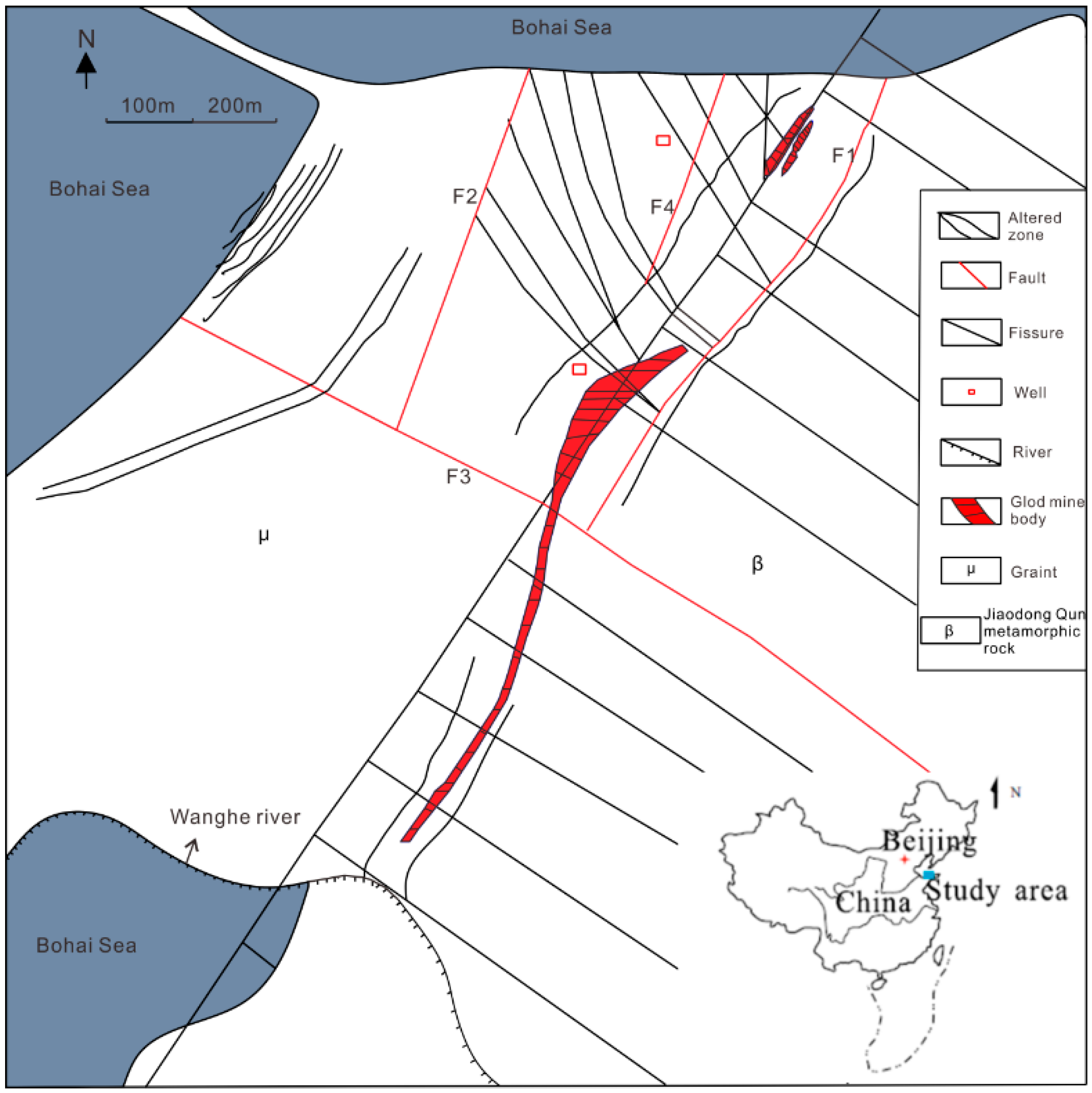
The Xishan gold mine is a part of the Sanshandao gold mine and is located in Laizhou Bay, Laizhou city, Shandong province, China. Three sides of the mining area are boarded by the Bohai Sea. In the southeast, it is connected to the land. There are three low connected hills southeast of the mining area. The highest elevation of the hills is 67.14 m. Except for three hills, the terrain is low, and the altitude generally ranges from 1 to 6 m and is covered by Quaternary sediment. The elevation of the south side of the mining area is 2–3.5 m, and the highest point is higher than the highest tide surface of the Bohai Sea, and the surface of the Bohai Sea is less than 1 m. Most of the mining areas are located below the intertidal zone and the seawater, and the ore beds do not have natural drainage.
The mining area belongs to the continental semi-humid climate of the temperate monsoon region and has four distinct seasons. Because of its proximity to the ocean, the area has both ocean and inland climate characteristics. The annual average temperature is 12.5 °C, and the precipitation is 612.1 mm. According to the differences in the lithology, Quaternary sediment can be divided into four units from top to bottom: (1) the first aquifer, which consists of medium and coarse sand. Its thickness ranges from 3.5 to 17.29 m, and the average thickness is 9.93 m. It contains groundwater in unconsolidated sediments, with the hydraulic conductivity ranging from 5.35 to 15.27 m/day. Additionally, its main renewable groundwater resources are atmospheric precipitation and seawater recharge. The total dissolved solids content varies considerably, with a minimum value of 0.21 g/L and a maximum value of 25.95 g/L; (2) the first aquiclude is located below the first aquifer. Its burry depth ranges from 5.5 to 9.0 m, and its thickness does not change obviously, with a general thickness of about 7 or 8 m; (3) the second aquifer gradually increases in thickness from north to south. Its average thickness is 3–4 m and has a maximum thickness of 11.9 m. It is a confined aquifer that can receive the recharge of the first aquifer and the seawater and is composed of medium sand, coarse sand, and gravel; (4) the second aquiclude is located above the weathered crust. Its thickness is 3–5 m and mainly comprises red clay, which makes it a good water barrier. There are three main water-controlling fractures, which have been named F1, F2, and F3, in the mining area (Figure 1). The maximum principle is horizontal, oriented NW–SE, and is perpendicular to the strike of F1.
The F1 fault is the ore-controlling structure of the mining area. The ore body is distributed in the footwall of the fault, which is inclined to the southeast and has a dip angle of 40°. There is a 50–100-mm-thick black gouge, which makes F1 an aquiclude [27].
The F2 fault is located west of F1 and is smaller than F1. F2 starts at the F3 fault and ends at the Bohai Sea; its strike is 280° and its dip is 85° [28]. F2 has the characteristics of a torsion fault, in which its hang wall moves northward, and the foot wall moves in the opposite direction. It is significantly different in terms of the fractures that have developed on both sides of F2. On the west side, the NE fracture is clearly developed, and a NW fracture is rare. On the east side, there is mainly a NW fracture. According to the results of geophysical exploration data, F2 has evident low-resistance characteristics, indicating that it is highly permeable.
The F3 fault is a regional fault that traverses the entire mining area—the Sanyuan–Chenjia fracture. The overall strike is 300–310°, which dips to the northwest with a dip angle of nearly 90°. It stretches northwest to the sea and southeast to the continent. The main fracture plane of F3 is located on the south side and is filled with gouge and fault breccia. The south side of the rock mass has perfect integrity and mainly develops NW–SE joints. According to current mining exploration, the depth is greater than 850 m, and the width of the fracture zone is approximately 15–35 m. At the ground surface, the broken belt is narrow, and the width increases as the depth increases. F3 is a tensile fracture, and there is no cement. It is a main groundwater pathway and has perfect hydraulic conductivity.
2.2. Water Sampling and Analysis
In the −375 m sublevel (Figure 2) of the Xishan gold mine, the water outlet sites were numbered. Two 600 mL bottles of water samples were collected from each water outlet site from 2009 to 2015 (Figure 3). Before the analysis, to ensure the quality of the water samples, the water samples were placed in 600 mL plastic bottles, sealed, and stored in a refrigerator at 4 °C.
The parameters of nine variables, including K+, Na−, Ca2+, Mg2+, Cl−, SO42−, HCO3−, pH, electrical conductivity (EC), and total dissolved solid (TDS), were measured at the Institute of Geology, China Earthquake Administration (Table 1). All water samples were measured by a DIONEX-500 ion chromatograph using EETROHMTM to test the CHO3− content in the water samples. The detection limits of cations and anions were 0.05 and 0.1 mg/L, respectively. The analysis accuracies of cations, anions, pH, EC, and TDS were 0.01 mg/L, 0.1 mg/L, 0.01, 0.1 μs/cm, and 0.01 mg/L, respectively. The test standards of cations, anions, and alkalinity were based on DZ/T0064.28-1993, DZ/Too64.51-1993, and DZ/T0064.29-1993, respectively [29]. The unit for the ions and the TDS concentrations was mg/L, the unit of EC was μs/cm, and the pH values were standard values. Another 600 mL bottle of the water sample was used for environmental isotope analysis (δ18O and δ2H). The analysis was conducted in the Laboratory for Stable Isotope Geochemistry, Institute of Geology and Geophysics (Beijing, China). An MT-253 mass spectrometer was used for isotope analysis with an analytical precision defined by two-sigma uncertainties of 0.2% for δ18O and 2% for δ2H. The values were all expressed in ‰. The value was according to the standard mean ocean water (SMOW; Appendix A, Table A1). The majority of chemistry data were primarily obtained between 375-1 and 375-9. Because the seasonal rainfall and fissure water decreased and dried out, some water samples of some water outlet sites were collected a few times. For example, the water sample of 375-2 was only obtained once in August 2009, and after 2009, 375-2 dried up. With the exploitation of the −375 m sublevel, the subway stretched forward gradually. Site 375-9 was added in 2012, thus there were only two water samples from this site.
2.3. Factor Analysis
Factor analysis is the generalization of PCA. It applies the dimension reduction theory of PCA to the internal structure of the correlation matrix of original variables. Factor analysis is a multivariate statistical analysis method used to reduce variables with related relationships into a few comprehensive factors. According to relevance, factor analysis divides variables into a few significant different groups, with a higher relevance in the same group and a lower relevance in a different group. The variables of each group are represented by a common structure (a common factor). The seven main ions accounted for 99% of the TDS, and EC is directly related to the amount of anions and cations. This finding can be interpreted as all the ions having some relevance (Table 2). Additionally, a statistical description of concentrations of the seven main ions is shown in Table 3. Combining variance and Pearson correlation can explain the dynamic evolution of groundwater solutes. From Table 3, the values of variance were sorted from large to small: Cl− > Na+ > Ca2+ > SO42−> Mg2+ > CHO3− > K+. The Cl− concentration had the most variance. Cl− is considered a conservative ion, thus the variance caused by the water-rock reaction in the groundwater mixing was negligible. Cl−, which had the most variance, had a good positive correlation with Na+ and Ca2+, with correlation coefficients of 0.956 and 0.842, respectively. This may have been due to inhomogeneous distributions of Cl−-bearing minerals and the different recharge of seawater and brine water. Ca2+ had a similar mean concentration as Mg2+. However, Ca2+ exhibited more variance than Mg2+. Ca2+ had a positive correlation with Cl− and a negative correlation with Mg2+ and CHO3−. In the mining area, beresite and lamprophyre, which contain a large amount of SO42−, were widely distributed. Calcite and dolomite were randomly distributed in fractures. These factors may have resulted in the larger variance value of Ca2+. The increased flow rate of the groundwater resulting from mining operations and CO2 fugacity in fractures could also increase the variance. The concentration of Mg2+ was correlated with Cl− and Na+, with correlation coefficients of −0.555 and −0.496, respectively. This might have been due to the rate and the amount of Quaternary water recharge containing Mg2+ being much greater than those of seawater.
In most geological studies, the relative magnitudes of variables are critical. Therefore, we attempted to conduct some work on the raw data. In cases where we had to standardize the data, we noted that a seemingly important property may have had a significant impact on the analysis. Standardization tends to inflate variables that display small variance and decrease the influence of variables with large variance [30]. The hydrochemical variables of the 31 water samples studied had different dimensions, and different dimensions caused large differences in the dispersion of each value of the variables. At that time, the total variance was controlled by the variables with large variance. To eliminate the effect due to different dimensions, we used a data normalization method to process the data and then performed a component analysis. In SPSS 25 software (IBM, Armonk, US), the data used for factor analysis and PCA were standardized. The Kaiser-Meyer-Olkin value was 0.585, and the Sig. value of Bartlett’s Sphericity was 0.00, which was less than 0.05. This demonstrated that all the samples were suitable for PCA or cluster analysis. A cluster analysis of the water chemistry data without treatment would lead to the repeated use of variable data, causing the geological information represented by the weighted water data to be used, resulting in distortion of the calculated cluster results. As such, factor analysis was used for processing the data, translating the related variables into orthogonal rotation factors, and the orthogonal rotation factors could then be used as new variables for the cluster analysis. Using SPSS 25 software to analyze the data, the original factor, the eigenvalues, and the total variance explained 10 of the variables (Table 4).
A cumulative variance contribution rate of 90% was considered to be a good explanation for hydrochemical information reflected in the data [31,32,33]. Therefore, extracting four original factors was reasonable. These four original factors accounted for 91.79% of the total variance. The purpose of establishing the factor analysis model was not only to identify the main factors but also to determine a clear meaning represented by the main factors to conduct a deeper analysis of the variables. Factor rotation can make the distinction between common factors more noticeable under the condition that the contribution rate of the common factors to the variable remains unchanged (Table 5).
2.4. Clustering Analysis
Clustering analysis is the main branch of multivariate statistical methods. Its primary purpose is to cluster water samples according to the properties of the variables. According to the Euclidean distance, clustering analysis divides water samples into a few groups, in which water samples in the same group have the most similar characteristics. The results of clustering analysis show that samples in the same group have the same properties, and vice versa. The most commonly used clustering method is hierarchical clustering analysis, which can identify the initial relationship between any sample and all the water sample data and visually demonstrate the relationship with a dendrogram of the clustering analysis. In this paper, the normalization matrix of the original data was multiplied by the component score coefficient matrix to obtain the factor score matrix, and the factor scores were then used as clustering variables. In MATLAB, the factor score matrix was obtained (Table 6). The factor scores matrix of the water sample variables was used to perform the clustering analysis. The clustering groups were connected by the Ward method, and the similarity of the factor scores was demonstrated by Euclidean distances. Euclidean distance is often used to describe the similarity of water samples and can express the difference in a sample’s value. Euclidean distance can be measured by the following equation [34]:
where i and k are two different water samples, j is the mode of the variables, and v is the value of the variables. The smaller the Euclidean distance D is, the more similar the water samples are. The D value quantitatively shows the degree of affinity between water samples.
2.5. Discriminant Analysis
Using some special principle rules—a dichotomy—discriminant analysis usually divides cases into a few groups. Correspondingly, the water samples that belong to the same group share common properties. Most importantly, discriminant analysis could establish discriminant functions of only the original data of two or more variables, thus we could determine which group the water samples belonged to. In discriminant analysis, not as many variables are possible, but the method should select the main variables to discriminate, because each variable has a special role. Some play a major role, and some play a minor role. Putting the variables that play minor roles into the discriminant function not only increases the number of calculations but also causes interference, which influences the discrimination effect. The stepwise discriminant analysis method is mainly based on the importance of each variable in the discriminant function for selecting the best variables [35]. Stepwise discriminant analysis gradually introduces the “most important” variable into the discriminant function and tests some of the variables that are introduced first. If the discriminant ability with the incoming new variables becomes insignificant, they are removed until no new other variables enter and no old variables are removed. We used the remaining water samples to establish the Bayes linear discriminant function. Among all the variables that we selected, pH, EC, and TDS were the most direct expressions of the seven common ions in the water samples, and those variables had a high degree of correlation.
The mode was established using SPSS 25 software; stepwise discriminant analysis of the data collected from the selected water samples was performed, and the Bayes linear discriminant function was obtained as follows:
where M1 is the mode of the water samples from 375-5 and 375-6, M2 is the mode of the other water samples, and V() and V() are the corresponding ion mass concentrations.
3. Results of Multivariate Statistical Analysis
Not all variables are isolated in the water of the laneways. The greater the correlation between ions is, the higher the degree of coincidence geological information is. Using SPSS 25 software to determine the correlations of the 10 variables, the results demonstrated that Na+ had a strong positive correlation with Cl−; Ca2+ had a strong negative correlation with Mg2+ and CHO3−, instead of a positive correlation with TDS; Mg2+ had a strong positive correlation with CHO3−; Cl− had a strong positive correlation with Ca2+, TDS, EC, and TDS (Table 2).
Using the maximum variance method to rotate the factor load, after 13 iterations, the result converged. The variance of the variables became more significantly different, and the contribution rate of the variables for a special factor was more easily obtained (Table 5). Fa1 had a large factor load in Na+, Ca2+, Mg2+, Cl−, CHO3−, and TDS. Fa2 had a large factor load in Na+, pH, and EC. Fa3 had a large factor load in K+, and Fa4 had a large factor load in SO42−. The factor load matrix is the basis for calculating the component score coefficient matrix. The factor load matrix’s component score coefficient matrix is shown in Table 7.
According to the results of the clustering analysis (Table 8), three water samples from 375-6-3, 375-7-1, and 375-8-1, which were defined as incorrect, were removed, and 375-1-2 and 375-4-4 were selected as the testing water samples (Table 9). We analyzed 31 water samples with SPSS 25 with the clustering method, and the results are presented in Figure 4. From the dendrogram of the hierarchical clustering analysis, we observed that, between the 1740 line and the 2740 line at the −375 m sublevel, the style of the water sample site was clearly divided into two statistically significant clusters at (Dlink/Dmax) × 100 < 60 [32]. The 375-1, 375-2, 375-3, 375-4, 375-7, 375-8, and 375-9 samples belonged to the first mode (M1), and the 375-5 and the 375-6 samples belonged to another mode (M2). The locations of 375-5 and 375-6 were very close (Figure 2), and their close distance supported their similarity. Initially, due to tunnel excavation, a large amount of artificial drainage occurred, and groundwater flow accelerated, which removed much of the brine. Seawater and Quaternary water, which have a high hydraulic gradient, infiltrated the −375 m sublevel through bedrock fractures. Simultaneously, the F3 fault and the NW-oriented fractures opened due to mining-induced rock movement and stress redistribution [7,36]. M2 water samples that were affected by the F3 fault mainly received the vertical recharge of Quaternary water and partially received the lateral recharge of seawater. However, M1 water samples, which were affected by NW-oriented fractures and were obtained far away from the F3 fault, mainly received the lateral recharge of seawater and partially received the vertical recharge of Quaternary water. Therefore, according to the hydrological conditions and the results of cluster analysis, the water samples in the −375 m sublevel could be divided into two typical modes (M1 and M2).
According to the Bayes posterior probability principle, the corresponding ion mass concentration was brought into the Bayes linear discriminant function. The function with a larger value determined the mode. The corresponding ion mass concentrations of 26 water samples and two test water samples were brought into the above two Bayes linear discriminant functions, and the resulting data are provided in Table 8. The cross-comparison between the results (Figure 4) of hierarchical clustering analysis and the results (Table 8) of stepwise discriminant analysis showed that the Bayes linear function established by the stepwise discriminant analysis method achieved 100% accuracy in identifying the water sources.
4. Discussion
Groundwater dynamics are complex, and this complexity is enhanced by the heterogeneity of the rock mass and the mining operations. The apertures of faults and fractures can open or close due to mining activities. Frequently, due to the release of underground stress, the fault is activated or the fractures are expanded, which can then intensify the flow rate of groundwater. For coastal mining operations, research on the roadway fracture network is critical.
The combined multivariate statistical methods were used to successfully identify groundwater sources and assess groundwater dynamics. According to the factor analysis results, the factor scores were plotted in Figure 5, which shows that the groundwater was divided into two types. From the location of water sites (Figure 2), M1 was close to the F3 fault, and M2 had a relatively large Euclidean distance compared to M1.
In this studied area, the recharge sources of groundwater are mainly freshwater, Quaternary water, and seawater. In the process of groundwater mixing, ion exchanges and hydrochemical reactions occur. However, using stable isotopes (δ18O and δ2H) to identify groundwater is reliable, because they are considered conservative tracers. The values of δ18O and δ2H (Appendix A Table A1) are plotted in Figure 6, which also includes the global meteoric water line (GMWL) and the local meteoric water line (LMWL). The δ18O and the δ2H values from −375 m sublevel water samples ranged from −24.546‰ to −6.478‰ and from −3.328 to −1.215, respectively. The δ18O and the δ2H values of freshwater were −7.543‰ and −53.44‰, respectively. The δ18O and the δ2H values of the Quaternary water were −3.585 ‰ and −32.03‰ respectively, whereas the seawater had the greatest values (0.036‰ and −5.405‰, respectively) of δ18O and δ2H. All values except those for the site 375-6-4 were plotted in a polygon defined by freshwater, Quaternary water, seawater, and LMWL. This demonstrated that all water samples were mixes of these three types of water. M1 was nearing the Quaternary water. This demonstrated that M1 samples were mainly composed of Quaternary water. M2 was located between seawater and Quaternary water. The mixing of seawater and Quaternary water explained the M2 samples. The F3 fault and the NW–NE fractures had a significant effect on groundwater sources. A field investigation revealed that the F3 fault, whose width of the fracture zone was approximately 15–35 m, was a deep fault, and in the −375 m sublevel, there were 471 fractures with three prior attitudes: 38° < 89°, 16° < 15°, and 120° < 83°. Above the −600 m sublevel, Quaternary water and seawater were dominant sources, and F3 and the NW-oriented fractures were the main channels for these sources for deeper parts of tunnels [7,36]. M1 water samples were recharged by Quaternary water through the F3 fault in the vertical direction, and M2 water samples were partly recharged by Quaternary water in the vertical direction through the F3 fault and mostly by seawater in the lateral direction through NW−NE fractures.
The combination of multivariate statistical analysis methods enables deriving a Bayes linear function that quantifies the type of water source. The method proposed in this paper is different from most presented in other research. We focused on types of water samples and rapidly and economically determined the specific type of water to which the samples belonged. However, some research [14,15,16,20,37] has been dedicated to studying the specific proportion of end-members of mixed water samples. Because of existing hydrochemical reactions, the end-members were uncertain. Although the specific proportion of end-members was known, it was not possible to determine which type of water belonged to which sample. Other studies [38,39,40] used PCA and clustering analysis to determine the water sources. This multivariate statistical analysis could also identify water source types, but it did not have a self-test feature and could not produce simple and direct functions. From the above discussion, we found that groundwater of the −375 m sublevel mainly consisted of seawater and Quaternary water. The F3 fault was the main vertical recharge channel of Quaternary water, and NW-oriented fractures were the main lateral recharge channel of seawater. The ratio of these two water sources is considerably different at different water sites, depending on the apertures of fractures caused by mining-induced stress redistribution. We speculate that lateral seawater recharge is the main source of mine water inrush, and the F3 fault is a potential channel of water inrush. Therefore, the water chemistry and the flow monitoring of M1 water samples are the focus of our attention.
5. Conclusions
In the study area, because of mining operations, the Quaternary aquifer was broken, and groundwater flow accelerated. This led to a recharge of seawater and freshwater becoming the dominant water source, with a small amount of vertical recharge occasionally occurring. The depth of recharge had already reached −510 m at the time of the study. In particular, the proportion of freshwater at most sites above −375 m exceeded 40%. [36]. It is possible to study the likelihood of intrusion and identify the water source type. The multivariate statistical analysis described here is useful for identifying the sources’ types of mine groundwater.
- (1)
- According to the hydrochemical information of the water samples from Xishan gold mine, the hydrochemical data were preprocessed, and the water samples were divided into M1 and M2 by factor analysis combined with principle component analysis. Among the 31 water samples, three were discriminated incorrectly, and the correct rate of discrimination was 90.3%.
- (2)
- Stepwise discriminant analysis and factor analysis were combined to process the data of seven conventional ions. The Bayes linear discriminant function and function values from the 1740 exploration line to 2740 exploration line in the −375 m sublevel were obtained. The Bayes linear function discriminant results were completely consistent with the results of the factor analysis method, and the two selected discriminant water samples also agreed. The consistency of the discriminant results showed that the factor analysis method and the stepwise analysis method were mutually verified.
- (3)
- A multivariate statistical method was combined to obtain a quantitative Bayes linear discriminant function, which was applied to recognize the source type in the mining area. It was only necessary to know the ion concentration of the corresponding variable, and the water sample type could be determined by substituting the value of the corresponding variable. This method is accurate, fast, and economical.
The method introduced in this paper could not identify fuzzy water samples that were close in terms of distance or extremely similar in water chemistry and could not provide specific measurements and prevention of mine water inrush. However, the method, which is fast and economical, could accurately identify the type of water sample in the study area. More importantly, this method has barely been studied and is universal for almost all water-bearing mines. The method was applied to other water-containing roadways of mines to identify groundwater sources, and then, according to the hydrogeological conditions, Bayes functions were finally obtained, which may serve as a scientific basis to solve mine water inrush problems.
Author Contributions
Conceptualization, G.L. (Guowei Liu); Formal analysis, J.G.; Funding acquisition, F.M.; Investigation, G.L. (Guowei Liu), G.L. (Gang Liu) and J.C.; Supervision, F.M. and H.Z.; Validation, G.L. (Gang Liu); Writing—original draft, G.L. (Guowei Liu); Writing—review & editing, G.L. (Guowei Liu).
Funding
This work has been conducted in the framework of the National Key Research Projects of China (2016YFC0402802) and financially supported by the National Science Foundation of China (Grant nos. 41772341).
Conflicts of Interest
The authors declare no conflict of interest.
Appendix A

Table A1.
δ18O and δD The values of water samples from 2009 to 2015. Sea water, Quaternary water and freshwater were collected in 2009.
Table A1.
δ18O and δD The values of water samples from 2009 to 2015. Sea water, Quaternary water and freshwater were collected in 2009.
| ID | δD | δ18O (‰) |
|---|---|---|
| 375-1-1 | −16.907 | −1.458 |
| 375-1-2 | −11.247 | −2.304 |
| 375-1-3 | −17.518 | −1.895 |
| 375-1-4 | −23.531 | −2.076 |
| 375-1-5 | −6.478 | −2.258 |
| 375-2-1 | −15.49 | −1.35 |
| 375-3-1 | −13.573 | −1.215 |
| 375-3-2 | −8.703 | −1.916 |
| 375-3-3 | −21.602 | −2.404 |
| 375-4-1 | −15.387 | −1.33 |
| 375-4-2 | −14.047 | −1.983 |
| 375-4-3 | −14.633 | −1.807 |
| 375-4-4 | −23.488 | −2.207 |
| 375-4-5 | −17.478 | −1.799 |
| 375-5-1 | −24.546 | −2.694 |
| 375-5-2 | −18.458 | −2.583 |
| 375-5-3 | −24.136 | −2.83 |
| 375-5-4 | −29.88 | −3.328 |
| 375-5-5 | −11.362 | −2.88 |
| 375-6-1 | −18.47 | −2.129 |
| 375-6-2 | −17.286 | −2.525 |
| 375-6-3 | −12.475 | −1.515 |
| 375-7-1 | −21.256 | −2.234 |
| 375-7-2 | −13.0051 | −1.97206 |
| 375-7-3 | −11.4324 | −1.28895 |
| 375-8-1 | −12.7097 | −2.11231 |
| 375-8-2 | −18.502 | −1.571 |
| 375-8-3 | −12.581 | −2.135 |
| 375-8-4 | −14.1866 | −1.49238 |
| 375-9-1 | −10.337 | −1.20527 |
| 375-9-2 | −13.4648 | −1.70191 |
| Quaternary water | −32.03 | −3.585 |
| Freshwater | −53.44 | −7.543 |
| Sea water | −5.18 | −0.181 |
References
- Wu, J.; Xu, S.; Zhou, R.; Qin, Y. Scenario analysis of mine water inrush hazard using Bayesian networks. Saf. Sci. 2016, 89, 231–239. [Google Scholar] [CrossRef]
- Epstein, R.; Goic, M.; Weintraub, A.; Catalán, J.; Santibáñez, P.; Urrutia, R.; Cancino, R.; Gaete, S.; Aguayo, A.; Caro, F. Optimizing Long-Term Production Plans in Underground and Open-Pit Copper Mines. Oper. Res. 2012, 60, 4–17. [Google Scholar] [CrossRef]
- Unlu, T.; Akcin, H.; Yilmaz, O. An integrated approach for the prediction of subsidence for coal mining basins. Eng. Geol. 2013, 166, 186–203. [Google Scholar] [CrossRef]
- Meng, Z.; Li, G.; Xie, X. A geological assessment method of floor water inrush risk and its application. Eng. Geol. 2012, 143–144, 51–60. [Google Scholar] [CrossRef]
- Ma, D.; Rezania, M.; Yu, H.S.; Bai, H.B. Variations of hydraulic properties of granular sandstones during water inrush: Effect of small particle migration. Eng. Geol. 2017, 217, 61–70. [Google Scholar] [CrossRef] [Green Version]
- Bai, H.; Ma, D.; Chen, Z. Mechanical behavior of groundwater seepage in karst collapse pillars. Eng. Geol. 2013, 164, 101–106. [Google Scholar] [CrossRef]
- Gu, H.; Ma, F.; Guo, J.; Li, K.; Lu, R. Assessment of Water Sources and Mixing of Groundwater in a Coastal Mine: The Sanshandao Gold Mine, China. Mine Water Environ. 2017, 37, 351–365. [Google Scholar] [CrossRef]
- Janson, E.; Boyce, A.J.; Burnside, N.; Gzyl, G. Preliminary investigation on temperature, chemistry and isotopes of mine water pumped in Bytom geological basin (USCB Poland) as a potential geothermal energy source. Int. J. Coal Geol. 2016, 164, 104–114. [Google Scholar] [CrossRef]
- Wang, J.; Lu, C.; Sun, Q.; Xiao, W.; Cao, G.; Li, H.; Yan, L.; Zhang, B. Simulating the hydrologic cycle in coal mining subsidence areas with a distributed hydrologic model. Sci. Rep. 2017, 7, 39983. [Google Scholar] [CrossRef]
- Liu, Y.; An, S.; Xu, Z.; Fan, N.; Cui, J.; Wang, Z.; Liu, S.; Pan, J.; Lin, G. Spatio-temporal variation of stable isotopes of river waters, water source identification and water security in the Heishui Valley (China) during the dry-season. Hydrogeol. J. 2008, 16, 311–319. [Google Scholar] [CrossRef]
- Wang, J.; Zhao, J.; Lei, X.; Wang, H. New approach for point pollution source identification in rivers based on the backward probability method. Environ. Pollut. 2018, 241, 759–774. [Google Scholar] [CrossRef]
- Huang, P.; Chen, J. Recharge sources and hydrogeochemical evolution of groundwater in the coal-mining district of Jiaozuo, China. Hydrogeol. J. 2012, 20, 739–754. [Google Scholar] [CrossRef]
- Christophersen, N.; Hooper, R.P. Multivariate analysis of stream water chemical data: The use of principal components analysis for the end-member mixing problem. Water Resour. Res. 1992, 28, 99–107. [Google Scholar] [CrossRef]
- Doctor, D.H.; Alexander, E.C.; Petrič, M.; Kogovšek, J.; Urbanc, J.; Lojen, S.; Stichler, W. Quantification of karst aquifer discharge components during storm events through end-member mixing analysis using natural chemistry and stable isotopes as tracers. Hydrogeol. J. 2006, 14, 1171–1191. [Google Scholar] [CrossRef]
- Laaksoharju, M.; Skårman, C.; Skårman, E. Multivariate mixing and mass balance (M3) calculations, a new tool for decoding hydrogeochemical information. Appl. Geochem. 1999, 14, 861–871. [Google Scholar] [CrossRef]
- Carrera, J.; Vázquez-Suñé, E.; Castillo, O.; Sánchez-Vila, X. A methodology to compute mixing ratios with uncertain end-members. Water Resour. Res. 2004, 40, 12101–12112. [Google Scholar] [CrossRef]
- Güler, C.; Thyne, G.D. Delineation of hydrochemical facies distribution in a regional groundwater system by means of fuzzy c-means clustering. Water Resour. Res. 2004, 40, 12503–12515. [Google Scholar]
- Li, K.; Ma, F.; Zhang, H.; Li, W.; Lv, Y. Recharge resource identification and evolution Inflowing-water in a sea bed gold mine. J. Eng. Geol. 2017, 25, 180–189. (In Chinese) [Google Scholar]
- Chen, K.; Jiao, J.J.; Huang, J.; Huang, R. Multivariate statistical evaluation of trace elements in groundwater in a coastal area in Shenzhen, China. Environ. Pollut. 2007, 147, 771–780. [Google Scholar] [CrossRef]
- Long, A.J.; Valder, J.F. Multivariate analyses with end-member mixing to characterize groundwater flow: Wind Cave and associated aquifers. J. Hydrol. 2011, 409, 315–327. [Google Scholar] [CrossRef]
- Hao, Z.; Duoxi, Y.; Haifeng, L.; Ningning, Z.; Liang, X. Application of principal component analysis and Bayes discrimination approach in water source identification. Coal Geol. Explor. 2017, 16. [Google Scholar]
- Raiber, M.; White, P.A.; Daughney, C.J.; Tschritter, C.; Davidson, P.; Bainbridge, S.E. Three-dimensional geological modelling and multivariate statistical analysis of water chemistry data to analyse and visualise aquifer structure and groundwater composition in the Wairau Plain, Marlborough District, New Zealand. J. Hydrol. 2012, 436, 13–34. [Google Scholar] [CrossRef]
- Qian, J.; Wang, L.; Ma, L.; Lu, Y.; Zhao, W.; Zhang, Y. Multivariate statistical analysis of water chemistry in evaluating groundwater geochemical evolution and aquifer connectivity near a large coal mine, Anhui, China. Environ. Earth Sci. 2016, 75, 747. [Google Scholar] [CrossRef]
- Wang, Y.; Wang, P.; Bai, Y.; Tian, Z.; Li, J.; Shao, X.; Mustavich, L.F.; Li, B.L. Assessment of surface water quality via multivariate statistical techniques: A case study of the Songhua River Harbin region, China. J. Hydro-Environ. Res. 2013, 7, 30–40. [Google Scholar] [CrossRef]
- Granato, D.; Santos, J.S.; Escher, G.B.; Ferreira, B.L.; Maggio, R.M. Use of principal component analysis (PCA) and hierarchical cluster analysis (HCA) for multivariate association between bioactive compounds and functional properties in foods: A critical perspective. Trends Food Sci. Technol. 2018, 72, 83–90. [Google Scholar] [CrossRef]
- Williams, M.R.; Leydecker, A.; Brown, A.D.; Melack, J.M. Processes regulating the solute concentrations of snowmelt runoff in two subalpine catchments of the Sierra Nevada, California. Water Resour. Res. 2001, 37, 1993–2008. [Google Scholar] [CrossRef]
- Liu, C. The geological analysis and modelling of mining water flow-as an example of San Shan island gold mine. J. Eng. Geol. 1994, 25, 180–189. (In Chinese) [Google Scholar]
- GU, H. A Study of Water Sources and Flow Paths in a Coastal Gold Mine; Institute of Geology and Geophysics; Chinese Academy of Sciences: Beijing, China, 2018. [Google Scholar]
- Ma, F.; Zhao, H.; Guo, J. Investigating the characteristics of mine water in a subsea mine using groundwater geochemistry and stable isotopes. Environ. Earth Sci. 2015, 74, 6703–6715. [Google Scholar] [CrossRef]
- Davis, J.C. Statitics and Data Analysis in Geology, 2nd ed.; John Wiley & Sons, Inc.: Hoboken, NJ, USA, 2002; p. 536. [Google Scholar]
- Friston, K.J.; Frith, C.D.; Liddle, P.F.; Frackowiak, R.S.J. Functional Connectivity: The Principal-Component Analysis of Large (PET) Data Sets. J. Cereb. Blood Flow Metab. 1993, 13, 5–14. [Google Scholar] [CrossRef]
- Salifu, A.; Petrusevski, B.; Ghebremichael, K.; Buamah, R.; Amy, G. Multivariate statistical analysis for fluoride occurrence in groundwater in the Northern region of Ghana. J. Contam. Hydrol. 2012, 140, 34–44. [Google Scholar] [CrossRef]
- Shrestha, S.; Kazama, F. Assessment of surface water quality using multivariate statistical techniques: A case study of the Fuji river basin, Japan. Environ. Model. Softw. 2007, 22, 464–475. [Google Scholar] [CrossRef]
- Otto, M. Multivariate methods. In Analytical Chemistry; Kellner, R., Mermet, J.M., Otto, M., Widmer, H.M., Eds.; Wiley-VCH: Weinheim, Germany, 1998. [Google Scholar]
- Xiang, D.; Li, H.; Liu, X. Applied Multivariate Statistical Analysis; China University of Geosciences Press: Wuhan, China, 2005. (In Chinese) [Google Scholar]
- Gu, H.; Ma, F.; Guo, J.; Zhao, H.; Lu, R.; Liu, G. A spatial mixing model to assess groundwater dynamics affected by mining in a coastal fractured aquifer, China. Mine Water Environ. 2018, 37, 405–420. [Google Scholar] [CrossRef]
- Delsman, J.R.; Essink, G.H.O.; Beven, K.J.; Stuyfzand, P.J. Uncertainty estimation of end-member mixing using generalized likelihood uncertainty estimation (GLUE), applied in a lowland catchment. Water Resour. Res. 2013, 49, 4792–4806. [Google Scholar] [CrossRef] [Green Version]
- Cao, X.; Qian, J.; Sun, X. Hydrochemical classification and identification for groundwater system by using integral multivariate statistical models: A case study in Guqiao Mine. J. China Coal Soc. 2010, 35, 0141–0144. [Google Scholar]
- Liu, J.; Xue, X.; Shi, Y.; Yu, Q.; Li, L. Application of multivariate statistical analysis model to identification of water inrush source in coal mines. China Coal 2013, 39, 101–104. [Google Scholar] [CrossRef]
- Li, J.; Su, C.; Xie, X.; Wang, Y. Application of multivariate statistical analysis to research the environment of groundwater: A case study at Datong basin, Northern China. Geol. Sci. Technol. Inf. 2010, 29, 94–100. [Google Scholar]
Figure 1.
Sketch of the study area.

Figure 2.
Water sites of the −375 m sublevel.

Figure 3.
Field collection of water samples.

Figure 4.
Dendrogram of the hierarchical clustering analysis.

Figure 5.
Factor scores obtained by cluster analysis: (a) Fa1 vs. Fa2 and (b) Fa1 vs. Fa3. Fa1, Fa2, and Fa3 account for 83.5% of the total variance.
Figure 5.
Factor scores obtained by cluster analysis: (a) Fa1 vs. Fa2 and (b) Fa1 vs. Fa3. Fa1, Fa2, and Fa3 account for 83.5% of the total variance.

Figure 6.
Environmental isotopes δ18O vs. δ2H for all water samples from the −375 m sublevel from 2009 to 2015. Seawater, Quaternary water, and freshwater were collected in 2009.
Figure 6.
Environmental isotopes δ18O vs. δ2H for all water samples from the −375 m sublevel from 2009 to 2015. Seawater, Quaternary water, and freshwater were collected in 2009.

Table 1.
Statistics of the hydrochemical parameters of water samples from the −375 m sublevel from 2009 to 2015.
Table 1.
Statistics of the hydrochemical parameters of water samples from the −375 m sublevel from 2009 to 2015.
| Location | K+ | Na+ | Ca2+ | Mg2+ | Cl− | SO42− | HCO3− | pH | EC | TDS |
|---|---|---|---|---|---|---|---|---|---|---|
| (mg/L) | (mg/L) | (mg/L) | (mg/L) | (mg/L) | (mg/L) | (mg/L) | (μs/cm) | (mg/L) | ||
| 375-1-1 | 248.4 | 104,00 | 761.5 | 1287.9 | 19,852 | 2305.4 | 219.6 | 7.19 | 44,900 | 35,074.8 |
| 375-1-2 | 197 | 9750 | 801.6 | 1222.3 | 18,453.5 | 2334.3 | 233.7 | 7.74 | 39,600 | 32,995 |
| 375-1-3 | 205 | 10,031.2 | 849.7 | 1239.3 | 18,916.1 | 2497.6 | 244.6 | 7.07 | 42,300 | 33,991.5 |
| 375-1-4 | 190.2 | 9800 | 841.7 | 1215 | 19,224.5 | 624.4 | 250.7 | 7.31 | 42,100 | 32,147.5 |
| 375-1-5 | 179.7 | 9875 | 721.4 | 1166.4 | 18,402.1 | 2372.7 | 253.2 | 7.34 | 40,000 | 32,974.6 |
| 375-2-1 | 286 | 10,650 | 697.4 | 1312.2 | 19,852 | 2286.2 | 207.4 | 7.03 | 45,200 | 35,292.8 |
| 375-3-1 | 299.2 | 9445 | 537.1 | 1132.4 | 17,583.2 | 2017.3 | 219.6 | 7.36 | 40,800 | 31,233.8 |
| 375-3-2 | 241 | 8900 | 681.4 | 1040 | 16,705.8 | 2190.2 | 233.7 | 7.56 | 37,000 | 29,992.1 |
| 375-3-3 | 275.8 | 9200 | 753.5 | 1069.2 | 17,579.7 | 2286.2 | 273.3 | 7.45 | 39,800 | 31,437.9 |
| 375-4-1 | 316.8 | 9825 | 641.3 | 1044.9 | 17,583.2 | 2017.3 | 201.3 | 7.49 | 41,100 | 31,629.8 |
| 375-4-2 | 258 | 8900 | 921.8 | 945.3 | 17,014.2 | 2295.8 | 181.2 | 7.46 | 37,200 | 30,516.3 |
| 375-4-3 | 282.5 | 9725 | 1122.2 | 1001.2 | 18,607.7 | 2516.8 | 170.8 | 7.11 | 41,800 | 33,433.8 |
| 375-4-4 | 285.5 | 9900 | 1314.6 | 831.1 | 18,710.5 | 2401.5 | 168.4 | 7.32 | 40,800 | 33,614.5 |
| 375-4-5 | 285.1 | 10,000 | 1154.3 | 916.1 | 18,874.3 | 2401.5 | 170.8 | 7.03 | 40,900 | 33,821.3 |
| 375-5-1 | 260 | 12,050 | 1146.3 | 1020.6 | 21,979 | 2459.1 | 119.6 | 7.29 | 50,400 | 39,052.7 |
| 375-5-2 | 208 | 10,886.2 | 1523 | 972 | 20,818 | 2545.6 | 114.1 | 7.41 | 42,500 | 37,081.6 |
| 375-5-3 | 195 | 10,900 | 1595.2 | 957.4 | 19,738.6 | 2708.9 | 108 | 7.05 | 45,800 | 36,216.5 |
| 375-5-4 | 226.5 | 11,250 | 1643.3 | 823.8 | 21,280.6 | 2603.2 | 85.4 | 7.32 | 44,700 | 37,916.2 |
| 375-5-5 | 252.5 | 11,500 | 1971.9 | 517.6 | 21,471.7 | 2353.5 | 81.8 | 7.03 | 44,700 | 38,156.3 |
| 375-6-1 | 337.5 | 11,450 | 2084.2 | 777.6 | 22,156.3 | 2497.6 | 107.4 | 7.02 | 49,700 | 39,411.6 |
| 375-6-2 | 262 | 11,819 | 2276.5 | 726.6 | 22,411.5 | 2488 | 108 | 7.06 | 44,400 | 40,117.1 |
| 375-6-3 | 257.8 | 9062.5 | 505 | 1142.1 | 17,560.5 | 2315 | 236.1 | 7.64 | 34,500 | 31,080.1 |
| 375-7-1 | 305 | 10,700 | 1723.4 | 923.4 | 21,270 | 2363.1 | 134.2 | 7.17 | 48,100 | 37,424.9 |
| 375-7-2 | 251 | 9562.5 | 521 | 1154.3 | 17,642.4 | 2353.5 | 225.7 | 7.16 | 39,300 | 31,716.5 |
| 375-7-3 | 265.6 | 9187.5 | 481 | 1161.5 | 17,731.7 | 2238.2 | 230 | 7.66 | 34,400 | 31,296.2 |
| 375-8-1 | 290.4 | 10,350 | 1026 | 1078.9 | 18,965.7 | 1729.1 | 158.6 | 7.3 | 44,100 | 33,598.7 |
| 375-8-2 | 294 | 10,937.5 | 2312.6 | 626.9 | 21,794.7 | 2257.4 | 102.5 | 7.66 | 43,900 | 38,344.7 |
| 375-8-3 | 198.1 | 10,438 | 721.4 | 1287.9 | 19,597.1 | 2401.5 | 233.7 | 7.22 | 43,000 | 34,884 |
| 375-8-4 | 281.3 | 9062.5 | 521 | 1154.3 | 17,389.3 | 2353.5 | 230 | 7.54 | 35,000 | 30,992.4 |
| 375-9-1 | 205 | 10,375 | 681.4 | 1268.5 | 18,919 | 2449.5 | 256.2 | 7.63 | 42,500 | 34,154.6 |
| 375-9-2 | 262.5 | 9250 | 521 | 1154.3 | 17,731.7 | 2343.9 | 222.7 | 7.57 | 34,900 | 31,486.7 |
EC, electrical conductivity; TDS, total dissolved solutions.
Table 2.
Pearson correlation matrix of variables.
| K+ | Na+ | Ca2+ | Mg2+ | Cl− | SO42− | CHO3− | pH | EC | TDS | |
|---|---|---|---|---|---|---|---|---|---|---|
| K+ | 1.000 | 0.010 | 0.194 | −0.366 | 0.065 | 0.037 | −0.270 | −0.105 | 0.112 | 0.065 |
| Na+ | 1.000 | 0.763 | −0.496 | 0.956 | 0.260 | −0.766 | −0.522 | 0.878 | 0.969 | |
| Ca2+ | 1.000 | −0.860 | 0.842 | 0.254 | −0.880 | −0.398 | 0.640 | 0.854 | ||
| Mg2+ | 1.000 | −0.555 | −0.237 | 0.829 | 0.235 | −0.334 | −0.576 | |||
| Cl− | 1.000 | 0.209 | −0.777 | −0.470 | 0.835 | 0.987 | ||||
| SO42− | 1.000 | −0.328 | −0.152 | 0.117 | 0.345 | |||||
| CHO3− | 1.000 | 0.404 | −0.621 | −0.805 | ||||||
| pH | 1.000 | −0.624 | −0.495 | |||||||
| EC | 1.000 | 0.839 | ||||||||
| TDS | 1.000 |
Note: Significant loadings (>0.7) are in bold.
Table 3.
Statistical descriptions of all variables.
| Variable | Number | Minimum | Maximum | Mean | Variance |
|---|---|---|---|---|---|
| K+ | 31 | 179.70 | 337.50 | 254.92 | 1704.81 |
| Na+ | 31 | 8900.00 | 12,050.00 | 10,167.16 | 777,901.29 |
| Ca2+ | 31 | 481.00 | 2312.60 | 1066.25 | 308,912.05 |
| Mg2+ | 31 | 517.60 | 1312.20 | 1037.77 | 39,872.52 |
| Cl− | 31 | 16,705.80 | 22,411.50 | 19,219.89 | 2,828,300.73 |
| SO42− | 31 | 624.40 | 2708.90 | 2290.57 | 129,613.43 |
| CHO3− | 31 | 81.80 | 273.30 | 186.53 | 3462.04 |
| pH | 31 | 7.02 | 7.74 | 7.33 | 0.05 |
| EC | 31 | 34,400.00 | 50,400.00 | 41,787.10 | 17,233,161.29 |
| TDS | 31 | 29,992.10 | 40,117.10 | 34,228.60 | 8,749,166.58 |
Table 4.
Total variance explained.
| Principle Component | Eigenvalues | ||
|---|---|---|---|
| Value | Variance (%) | Cumulative Variance (%) | |
| 1 | 6.048 | 60.476 | 60.476 |
| 2 | 1.331 | 13.311 | 73.787 |
| 3 | 0.972 | 9.715 | 83.502 |
| 4 | 0.829 | 8.290 | 91.792 |
| 5 | 0.500 | 5.003 | 96.794 |
| 6 | 0.137 | 1.370 | 98.164 |
| 7 | 0.110 | 1.099 | 99.263 |
| 8 | 0.059 | 0.591 | 99.854 |
| 9 | 0.015 | 0.146 | 100.000 |
| 10 | 0.000002 | 0.000018 | 100.000 |
Table 5.
Factor load matrix.
| Factor Loadings | Rotated Factor Loadings | ||||||||
|---|---|---|---|---|---|---|---|---|---|
| Fa1 | Fa2 | Fa3 | Fa4 | Fa11 | Fa21 | Fa31 | Fa41 | HI2 | |
| K+ | 0.195 | −0.712 | −0.451 | 0.393 | 0.136 | 0.055 | −0.938 | −0.011 | 0.90 |
| Na+ | 0.933 | 0.272 | 0.014 | −0.049 | 0.695 | 0.652 | 0.178 | 0.083 | 0.95 |
| Ca2+ | 0.918 | −0.212 | 0.030 | −0.213 | 0.915 | 0.282 | −0.100 | 0.086 | 0.93 |
| Mg2+ | −0.722 | 0.575 | −0.032 | 0.213 | −0.869 | 0.033 | 0.359 | −0.117 | 0.90 |
| Cl− | 0.945 | 0.185 | −0.024 | −0.136 | 0.770 | 0.578 | 0.135 | 0.022 | 0.95 |
| SO42− | 0.330 | −0.166 | 0.794 | 0.473 | 0.170 | 0.076 | 0.006 | 0.977 | 0.99 |
| CHO3− | −0.900 | 0.273 | −0.059 | 0.096 | −0.865 | −0.289 | 0.185 | −0.179 | 0.90 |
| pH | −0.575 | −0.297 | 0.264 | −0.557 | −0.071 | −0.861 | 0.195 | −0.120 | 0.80 |
| EC | 0.837 | 0.353 | −0.235 | 0.130 | 0.478 | 0.815 | 0.044 | −0.052 | 0.90 |
| TDS | 0.966 | 0.161 | 0.084 | -0.053 | 0.765 | 0.583 | 0.127 | 0.161 | 0.97 |
Note: Significant loadings (>0.6) are in bold.
Table 6.
Factor scores of the water samples.
| Water Samples | Factor Scores | |||
|---|---|---|---|---|
| Fa1 | Fa2 | Fa3 | Fa4 | |
| 375-1-1 | 0.145 | 1.681 | −0.299 | 0.707 |
| 375-1-2 | −4.660 | 0.781 | 1.220 | −1.139 |
| 375-1-3 | −1.536 | 1.969 | 0.566 | 0.858 |
| 375-1-4 | −4.660 | 2.575 | −3.173 | −2.340 |
| 375-1-5 | −3.639 | 1.595 | 0.991 | −0.270 |
| 375-2-1 | 1.180 | 1.388 | −0.940 | 1.441 |
| 375-3-1 | −4.223 | −0.812 | −1.128 | 0.426 |
| 375-3-2 | −6.907 | −1.024 | 0.311 | −0.483 |
| 375-3-3 | −5.205 | −0.758 | −0.156 | 0.309 |
| 375-4-1 | −3.236 | −1.471 | −1.133 | 0.118 |
| 375-4-2 | −4.830 | −1.697 | 0.311 | −0.176 |
| 375-4-3 | 0.083 | −0.688 | −0.063 | 1.154 |
| 375-4-4 | 0.297 | −1.496 | −0.008 | 0.251 |
| 375-4-5 | 0.903 | −0.763 | −0.363 | 1.059 |
| 375-5-1 | 8.111 | 1.430 | −0.023 | 0.119 |
| 375-5-2 | 3.954 | 0.656 | 1.285 | −0.716 |
| 375-5-3 | 4.935 | 1.322 | 1.178 | 0.440 |
| 375-5-4 | 6.717 | 0.252 | 1.057 | −0.463 |
| 375-5-5 | 13.600 | −1.555 | 0.094 | −1.265 |
| 375-6-1 | 10.150 | −0.631 | −0.999 | 1.186 |
| 375-6-2 | 9.644 | 0.187 | 0.185 | 0.061 |
| 375-6-3 | −6.903 | −1.162 | 0.638 | −0.402 |
| 375-7-1 | 6.120 | −0.197 | −0.785 | 0.665 |
| 375-7-2 | −3.798 | 0.163 | −0.005 | 0.873 |
| 375-7-3 | −6.697 | −1.197 | 0.421 | −0.492 |
| 375-8-1 | 0.153 | −0.098 | −1.786 | −0.198 |
| 375-8-2 | 6.550 | −1.847 | 0.027 | −1.430 |
| 375-8-3 | −0.864 | 2.346 | 0.589 | 0.270 |
| 375-8-4 | −6.468 | −1.429 | 0.325 | 0.153 |
| 375-9-1 | −2.916 | 1.540 | 1.098 | −0.542 |
| 375-9-2 | −5.999 | −1.060 | 0.569 | −0.175 |
Table 7.
Component score of the coefficient matrix.
| Component Score Coefficient | ||||
|---|---|---|---|---|
| Fa1 | Fa2 | Fa3 | Fa4 | |
| K+ | 0.195 | −0.712 | −0.451 | 0.393 |
| Na+ | 0.933 | 0.272 | 0.014 | −0.049 |
| Ca2+ | 0.918 | −0.212 | 0.030 | −0.213 |
| Mg2+ | −0.722 | 0.575 | −0.032 | 0.213 |
| Cl− | 0.945 | 0.185 | −0.024 | −0.136 |
| SO42− | 0.330 | −0.166 | 0.794 | 0.473 |
| CHO3− | −0.900 | 0.273 | −0.059 | 0.096 |
| PH | −0.575 | −0.297 | 0.264 | −0.557 |
| EC | 0.837 | 0.353 | −0.235 | 0.130 |
| TDS | 0.966 | 0.161 | 0.084 | −0.053 |
Table 8.
Identification of water samples.
| Water Site | Values of Bayes Function | Water Site | Values of Bayes Function | ||||
|---|---|---|---|---|---|---|---|
| M1 | M2 | Type | M1 | M2 | Type | ||
| 375-1-1 | 242.550 | 230.420 | M1 | 375-5-2 | 224.880 | 229.530 | M2 |
| 375-1-3 | 237.354 | 219.981 | M1 | 375-5-3 | 223.329 | 228.877 | M2 |
| 375-1-4 | 230.862 | 211.502 | M1 | 375-5-4 | 228.640 | 239.012 | M2 |
| 375-1-5 | 234.482 | 215.157 | M1 | 375-5-5 | 236.673 | 248.785 | M2 |
| 375-2-1 | 247.676 | 238.456 | M1 | 375-6-1 | 243.476 | 251.856 | M2 |
| 375-3-1 | 207.215 | 190.310 | M1 | 375-6-2 | 257.332 | 267.475 | M2 |
| 375-3-2 | 191.816 | 170.268 | M1 | 375-7-2 | 213.624 | 196.477 | M1 |
| 375-3-3 | 216.300 | 190.868 | M1 | 375-7-3 | 201.203 | 181.596 | M1 |
| 375-4-1 | 215.089 | 202.574 | M1 | 375-8-1 | 220.082 | 215.998 | M1 |
| 375-4-2 | 174.071 | 159.663 | M1 | 375-8-3 | 248.722 | 234.864 | M1 |
| 375-4-3 | 201.080 | 192.213 | M1 | 375-8-4 | 196.578 | 176.346 | M1 |
| 375-4-5 | 211.255 | 203.763 | M1 | 375-9-1 | 253.996 | 236.763 | M1 |
| 375-5-1 | 269.800 | 279.520 | M2 | 375-9-2 | 201.048 | 182.746 | M1 |
Table 9.
Identification of test water samples.
| Test Site | Values of Bayes Function | ||
|---|---|---|---|
| M1 | M2 | Type | |
| 375-1-2 | 223.266 | 205.968 | M1 |
| 375-4-4 | 206.744 | 199.078 | M1 |
© 2019 by the authors. Licensee MDPI, Basel, Switzerland. This article is an open access article distributed under the terms and conditions of the Creative Commons Attribution (CC BY) license (http://creativecommons.org/licenses/by/4.0/).
Share and Cite
MDPI and ACS Style
Liu, G.; Ma, F.; Liu, G.; Zhao, H.; Guo, J.; Cao, J. Application of Multivariate Statistical Analysis to Identify Water Sources in A Coastal Gold Mine, Shandong, China. Sustainability 2019, 11, 3345. https://doi.org/10.3390/su11123345
AMA Style
Liu G, Ma F, Liu G, Zhao H, Guo J, Cao J. Application of Multivariate Statistical Analysis to Identify Water Sources in A Coastal Gold Mine, Shandong, China. Sustainability. 2019; 11(12):3345. https://doi.org/10.3390/su11123345
Chicago/Turabian StyleLiu, Guowei, Fengshan Ma, Gang Liu, Haijun Zhao, Jie Guo, and Jiayuan Cao. 2019. "Application of Multivariate Statistical Analysis to Identify Water Sources in A Coastal Gold Mine, Shandong, China" Sustainability 11, no. 12: 3345. https://doi.org/10.3390/su11123345
Note that from the first issue of 2016, this journal uses article numbers instead of page numbers. See further details here.