Investigation of Future Land Use Change and Implications for Cropland Quality: The Case of China


1
School of Geography and Tourism, Qufu Normal University, Rizhao 276800, China
2
Institute of Geographical Science and Natural Resources Research, Chinese Academy of Sciences, Beijing 100101, China
*
Author to whom correspondence should be addressed.
Sustainability 2019, 11(12), 3327; https://doi.org/10.3390/su11123327
Submission received: 15 May 2019
/
Revised: 9 June 2019
/
Accepted: 13 June 2019
/
Published: 16 June 2019
Abstract
:Cropland loss resulting from land use change has drawn great attention in China due to the threat to food security. However, little is known about future magnitude and quality of cropland of China. In this study, the dynamic conversion of land use and its effects model (Dyna-CLUE) together with the Markov model and the potential yield data were used to simulate the influence of land use change on cropland quality in the next two decades under three scenarios. The results indicate that, under the trend scenario, the high-yield and medium-yield cropland would decrease and the low-yield cropland would increase between 2015 and 2030. The crop yield would decrease by 1.3 × 10⁹ kg. Under planned scenario, high-yield and medium-yield cropland would decrease and the low-yield cropland would increase, and total crop yield would stay almost unchanged. Under the cropland protection scenario, the high-yield cropland would reduce slightly, and the medium-yield and low-yield cropland would increase substantially. The crop yield would increase by 5.36 × 10¹⁰ kg. The result of this study will help decision-makers to develop reasonable land use policies to achieve the goals of harmonious development between food security, economic growth, and environmental protection.
1. Introduction
The increasing population is expected to increase by 70% in demand for food with present cropland on a global scale by 2050 [1,2]. However, land use change between cropland and other land use type poses a threat to food security. The expansion of built-up land has resulted in the loss of high-quality cropland across the world [3], and the proportion of global urban population would keep rising from 50% in 2008 to 81% in 2030 [4]. Meanwhile, some ecological protection measures have been carried out to protect the ecological environment, such as the Conservation Reserve Program implemented by the United States and Grain for Green program in China [5]. These projects led to the conversion from cropland to ecological land such as forest and grassland. Many countries are facing the problem of a decreasing availability of cropland and an increasing demand for food production.
Predicting land use change is important for land system management, which can assist in understanding the extent of land use type transformation and enabling the scientists and policy makers to manage land use changes in plausible way [6,7]. It is important to understand the future land use change under different pathways from a management perspective [8,9]. Scenario-based approaches have emerged as methods to explore the potential future trends and impacts [10,11]. It is possible to analyze a range of potential futures using scenario analysis by considering different future developments.
Projected land use change such as urban sprawl will occur in some regions of Asia. One-fourth of total global cultivated land loss will take place in China [3,12]. China accounts for 22% of the world’s total population but only accounts for 7% of the world’s cropland. Attention has been given to cropland protection because of the prediction that the agricultural production could not feed the growing population [13,14]. In response, the spatial explicit prediction of cropland quality in China is of great importance for policy makers to make sound decisions and enable sustainability development. Therefore, the comparison of future land use development under cropland protection scenarios and other scenarios is of considerable importance.
To project land use change under a specific scenario, some land use change simulation models have been used. They are classified into two categories: the statistical model and the spatially explicit model. Each model has its advantages and shortcomings. It is important to choose a suitable model for the simulation of future land use change. The statistical model performs statistical prediction based on the mathematical formulas, which include the Markov model [15], the GM (1, 1) model [16], and the system dynamics model (SD) [17]. Akbar et al. (2019) simulated land use change in Lahore of Pakistan using the Markov model. The accuracy was verified to be high [15]. The statistical models mentioned above can estimate the magnitude of land use change. However, they are not able to predict the spatial distribution of each land use type. Therefore, the spatially explicit models are often used to predict the geographical patterns of land use change, such as the Dyna-CLUE model [18], the cellular automata model (CA) [4], the agent-based model (ABM) [19], and the dynamics of land system model (DLS) [20]. The CA model can simulate spatial land use dynamics and has been extensively used. Tang et al. (2019) simulated the spatial-temporal land use change in the Delhi metropolitan area using Markov-CA model [4]. However, the CA model could not calculate interactions between land use change drivers, and it is not sufficient to simulate land use change by defining transfer rules in the CA model properly, given the spatial complexities of land use change [21]. ABM can incorporate diverse actions of human into modeling, and showed a satisfactory performance in simulating socio-economic processes. However, it could not clarify decision-making procedures and different response mechanisms of various organizations [21]. The Dyna-CLUE has been used in some continents and countries successfully [22,23,24,25,26,27,28]. For example, future land use dynamics of Europe in 2030 was simulated using Dyna-CLUE model for the global economic scenario [22]. Stürck et al. (2015) predicted the land use map of the year 2040 in Europe using Dyna-CLUE under four scenarios, and then the roles of land use change for two ecosystem services were analyzed [28]. These studies showed that the Dyna-CLUE model can specify the details of different land use change scenarios through the model parameters. Therefore, it has the ability to better simulate land use change under defined scenarios, and take the land use change driving forces, spatial policies and restrictions, and take land suitability with respect to the designed scenarios into consideration.
To estimate the effect of land use change on cropland quality across China, crop yield data at county, prefectural, or provincial level have been applied in the previous studies [29,30,31]. Li et al. utilized a spatially explicit soil organic matter dataset to allocate the per unit area yield at the county level into the pixel level. Bias exists inevitably since it is not true that crop yield is linearly dependent on the soil organic matter [32]. Some studies use net primary production (NPP) to assess crop yield [33,34,35]. However, the NPP value is larger than the actual crop yield because it covers other vegetation areas except for cereal crops and foliage and stalk aside from the grains. The Global Agro-Ecological Zones (GAEZ) model can simulate potential crop yield at a pixel level [36]. Meanwhile, the output of GAEZ could reflect the information of the supply of nutrient, energy, and water for the crop plant, which is suitable to use to assess the cropland quality. Therefore, it can be used to assess the impact of a land use change on cropland quality to obtain more accurate results.
Some researchers have assessed the effect of land use change on cropland quality and other ecosystem qualities at different spatio-temporal scales. For example, He et al. assessed the variation of cropland net primary productivity in response to urban expansion in China during 1992 and 2015 [34]. Deng et al. analyzed the trade-offs between the loss of cropland area and the improvement of cropland productivity in the Shandong province between 1985 and 2010 [2]. Song et al. examined the spatial-temporal pattern of urban expansion from 1986 to 2020 and the consumption of high-quality cropland of urban expansion in Beijing, China [37]. Lu et al. reported the spatial patterns of cropland transfer and its implication on ecosystem quality of Jiangsu Province [38]. Lin et al. characterized the cropland occupation-compensation from the qualitative and quantitative perspective in Wenzhou from 2005 to 2014 [39].
Recent works mentioned above were essential for land use planners and scientists to better understand the impact of land use change on agriculture and related fields. However, most of these studies were performed on a local or regional scale. At the national level, the focus has been on the influences of past land use change on cropland prior to 2015 [31,32,33,34,40,41]. Relatively little is known about how these influences will vary in the future. Few studies have examined the response of crop yield to land use change across the whole of China in the coming decades, chiefly because the lack of national scale projected a spatial explicit land use map. Against this background, the present study simulated future land use change of China based on alternative scenarios, and in particular to estimate “how much” and “where” the cropland with different productivity will change throughout China in the incoming years.
The objective of this research is to assess the implication of land use change on cropland quality and crop production of China between 2015 and 2030. To achieve this goal, land use maps during 2015 and 2030 in China under trend scenario, planned scenario, and cropland protection scenario were simulated by integrating the Dyna-CLUE model, the Markov model, and land use plan aims. Then two questions are posed here. How will the high-yield, medium-yield, and low-yield cropland change over space under future development scenarios in China? What are the implications of cropland quality change on food security and land use strategies?
2. Data and Methods
2.1. Data
The land use data of China for 2000 and 2015 with 1 km × 1 km resolution were provided by Resource and Environment Data Cloud Platform, Institute of Geographic Sciences and Natural Resources Research, Chinese Academy of Sciences (http://www.resdc.cn/). It was produced using the human-machine interactive interpretation method based mainly on the Landsat Thematic Mapper and GF-2 data [42]. The land use types include built-up land, cropland, grassland, forest, water area, and unused land. In this study, the built-up land included cities, rural residential quarters, industrial land, traffic road, and airport. The unused land included desert and bare ground with vegetation cover lower than 5%, saline and alkaline land, rock, Gobi, and other non-vegetated areas.
Fifteen environmental variables were used as land use change driving factors in this study. The topography variables include elevation, slope, and aspect. They were derived from the digital elevation model (DEM). The DEM was downloaded from the website http://www.resdc.cn/. Climate variables consisted of annual average temperature, annual average radiation, and annual total precipitation. Climate data were derived from the National Meteorological Information Center of China (http://data.cma.cn/). The soil properties include soil depth, soil texture, soil drainage, and soil organic carbon. The soil data and agricultural zone boundaries were obtained from the National Earth System Science Data Sharing Infrastructure of China (http://www.geodata.cn/). Socio-economic variables include population density, traffic road, and the gross domestic product (GDP). The railway and road maps as well as socio-economic data were downloaded from the website http://www.resdc.cn/. The natural reserve map was provided by previous studies [43].
2.2. Methods
A systematic framework for the procedure of this study is illustrated in Figure 1. It can be divided into two steps: predicting the future land use change in different scenarios and assessing the impact of land use change on cropland quality and crop yield. First, three land use change scenarios were designed, and the non-spatial total area of each land use change in 2030 was determined based on the Markov model or the policy aims. Second, these total areas were allocated to specific locations based on the Dyna-CLUE model. Third, the spatial pattern of crop yield simulated by Global Agro-Ecological Zones (GAEZ) model was used to classify cropland into different productivity grades. Lastly, the influence of land use change on cropland quality and crop yield under different scenarios in 2030 were investigated through overlay analysis.
2.2.1. Scenarios Setting
To assess the potential influences on cropland quality due to land use change in China effectively, three land use development scenarios were set, which include the trend scenario, the planned scenario, and the cropland protection scenario. Under the trend scenario, the trends of land use change from 2015 to 2030 would be consistent with that from 2000 to 2015. Therefore, government regulations would not work for the quantity and the spatial pattern of land use change. Land use data for the years of 2000 and 2015 were used for implementing the Markov model because of the same interval of 15 years as that from 2015 to 2030. Under the planning scenario, the quantity and spatial distribution would be simulated based on the land use policies and objectives. The total area of each land use type would be determined, according to the national development plans adopted by the Chinese government, and regional restrictions such as the natural reserve area would also affect the transfer of land use change. In the cropland protection scenario, the conversion rates from cropland to other land use types were reduced to strengthen the protection of cropland. The cropland area of China would increase due to the restricting controls of the cropland protection scenario. The requirements of land use under the three scenarios were input into the Dyna-CLUE model as one of the basic data points.
2.2.2. Model Description
The national land use requirements under different scenarios mentioned above are spatially allocated using the Dyna-CLUE model, which is applied to predict the spatial pattern of land use change. Four types of parameters are required to run the model: land use demands, location characteristics, land use conversion settings, and spatial explicit policies [20]. The parameterization is crucial because the difference of model outputs under different scenario storylines are determined by the parameter settings [23]. The introduction of the four categories of parameters and the specific settings in this study are discussed below.
Land use demand of each land use type defines the required area for all land use types at the whole level for each scenario. The demands of the land use types in 2030 for the trend scenario, the planned scenario, and the cropland protection scenario were predicted based on the storylines of them. In this study, the Markov model was conducted to predict the total area of each land use type under the trend scenario without considering the spatial explicit allocation [44]. Land use data in 2000 and 2015 were used to develop the transformation matrix, which was used to drive the land use transformation probability matrix. Under the planned scenario, the land use type demands were defined based on the national development targets, which were set in the National General Land Use Planning Outline of China (2016–2030) [45]. In the scenario of cropland protection, the transferring probability applied in the Markov model was revised. The transferring probability from cropland to built-up land was reduced by 20%, from cropland to forest, grassland, and water was reduced by 10%, and from cropland to unused land was reduced by 50%. Land use demands data for the three scenarios are presented in Table 1.
The location characteristics determine the competitive power of each land use type at each pixel, and play dominant roles in allocating the total demand area of each land use type mentioned above to specific locations. For the pixel i, with a land use type j, the total probability () was calculated by:
where Pi,j is the occurrence probability of location i for land use type j. ELSAj is the conversion elasticity for land use j. ITERj is an iteration variable that can reflect the competitive capability of land use j. The land use would be allocated by the grid cell that has the highest total probability value.
Pi,j was calculated by the spatial logistic regression model following [46]:
where the X’s are land use change driving factors. The coefficients (β) were estimated by logistic regression using each actual land use type as the dependent variable and land use change driving factors as an independent variable. The driving factors are shown in Figure 2, which include geomorphologic variables (Figure 2a–c), soil properties related variables (Figure 2d–i), climatic variables (Figure 2j–l), and socio-economic variables (Figure 2m–o). They were selected based on historical data analysis and expert knowledge, which are taken as the potential determinants of land use suitability. A raster map with a pixel cell of 1 km × 1 km was created for each driving factor to match the spatial resolution of land use data.
ELSA ranges from 0 to 1. The higher ELSA value means it is more difficult for the land use to transfer to other land use. The ELSA for built-up land, cropland, grassland, forest, water area, and unused land were set to be 0.9, 0.8, 0.7, 0.8, 0.8, and 0.5, respectively. They were defined based on the observed condition and literature analysis. For example, built-up land was difficult to convert to other land use types, so the ELSA was set to be 0.9. Unused land was easier to convert to other land use types. Then the ELSA parameter of unused land was set to be 0.5. At the beginning, an equal value of ITER was defined for each land use type. In the allocation process, if the allocated area for one land use type was smaller than the demand area, the value of its ITER was increased. On the contrary, for land use type whose allocated area was larger than the demand area, the value of ITER decreased.
The land use conversion settings were constructed based on literature investigation and knowledge of land use conversion processes. The conversion matrixes in the three scenarios were different on the basis of the storyline of each scenario (Table 2). In the conversion matrix, the number 0 means the corresponding land use type could not be converted to other types. The number 1 represents the fact that the conversion is allowed. The number 18 means, within the natural reserve, the conversion is forbidden and, outside the natural reserve, it is allowed. The distribution of natural reserve areas is shown in Figure 3.
The requirements, land use data in 2015, together with the layers of driving factors (Figure 2), elasticity parameter, land use conversion rules, and logistic regression coefficient were imported into the Dyna-CLUE model. The land use maps in 2030 under different scenarios were simulated using different parameters.
2.2.3. Assessing the Effect of Land Use Change on Cropland Quality
The gridded crop potential yield data in 2015 [36] was used to evaluate the cropland quality. The crop potential yield was simulated using the GAEZ model. A 15% band on the left and right side of the average yield was defined as the lower and upper limits of the medium-yield cropland, respectively. This method was developed in the previous research [32].
in the equations denotes average yield of China in 2015.
Two methods can be adopted to estimate the influence of land use change on cropland quality. In the first category methods, cropland qualities in the pre-land and post-land use change condition are all taken into the estimation [33]. While in the second category method, only the cropland quantity in the pre-land use change condition is used [34]. Given that cropland quality is simultaneously influenced by land use change and other factors such as human management and climate change, the first method cannot eliminate the effects of other factors and would result in errors in the assessment of the impact of land use change on cropland quality [33]. Therefore, the second method was used to assess the impact of land use change on cropland quality to avoid the effects of climate change and management.
2.2.4. Validation of the Model
The components of the figure of merit (FOM) were used to validate the Dyna-CLUE model. Using the 2000 land use data as the initial data, the land use map from 2000 to 2015 was simulated by the Dyna-CLUE model. Then the simulated land use change was compared with the reference land use change from 2000 to 2015. The three maps: reference 2000, reference 2015, and simulation 2015 were compared quantitatively. The FOM’s components include correct rejections, false alarms, hits, wrong hits, and misses, which were computed using the “lulcc package” of the R Language [47]. In this scenario, the correct rejections indicate the area of correct due to reference persistence simulated correctly. False alarms indicate the area of error due to the reference error due to reference persistence simulated as change. The wrong hits indicate an area of error due to the reference change simulated as a change to the wrong type. The hits indicate an area of correction due to a reference change simulated as change. Misses indicate the area of inaccuracy due to a reference change simulated as persistence [48].
The quantity disagreement measures how much the mismatch between the observed and simulated quantity of land use change. The allocation disagreement measures the mismatch in the spatial allocation. Equation (6) shows how the quantity disagreement is derived from the FOM components, while Equation (7) shows how the allocation disagreement is derived from the FOM components [49,50]. The total disagreement can be calculated using Equation (8).
3. Results
3.1. Model Validation
The logistic regression coefficients and Receiver Operating Characteristic (ROC) values are shown in Table 3. The ROC values for built-up land, cropland, and forest are larger than 0.9, which indicates that the spatial distribution of these three land use types can be explained well by the land use driving factors. The ROC values of grassland and water area are 0.81 and 0.80, which are lower than the other three land use types. Therefore, the model output of grassland and water area was less reliable. The land use change processes are rather complex and widely affected by natural driving factors and human driving factors. The geomorphologic variables such as slope, elevation, and aspect had a significant effect on the distribution of built-up land and cropland. The climatic and socio-economic variables had a significant effect on the spatial distribution of most of the land use types (Table 3).
The components of FOM are shown in Figure 4. Two types of correctness and three types of errors calculated from the overlay of the reference map in 2000, reference map in 2015, and simulated map in 2015. Overall, the Dyna-CLUE model generated 83.6% agreement between reference 2015 and simulated 2015, mostly due to the correct rejections (80.3%) and some due to hits (3.38%). The 16.4% total disagreement was due to false alarms (6.13%), wrong hits (3.12%), and misses (7.17%). The error due to the allocation disagreement was 12.26%, and the error due to quantity disagreement was 1.04%. The results show that the model parameter settings are reasonable and the outputs of the Dyna-CLUE model in this study are reliable.
3.2. Spatial Prediction of Cropland in 2030
The spatial pattern of cropland predicted for 2030 under the three scenarios is presented in Figure 5. The variations of the spatial pattern of cropland in 2030 of different scenarios are clear. The differences mainly resulted from the variation of conversion rules, restrict regions, and land use requirement. In the trend scenario, cropland would shrink in many locations, especially in the central and southern parts of China. In the planned scenario, the quantity of cropland was also expected to shrink, but the decreasing rate was lower than the trend scenario. The government would take measures to protect cropland to avoid food insecurity. According to the demand data, the quantity of grassland and forest is larger in 2030 than in 2015 under this scenario. The government would also be measured to restore grassland and forest other than cropland, since these two land use types play a key role in guaranteeing environmental sustainability and ecosystem function. In the cropland protection scenario, the cropland would increase from 2015 to 2030. The newly cropland would mainly occur in Northeastern and East-central China (Figure 5).
3.3. The Prediction of Cropland Quality and Crop Yield
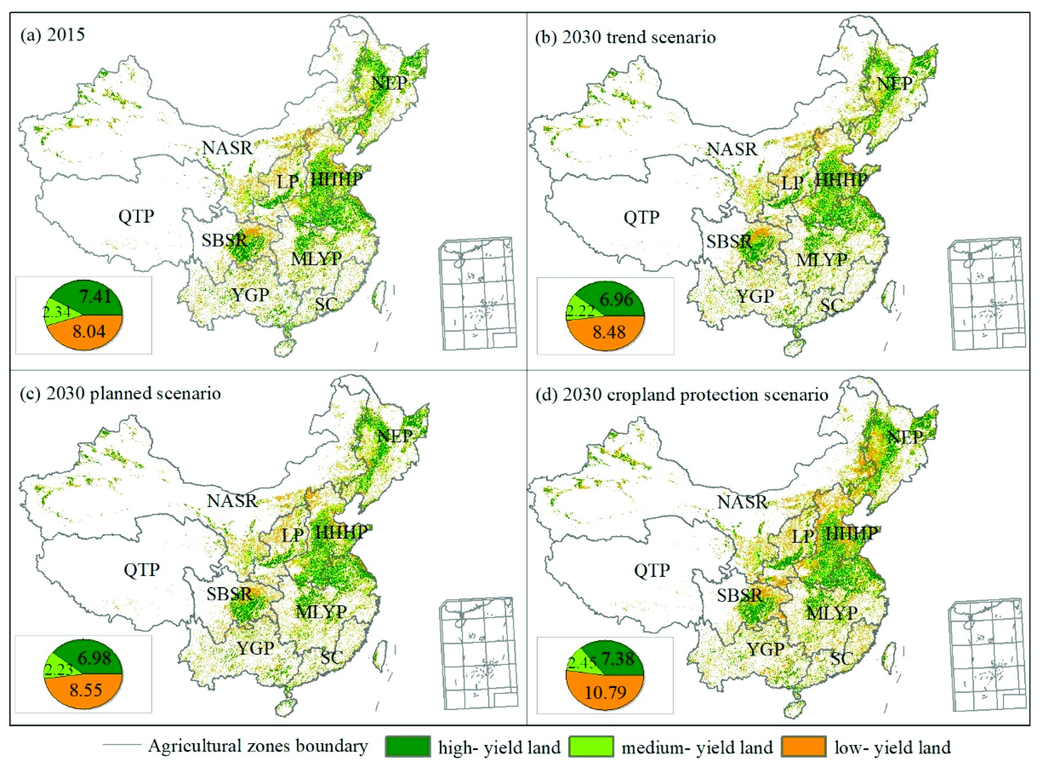
The potential crop yield data simulated by the GAEZ model at pixel level was applied to classify the cropland different quality grade. The spatial pattern of high-yield, medium-yield, and low-yield cropland in 2015 was presented in Figure 6a. The area of high-yield, medium-yield, and low-yield cropland would be 7.41 × 10⁵ km2, 2.35 × 10⁵ km2, and 8.04 × 10⁵ km2, respectively. The high-yield cropland would distribute mainly over Eastern Central, Northeast, and Central China. The spatial explicit cropland quality in 2030 under trend scenario, planned scenario, and cropland protection scenario were calculated based on the land used data predicted by the Dyna-CLUE model and crop yield data simulated by the GAEZ model. The spatial trends of cropland quality on a national scale is similar. However, local differences are clear between different scenarios (Figure 6). Under the trend scenario, the quantity of high-yield, medium-yield, and low-yield cropland was 6.96 × 10⁵ km2, 2.22 × 10⁵ km2, and 8.48 × 10⁵ km2, respectively. The high-yield cropland would be reduced under all three scenarios. At the national scale, the high-yield cropland would decrease 4.5 × 10⁴ km2, 4.3 × 10⁴ km2, and 0.3 × 10⁴ km2 for the trend scenario, the planned scenario, and the cropland protection scenario. The medium-yield cropland would reduce under the trend scenario and planned scenario, but would increase by 1.1 × 10⁴ km2 in the cropland protection scenario. The low-yield cropland would increase under all three scenarios.
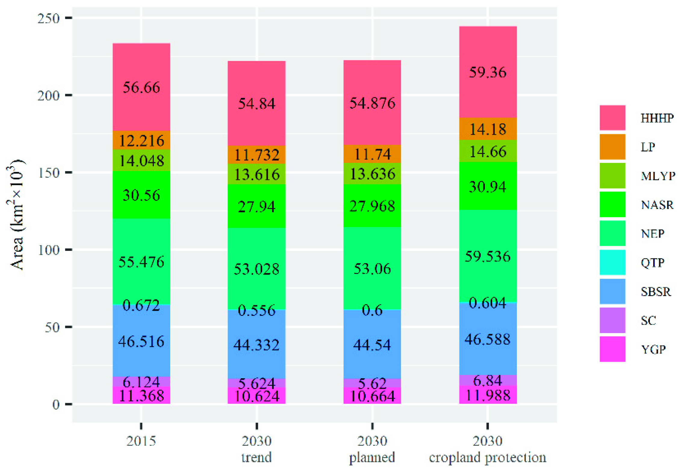
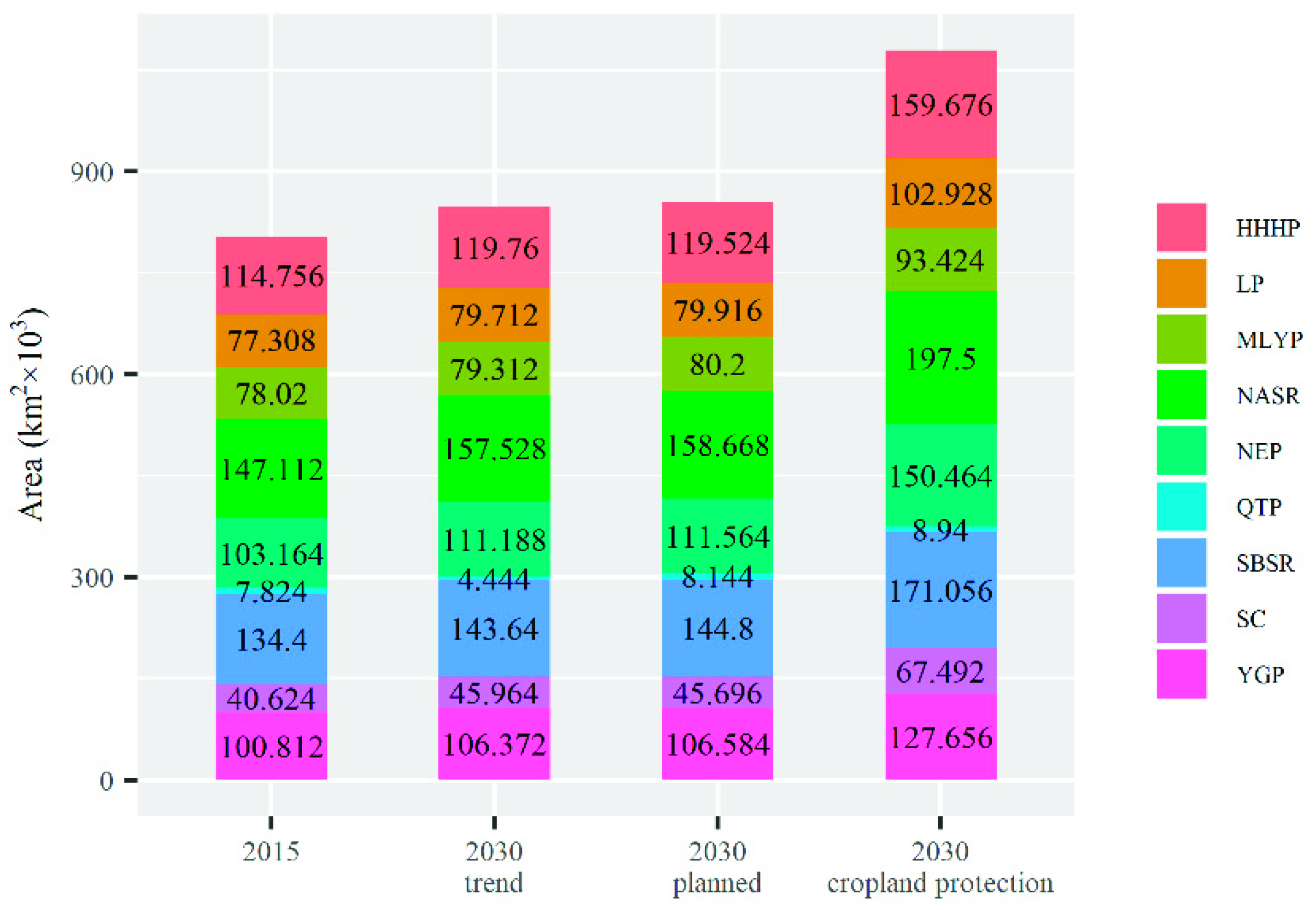
The cropland quality in 2030 under different scenarios for the nine agricultural zones was analyzed. The nine agricultural zones include the Northeast China Plain (NEP), The Northern arid and semiarid region (NASR), the Huang-Huai-Hai Plain (HHHP), the Loess Plateau (LP), the Qinghai Tibet Plateau (QTP), the Middle-lower Yangtze Plain (MLYP), the Sichuan Basin and surrounding regions (SBSR), the Yunnan-Guizhou Plateau (YGP), and Southern China (SC) (Figure 6).The quantity of high-yield, medium-yield, and low-yield cropland in 2030 under the three scenarios was calculated for each agricultural zone. The high-yield cropland would decrease in 2030 in most of the agricultural zones under trend scenario and planned scenario. Under cropland protection scenario, the high-yield cropland would increase in NEP, HHHP, and LP agricultural region, and would decrease in other zones (Figure 7). The medium-yield cropland would decrease in all zones under the trend scenario and planned scenario, and in the QTP zone under the cropland protection scenario. The increase of medium-yield cropland would occur in eight agricultural zones except the QTP zone (Figure 8). The low-yield cropland would increase in most of the agricultural zones in 2030 under the three scenarios except in the QTP zone in the trend scenario (Figure 9).
The consistency between the potential crop yield used in this study and the investigated actual yield was tested by Liu et al. [36]. The results showed that the cross-correlation coefficient is 0.82, and the standard deviation is 7.4 thousand tons [36]. Therefore, the potential crop yield agreed well with the actual yield data. Accordingly, the potential crop yield data does reflect the actual yield to a large extent. Lastly, the potential yield data, together with the spatially explicit land use data predicted by the Dyna-CLUE model, were used to calculate the changes in crop yield caused by land use change in China from 2015 to 2030. It was found that, for the trend scenario, the crop yield of all of the nine agricultural zones in 2030 decreased when compared with that in 2015 except for HHHP MLYP, and SC zones (Table 4). In the planned scenario, the differences of total crop yield for the whole country or the agricultural zones scales between 2015 and 2030 were small. The increase in crop yield was pronounced under the cropland protection scenario, and the increase was mainly distributed in the NEP and HHHP zones. In the two agricultural zones, crop yield increased by 2.66 × 10¹⁰ kg, which contributed 50% of the national total crop yield increase.
4. Discussion
4.1. Future Changes of Cropland Quantity
Land use strategies in 2030 were simulated according to the storylines of three land use change scenarios using the Dyna-CLUE model. As for the trend scenario, built-up land would increase, and a large part of the newly emerging built-up land would distribute around the existing built-up land. The cropland, grassland, and forest would decrease due to the pressure of human activities. As for the cropland protection scenario, the increase in cropland was due to the distinguishing characteristics. In the planned scenario, the decrease of cropland would be prevented compared with the trend scenario, and redline restriction was made by the government to guarantee the area of cropland against a decrease. However, the cropland under the planned scenario would not increase noticeably like the cropland protection scenario. The reason is that land use strategies made by the government laid emphasis not only on food security but also on the protection of the ecological environment. Ecological land was prohibited from reducing in order to promote the harmony of environmental sustainability and socioeconomic development in the planned scenario. Forest and grassland area would increase according to the land use planning. Therefore, the planned scenario emphasizes the concerted development of ecological land and cropland, and the cropland protection scenario is more efficient in protecting cropland.
4.2. Impacts of Land Use Change on Cropland Quality
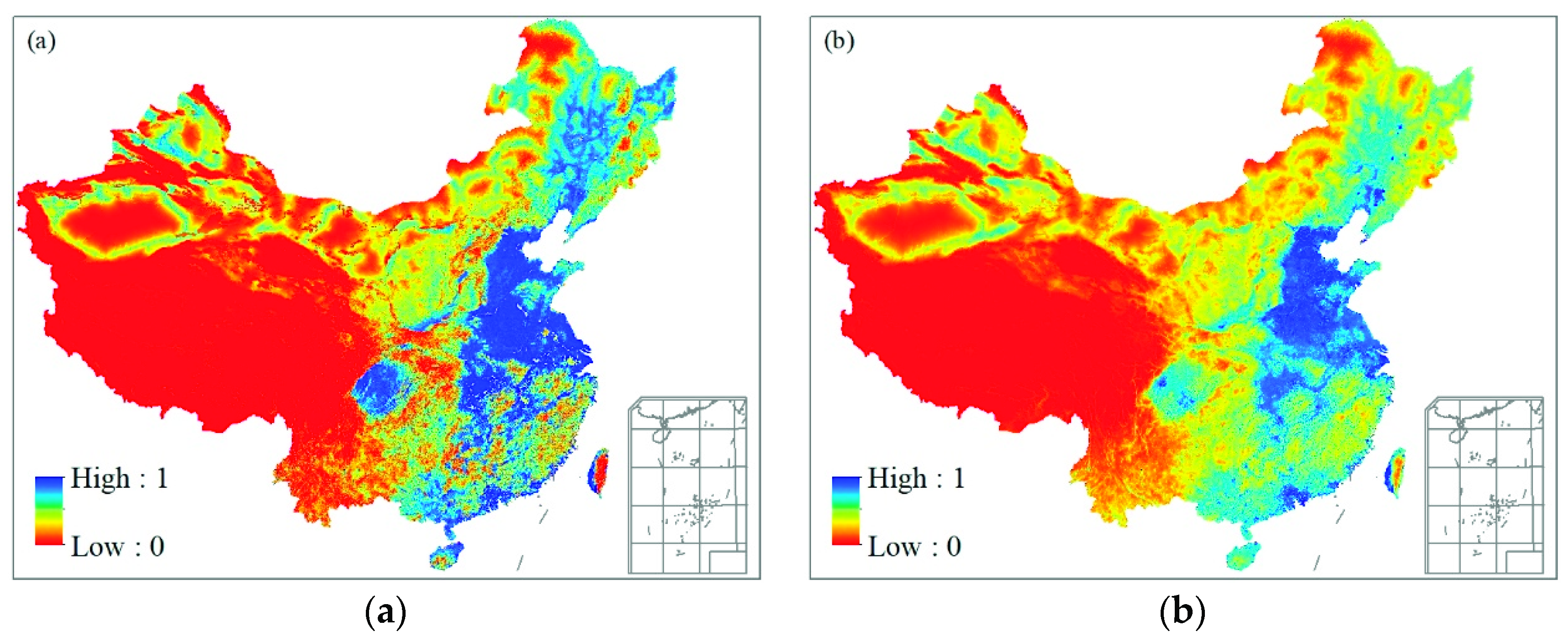
The spatial pattern of cropland quality on the pixel level in 2030 under different scenarios was also simulated. It helps decision-makers to further understand the location that should be protected and the location that can be developed. Typically, the converted lands for cropland have lower quality and were located in areas with low-yield cropland. In the planned scenario, the high-yield and medium-yield cropland would decrease and the low-yield cropland would increase. While in the cropland protection scenario, there would also be a small reduction of the high-yield cropland, and the medium-yield and low-yield cropland would increase. The reason is that urban development shares the same conditions as high-yield cropland, such as small slope, short distance to settlement, and water bodies. Therefore, the transfer probability of high-yield cropland is similar to urban built-up land to a large extent. Figure 10 shows the probability map of high-yield cropland and built-up land calculated through logistic regression between these two land use types and land use change driving factors. As a result, built-up land would occupy high quality cropland and pose a threat to food security in China. This situation is different in India, the United States, and Brazil, which will also lose large amounts of cropland. In these countries, large areas of cropland will be untouched during the process of built-up land expansion. Consequently, the domestic crop production would be less likely to be affected [3].
The findings of this research are in accordance with other existing studies. For example, Li et al. evaluated the impact of cropland shift on crop yield in China during 1990 and 2010. They found that fertile cropland was converted to built-up land, and more low-yield land was converted to cropland, which led to the decrease of the national average crop yield per unit area from 1990 to 2010 [32]. Yan et al. evaluated the effects of land use change on cropland productivity in China from 1990 to 2000. Their results demonstrated the newly compensated cropland for the occupation of cropland in the area, but the productivity of occupied cropland was 80% higher than that of the newly cropland [33]. He et al. also concluded that the total cropland net primary productivity decrease resulted from urban expansion in China from 1992 to 2015, which caused a threat to food security [34]. Song et al. found that urban expansion caused the loss of high-quality cropland for the period of 1986 to 2020 in Beijing [37]. Shi et al. found that large areas of fertile cropland were sacrificed to non-agricultural uses during the last decade in the Huang-Huai-Hai Plain of China [51]. Kong stated that some high-quality cropland have been built on or contaminated, and replaced by lower quality marginal land in the past years [52]. The comparison with regard to the future trend of cropland quality was unable to be carried out due to the lack of similar studies.
4.3. Future Crop Yield Change Induced by Land Use Change
The decrease in high-yield cropland and increase in low-yield cropland can be generalized as poor cropland for superior cropland. What would be the influence of such conversion on crop yield? How would this kind of influence vary across the agricultural zones of China? These problems were investigated in this study. This study showed that the total crop yield at the whole country scale would decrease in the trend scenario, remain stable in the planned scenario, and increase in the cropland protection scenario. The decline of crop yield would be controlled in all of the nine agricultural zones under the cropland protection scenario. The issue of food security has been of concern in China for many years [53]. The three development scenarios assessed in this research enables policy makers to have different options based on the local situations within each agricultural zone. For example, if the food provision is adequate, the planned scenario could be adopted, which also lays more emphasis on the protection and restoration of ecological land. The areas of forest, grassland, and water area would also achieve the aim of related forest, grassland, and water resource development plans in the planned scenario. On the other hand, the schemes of cropland protection scenario could be considered once the pressure of food supply becomes huge. The variation of crop yield was different on the agricultural zone scale, and recognizing these distinctions is conductive to the making of flexible land use management strategies for different zones. Good governance is necessary to meet the goals of cropland protection, environmental security, and economic development. It is crucial to lead future land use change to more sustainable means [54,55].
To get rid of crop yield change caused by other drivers than land use change, the potential crop yield dataset before land use change between 2015 and 2030 was used to estimate the original cropland quality. Thus, the fluctuation of crop yield during 2015 and 2030 was not taken into account. Will the decrease of crop yield in the trend scenario be relieved if the fluctuation of crop yield was considered? Herein, some investigations into the prospect of future crop production were performed. Crop yield increased substantially in China during the last two decades due to the consumption of a large amount of chemical fertilizer and increase of agricultural machinery power [56,57,58]. However, previous studies found that the yield increase of wheat, rice, and maize have decelerated or even stopped around 2010 in China. The reason may be that the gap between actual crop yield and yield potential are more likely to close [48]. Meanwhile, it is unreliable to increase the grain importation from the international market [59]. A decline in the global cereal yields was projected from 2010 to 2050 [60]. The global grain price index increased plenty and the grain supply from the world grain markets is finite [61]. Additionally, extensive independent studies have shown that climate change would reduce crop yield on a global scale [62,63]. Against this background, the problem of food security in China should be noticed and the government should take adaption measures and develop cropland protection strategies to enhance future sustainability development.
4.4. Uncertainty of the Assessments
There were some uncertainties in this research. First, land use data of year 2000 and 2015 were used to determine the trends of land use change in the trend scenario. The adopted approach assumed that there was no abrupt turning point in the area of each land use type from 2000 to 2015. However, in reality, the actual land use change graph can be flat at the end of the 15-year period (for 2015) or even, reaching a peak earlier (between 2000 and 2015), already have a real downward trend (despite the demonstrated upward trend). Therefore, using data from at least three periods of time instead of two would greatly reduce the size of the forecast error. Second, the pixel size of the land use data and crop yield data is 1 × 1 km. Thus, mixed pixels bring about errors in the quantity of each land use. Third, the validation of the land use prediction model is practical only for the past land use data. The simulated and actual land use data in 2015 were compared, and the good validation results can indicate the validity of the allocation algorithms within the model. Fourth, the fluctuations of land use change driving factors from 2015 to 2030 were not taken into consideration in the process of simulation. Although Dyna-CLUE is one of the most extensively used model in predicting land use change, some uncertainty in the simulated results may still exist. For example, some land use change driving factors may not be captured. Nevertheless, the assessment performed in this research is still worthwhile. It has managed to picture the details of the cropland quantity and crop yield variation caused by land use change in the next two decades in China. The results are crucial for sustainable agriculture and food security.
5. Conclusions
This study simulated land use change from 2015 to 2030 under the trend scenario, the planned scenario, and the cropland protection scenario using the Dyna-CLUE model. Cropland quality grade was calculated based on a potential crop yield dataset at the pixel level. The impacts of future land use change on cropland quality and crop yield at national and agricultural zones scales were investigated. This research found that, under the trend scenario, the area of cropland and the crop yield would continue to decrease. The high-yield and medium-yield cropland would decrease and the low-yield cropland would increase. Under the planned scenario, the arbitrary occupation of cropland would be prohibited, and the crop yield would remain unchanged. The high-yield and medium-yield cropland would decrease and the low-yield cropland would increase. Under the cropland protection scenario, the cropland area and the crop yield would increase, and there would be a small reduction of the high-yield cropland, and the medium-yield and low-yield cropland would increase. The converted lands for cropland would mainly occur in Northeastern and Northern China, and the reduced high-quality cropland would mainly be occupied by the built-up land. The Dyna-CLUE model has been successfully used in various regions. Therefore, the method of this study could be applied in other study areas easily with specific development scenarios.
As noted above, the food production would be sustainable only for the two main drivers, which include cropland quality and quantity, which are under control. Both the planned scenario and cropland protection scenario fail to reverse the reduction of high-yield cropland, even though they present much fewer losses of high-quality cropland than the trend scenario. This suggests that land use policies of China should take into account both the quantity and quality of cropland. For example, the Farmland Requisition-Compensation Balance policy, which aims to offset losses in cropland area to built-up land with gains in new cropland, should require a quality balance rather than solely a quantity balance. The findings in this study have substantiated that high-yield cropland resources are limited in China and a large portion of the new gained cropland would be low-yield cropland, even under the cropland protection scenario. Therefore, upgrading medium-yield and low-yield cropland is a critical step toward the sustainable management of cropland and a deep insight into it should be taken by the policy-makers and scientists. Some projects on improving lower quality cropland have been undertaken by different ministries. The cost is merited and more fund and money should be put on these projects. Furthermore, the government needs to establish a payment system to reinforce the protection and reclamation of high-yield cropland.
Land use data with finer spatial-temporal resolution will be applied in the next research study, which can improve the accuracy of future prediction. Meanwhile, the next study will link the Dyna-CLUE with a production efficiency model (GLOPEM-CEVSA) and machine learning approaches to estimate the influence of the yield gap between potential and actual crop yield on food security in the future.
Author Contributions
Conceptualization, M.W. Methodology, X.S. Software, Z.F. Validation, Z.F. Formal analysis, T.Y. Resources, M.W. Data curation, X.S. Writing—original draft preparation, M.W. Writing—review and editing, X.S. Supervision, X.S. Funding acquisition, M.W.
Funding
The Humanities and Social Sciences Foundation of the Ministry of Education in China (16YJCZH098) provided financial support for this research.
Conflicts of Interest
The authors declare no conflict of interest.
References
- FAO. The State of the World’s Land and Water Resources for Food and Agriculture; Earthscan Publications: London, UK, 2011. [Google Scholar]
- Deng, X.; Gibson, J.; Wang, P. Management of trade-offs between cultivated land conversions and land productivity in Shandong Province. J. Clean. Prod. 2017, 142, 767–774. [Google Scholar] [CrossRef]
- Bren, D.A.C.; Reitsma, F.; Baiocchi, G.; Barthel, S.; Güneralp, B.; Erb, K.H.; Haberl, H.; Creutzig, F.; Seto, K.C. Future urban land expansion and implications for global croplands. Proc. Natl. Acad. Sci. USA 2016, 114, 8939–8944. [Google Scholar] [CrossRef] [PubMed] [Green Version]
- Tang, J.; Di, L. Past and Future Trajectories of Farmland Loss Due to Rapid Urbanization Using Landsat Imagery and the Markov-CA Model: A Case Study of Delhi, India. Remote Sens. 2019, 11, 180. [Google Scholar] [CrossRef]
- Lasanta, T.; Arnaez, J.; Pascual, N.; Ruiz-Flano, P.; Errea, M.P.; Lana-Renault, N. Space-time process and drivers of land abandonment in Europe. Catena 2017, 149, 810–823. [Google Scholar] [CrossRef]
- Schulp, C.J.E.; Levers, C.; Kuemmerle, T.; Tieskens, K.F.; Verburg, P.H. Mapping and modelling past and future land use change in Europe’s cultural landscapes. Land Use Policy 2019, 80, 332–344. [Google Scholar] [CrossRef]
- Ren, Y.; Lü, Y.; Comber, A.; Fu, B.; Harris, P.; Wu, L. Spatially explicit simulation of land use/land cover changes: Current coverage and future prospects. Earth-Sci. Rev. 2019, 190, 398–415. [Google Scholar] [CrossRef]
- Fondevilla, C.; Colomer, M.À.; Fillat, F.; Tappeiner, U. Using a new PDP modelling approach for land-use and land-cover change predictions: A case study in the Stubai Valley (Central Alps). Ecol. Model. 2016, 322, 101–114. [Google Scholar] [CrossRef] [Green Version]
- Bao, J.; Gao, S.; Ge, J. Dynamic land use and its policy in response to environmental and social-economic changes in China: A case study of the Jiangsu coast (1750–2015). Land Use Policy 2019, 82, 169–180. [Google Scholar] [CrossRef]
- Murray-Rust, D.; Rieser, V.; Robinson, D.T.; Milicic, V.; Rounsevell, M. Agent-based modelling of land use dynamics and residential quality of life for future scenarios. Environ. Model. Softw. 2013, 46, 75–89. [Google Scholar] [CrossRef]
- Liu, J.; Li, J.; Qin, K.; Zhou, Z.; Yang, X.; Li, T. Changes in land-uses and ecosystem services under multi-scenarios simulation. Sci. Total Environ. 2017, 586, 522–526. [Google Scholar] [CrossRef]
- Seto, K.C.; Burak, G.; Hutyra, L.R. Global forecasts of urban expansion to 2030 and direct impacts on biodiversity and carbon pools. Proc. Natl. Acad. Sci. USA 2012, 109, 16083–16088. [Google Scholar] [CrossRef] [PubMed] [Green Version]
- Liu, F.; Zhang, Z.; Zhao, X.; Wang, X.; Zuo, L.; Wen, Q.; Yi, L.; Xu, J.; Hu, S.; Liu, B. Chinese cropland losses due to urban expansion in the past four decades. Sci. Total Environ. 2019, 650, 847–857. [Google Scholar] [CrossRef] [PubMed]
- Fukase, E.; Martin, W. Who will feed China in the 21st century? Income growth and food demand and supply in China. J. Agric. Econ. 2016, 67, 3–23. [Google Scholar] [CrossRef]
- Akbar, T.A.; Hassan, Q.K.; Ishaq, S.; Batool, M.; Butt, H.J.; Jabbar, H. Investigative spatial distribution and modelling of existing and future urban land changes and its impact on urbanization and economy. Remote Sens. 2019, 11, 105. [Google Scholar] [CrossRef]
- Trivedi, H.V.; Singh, J.K. Application of grey system theory in the development of a runoff prediction model. Biosyst. Eng. 2005, 92, 521–526. [Google Scholar] [CrossRef]
- Xu, X.; Du, Z.; Hong, Z. Integrating the system dynamic and cellular automata models to predict land use and land cover change. Int. J. Appl. Earth Obs. Geoinf. 2016, 52, 568–579. [Google Scholar] [CrossRef]
- Trisurat, Y.; Shirakawa, H.; Johnston, J.M. Land-use/land-cover change from socio-economic drivers and their impact on biodiversity in Nan Province, Thailand. Sustainability 2019, 11, 649. [Google Scholar] [CrossRef]
- Tian, G.; Ma, B.; Xu, X.; Liu, X.; Xu, L.; Liu, X.; Lin, X.; Kong, L. Simulation of urban expansion and encroachment using cellular automata and multi-agent system model-A case study of Tianjin metropolitan region, China. Ecol. Indic. 2016, 70, 439–450. [Google Scholar] [CrossRef]
- Samie, A.; Deng, X.; Jia, S.; Chen, D. Scenario-based simulation on dynamics of land-use-land-cover change in Punjab Province, Pakistan. Sustainability 2017, 9, 1285. [Google Scholar] [CrossRef]
- Jia, Z.; Ma, B.; Zhang, J.; Zeng, W. Simulating spatial-temporal changes of land-use based on ecological redline restrictions and landscape driving factors: A case study in Beijing. Sustainability 2018, 10, 1299. [Google Scholar] [CrossRef]
- Verburg, P.H.; Overmars, K.P. Combining top-down and bottom-up dynamics in land use modeling: Exploring the future of abandoned farmlands in Europe with the Dyna-CLUE model. Landsc. Ecol. 2009, 24, 1167–1181. [Google Scholar] [CrossRef]
- Sun, X.; Yue, T.; Meng, W.; Fan, Z.; Liu, F. Effects of land use planning on aboveground vegetation biomass in China. Environ. Earth Sci. 2015, 73, 6553–6564. [Google Scholar] [CrossRef]
- Sahoo, S.; Sil, I.; Dhar, A.; Debsarkar, A.; Das, P.; Kar, A. Future scenarios of land-use suitability modeling for agricultural sustainability in a river basin. J. Clean. Prod. 2018, 205, 313–328. [Google Scholar] [CrossRef]
- Verburg, P.H.; van Berkel, D.B.; van Doorn, A.M.; van Eupen, M.; van den Heiligenberg, H. Trajectories of land use change in Europe: A model-based exploration of rural futures. Landsc. Ecol. 2010, 25, 217–232. [Google Scholar] [CrossRef]
- Verburg, P.H.; Eickhout, B.; van Meijl, H. A multi-scale, multi-model approach for analyzing the future dynamics of European land use. Ann. Reg. Sci. 2008, 42, 57–77. [Google Scholar] [CrossRef]
- Wang, Y.; Li, X.; Zhang, Q.; Li, J.; Zhou, X. Projections of future land use changes: Multiple scenarios-based impacts analysis on ecosystem services for Wuhan city, China. Ecol. Indic. 2018, 94, 430–445. [Google Scholar] [CrossRef]
- Stürck, J.; Schulp, C.J.E.; Verburg, P.H. Spatio-temporal dynamics of regulating ecosystem services in Europe—The role of past and future land use change. Appl. Geogr. 2015, 63, 121–135. [Google Scholar] [CrossRef]
- Jin, T. Effects of cultivated land use on temporal-spatial variation of grain production in China. J. Nat. Resour. 2014, 29, 911–919. [Google Scholar]
- Wang, J.Y.; Liu, Y.S. The changes of grain output center of gravityand its driving forces in China since 1990. Resour. Sci. 2009, 31, 1188–1194. [Google Scholar]
- Song, W.; Pijanowski, B.C. The effects of China’s cultivated land balance program on potential land productivity at a national scale. Appl. Geogr. 2014, 46, 158–170. [Google Scholar] [CrossRef]
- Li, Y.; Li, X.; Tan, M.; Xue, W.; Xin, L. The impact of cultivated land spatial shift on food crop production in China, 1990–2010. Land Degrad. Dev. 2018, 29, 1652–1659. [Google Scholar] [CrossRef]
- Yan, H.; Liu, J.; Huang, H.Q.; Tao, B.; Cao, M. Assessing the consequence of land use change on agricultural productivity in China. Glob. Planet. Chang. 2009, 67, 13–19. [Google Scholar] [CrossRef]
- He, C.; Liu, Z.; Xu, M.; Ma, Q.; Dou, Y. Urban expansion brought stress to food security in China: Evidence from decreased cropland net primary productivity. Sci. Total Environ. 2017, 576, 660–670. [Google Scholar] [CrossRef] [PubMed]
- Wang, C.; Sun, X.; Wang, M.; Wang, J.; Ding, Q. Chinese cropland quality and its temporal and spatial changes due to urbanization in 2000–2015. J. Resour. Ecol. 2019, 10, 174–183. [Google Scholar]
- Liu, L.; Xu, X.; Chen, X. Assessing the impact of urban expansion on potential crop yield in China during 1990–2010. Food Secur. 2015, 7, 33–43. [Google Scholar] [CrossRef]
- Song, W.; Pijanowski, B.C.; Tayyebi, A. Urban expansion and its consumption of high-quality farmland in Beijing, China. Ecol. Indic. 2015, 54, 60–70. [Google Scholar] [CrossRef]
- Lu, X.; Shi, Y.; Chen, C.; Yu, M. Monitoring cropland transition and its impact on ecosystem services value in developed regions of China: A case study of Jiangsu Province. Land Use Policy 2017, 69, 25–40. [Google Scholar] [CrossRef]
- Lin, L.; Ye, Z.; Gan, M.; Shahtahmassebi, A.R.; Weston, M.; Deng, J.; Lu, S.; Wang, K. Quality perspective on the dynamic balance of cultivated land in Wenzhou, China. Sustainability 2017, 9, 95. [Google Scholar] [CrossRef]
- Liu, J.; Xu, X.; Zhuang, D.; Gao, Z. Impacts of LUCC processes on potential land productivity in China in the 1990s. Sci. China 2005, 48, 1259–1269. [Google Scholar] [CrossRef]
- Song, W.; Liu, M. Farmland conversion decreases regional and national land quality in China. Land Degrad. Dev. 2017, 28, 459–471. [Google Scholar] [CrossRef]
- Liu, J.Y.; Liu, M.L.; Zhuang, D.F.; Zhang, Z.X.; Deng, X.Z. Study on spatial pattern of land-use change in China during 1995–2000. Sci. China 2003, 46, 373–384. [Google Scholar]
- Meng, W.; Sun, X. Potential impact of land use change on ecosystem services in China. Environ. Monit. Assess. 2016, 188, 1–13. [Google Scholar]
- Tang, J.; Wang, L.; Yao, Z. Spatio-temporal urban landscape change analysis using the Markov chain model and a modified genetic algorithm. Int. J. Remote Sens. 2007, 28, 3255–3271. [Google Scholar] [CrossRef]
- National General Land Use Planning Outline of China (2016–2030). Available online: http://www.gov.cn/zhengce/content/2017-02/04/content_5165309.htm (accessed on 1 March 2017).
- Jiang, W.; Chen, Z.; Lei, X.; Jia, K.; Yongfeng, W.U. Simulating urban land use change by incorporating an autologistic regression model into a CLUE-S model. J. Geogr. Sci. 2015, 25, 836–850. [Google Scholar] [CrossRef] [Green Version]
- Moulds, S.; Buytaert, W.; Mijic, A. An open and extensible framework for spatially explicit land use change modelling: The lulcc R package. Geosci. Mod. Dev. 2015, 8, 3215–3229. [Google Scholar] [CrossRef]
- Pontius, R.G.; Peethambaram, S.; Castella, J.-C. Comparison of three maps at multiple resolutions: A case study of land change simulation in Cho Don District, Vietnam. Ann. Assoc. Am. Geogr. 2011, 101, 45–62. [Google Scholar] [CrossRef]
- Chen, H.; Pontius, R.G. Diagnostic tools to evaluate a spatial land change projection along a gradient of an explanatory variable. Landsc. Ecol. 2010, 25, 1319–1331. [Google Scholar] [CrossRef]
- Varga, O.G.; Pontius, R.G.; Singh, S.K.; Szabó, S. Intensity analysis and the figure of Merit’s components for assessment of a cellular automata—Markov simulation model. Ecol. Indic. 2019, 101, 933–942. [Google Scholar] [CrossRef]
- Shi, W.; Tao, F.; Liu, J. Changes in quantity and quality of cropland and the implications for grain production in the Huang-Huai-Hai Plain of China. Food Secur. 2013, 5, 69–82. [Google Scholar] [CrossRef]
- Kong, X. China must protect high-quality arable land. Nature 2014, 506, 7. [Google Scholar] [CrossRef]
- Xing, W.; Zhao, Z.; Peijun, S.; Pin, W.; Yi, C.; Xiao, S.; Fulu, T. Is yield increase sufficient to achieve food security in China? PLoS ONE 2015, 10, e0116430. [Google Scholar]
- Koroso, N.H.; Van der Molen, P.; Tuladhar, A.M.; Zevenbergen, J.A. Does the Chinese market for urban land use rights meet good governance principles? Land Use Policy 2013, 30, 417–426. [Google Scholar] [CrossRef]
- Jiang, L.; Deng, X.; Seto, K.C. Multi-level modeling of urban expansion and cultivated land conversion for urban hotspot counties in China. Landsc. Urban Plan. 2012, 108, 131–139. [Google Scholar] [CrossRef]
- Chen, X.; Cui, Z.; Fan, M.; Vitousek, P.; Zhao, M.; Ma, W.; Wang, Z.; Zhang, W.; Yan, X.; Yang, J.; et al. Producing more grain with lower environmental costs. Nature 2014, 514, 486. [Google Scholar] [CrossRef] [PubMed]
- Tian, H.; Lu, C.; Melillo, J.; Ren, W.; Huang, Y.; Xu, X.; Liu, M.; Zhang, C.; Chen, G.; Pan, S.; et al. Food benefit and climate warming potential of nitrogen fertilizer uses in China. Environ. Res. Lett. 2012, 7, 044020. [Google Scholar] [CrossRef]
- Wang, X.; Cai, D.; Hoogmoed, W.B.; Oenema, O. Regional distribution of nitrogen fertilizer use and N-saving potential for improvement of food production and nitrogen use efficiency in China. J. Sci. Food Agric. 2011, 91, 2013–2023. [Google Scholar] [CrossRef]
- Suweis, S.; Carr, J.A.; Maritan, A.; Rinaldo, A.; D’Odorico, P. Resilience and reactivity of global food security. Proc. Natl. Acad. Sci. USA 2015, 112, 6902–6907. [Google Scholar] [CrossRef] [PubMed] [Green Version]
- Wheeler, T.; von Braun, J. Climate change impacts on global food security. Science 2013, 341, 508–513. [Google Scholar] [CrossRef]
- Godfray, H.C.; Beddington, J.R.; Crute, I.R.; Haddad, L.; Lawrence, D.; Muir, J.F.; Pretty, J.; Robinson, S.; Thomas, S.M.; Toulmin, C. Food security: The challenge of feeding 9 billion people. Science 2010, 327, 812–818. [Google Scholar] [CrossRef]
- Zhao, C.; Liu, B.; Piao, S.; Wang, X.; Lobell, D.B.; Huang, Y.; Huang, M.; Yao, Y.; Bassu, S.; Ciais, P. Temperature increase reduces global yields of major crops in four independent estimates. Proc. Natl. Acad. Sci. USA 2017, 114, 9326. [Google Scholar] [CrossRef]
- Cynthia, R.; Joshua, E.; Delphine, D.; Ruane, A.C.; Christoph, M.; Almut, A.; Boote, K.J.; Christian, F.; Michael, G.; Nikolay, K. Assessing agricultural risks of climate change in the 21st century in a global gridded crop model intercomparison. Proc. Natl. Acad. Sci. USA 2014, 111, 3268–3273. [Google Scholar]
Figure 1.
Flowchart of the procedure of this study.
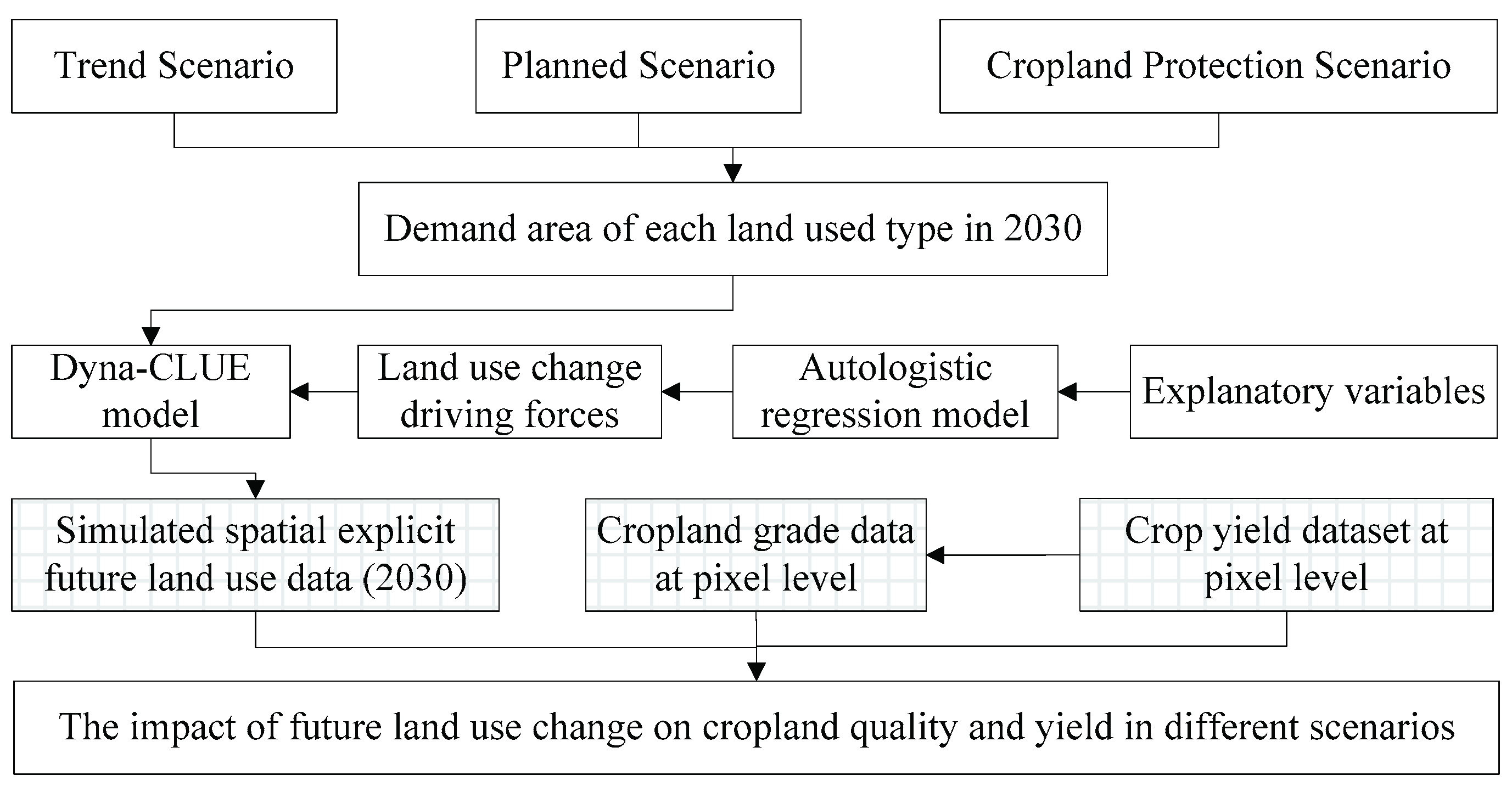
Figure 2.
Grid map of driving factors for the land use simulation: (a) elevation, (b) slope, (c) aspect, (d) silt soil percent, (e) clay soil percent, (f) sand soil percent, (g) soil depth, (h) soil pH, (i) drainage, (j) annual average temperature, (k) annual total precipitation, (l) radiation, (m) Gross Domestic Product (GDP), (n) population density, and (o) distance to the main roads.
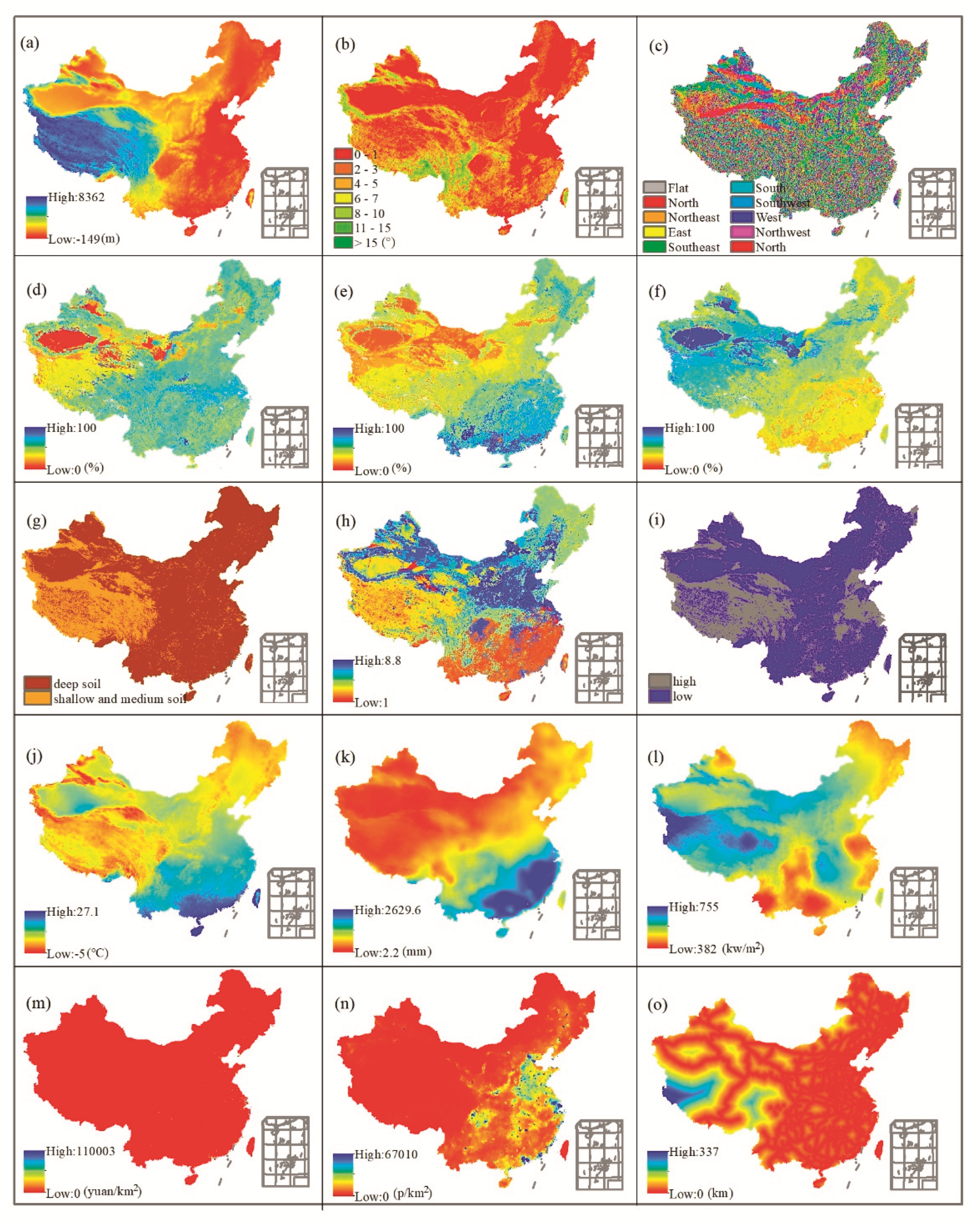
Figure 3.
The distribution of the natural reserve in China. Inset picture shows the location of China.
Figure 3.
The distribution of the natural reserve in China. Inset picture shows the location of China.
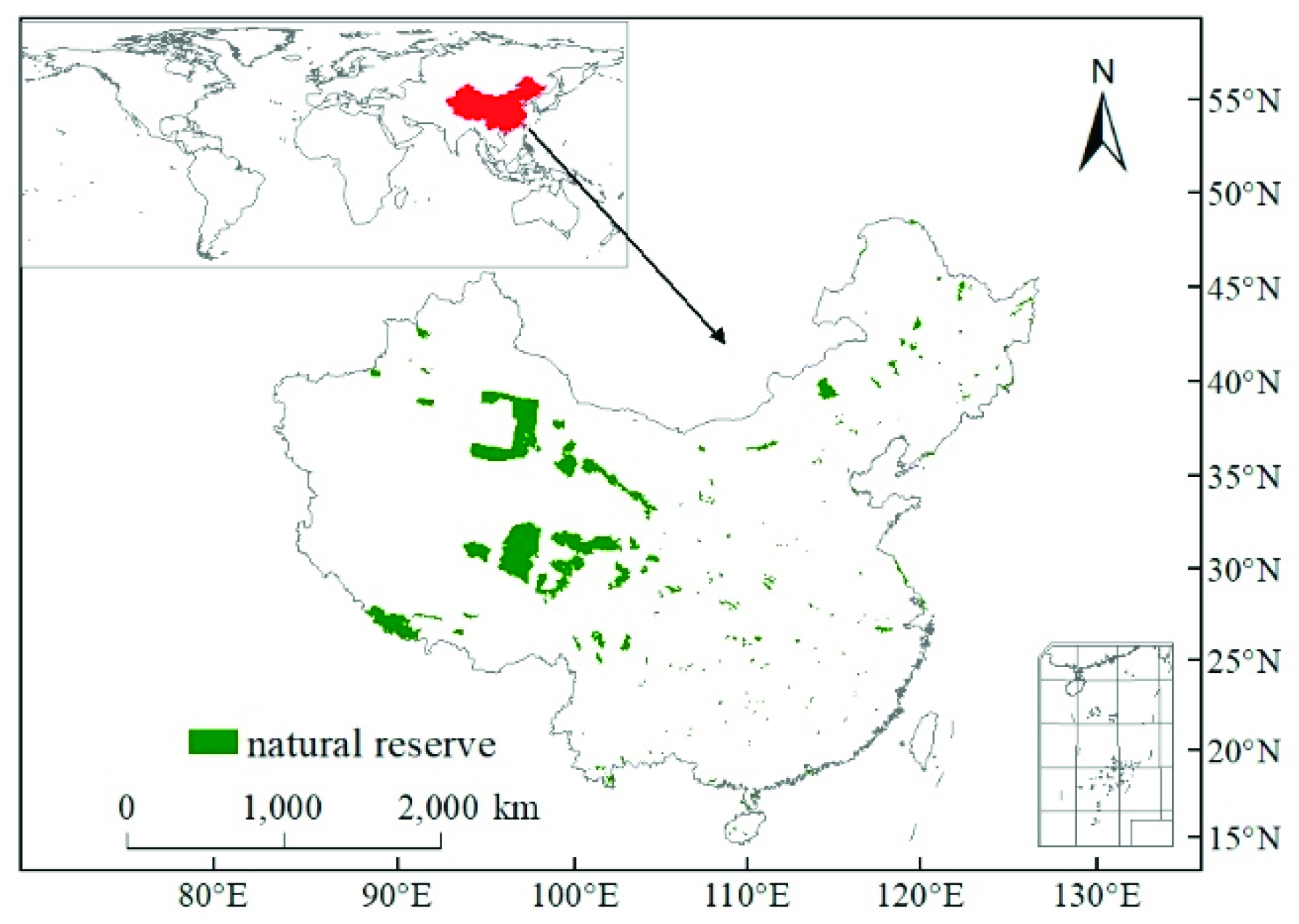
Figure 4.
(a) Map of components of agreement and disagreement. Inset histogram chart shows the value of FOM’s components as a percentage of the spatial extent (unit: %) (b) Total disagreement and hits.
Figure 4.
(a) Map of components of agreement and disagreement. Inset histogram chart shows the value of FOM’s components as a percentage of the spatial extent (unit: %) (b) Total disagreement and hits.

Figure 5.
Spatial pattern of cropland in 2015 (a) and predicted cropland distributions in 2030 under trend scenario (b), planned scenario (c), and cropland protection scenario (d).
Figure 5.
Spatial pattern of cropland in 2015 (a) and predicted cropland distributions in 2030 under trend scenario (b), planned scenario (c), and cropland protection scenario (d).
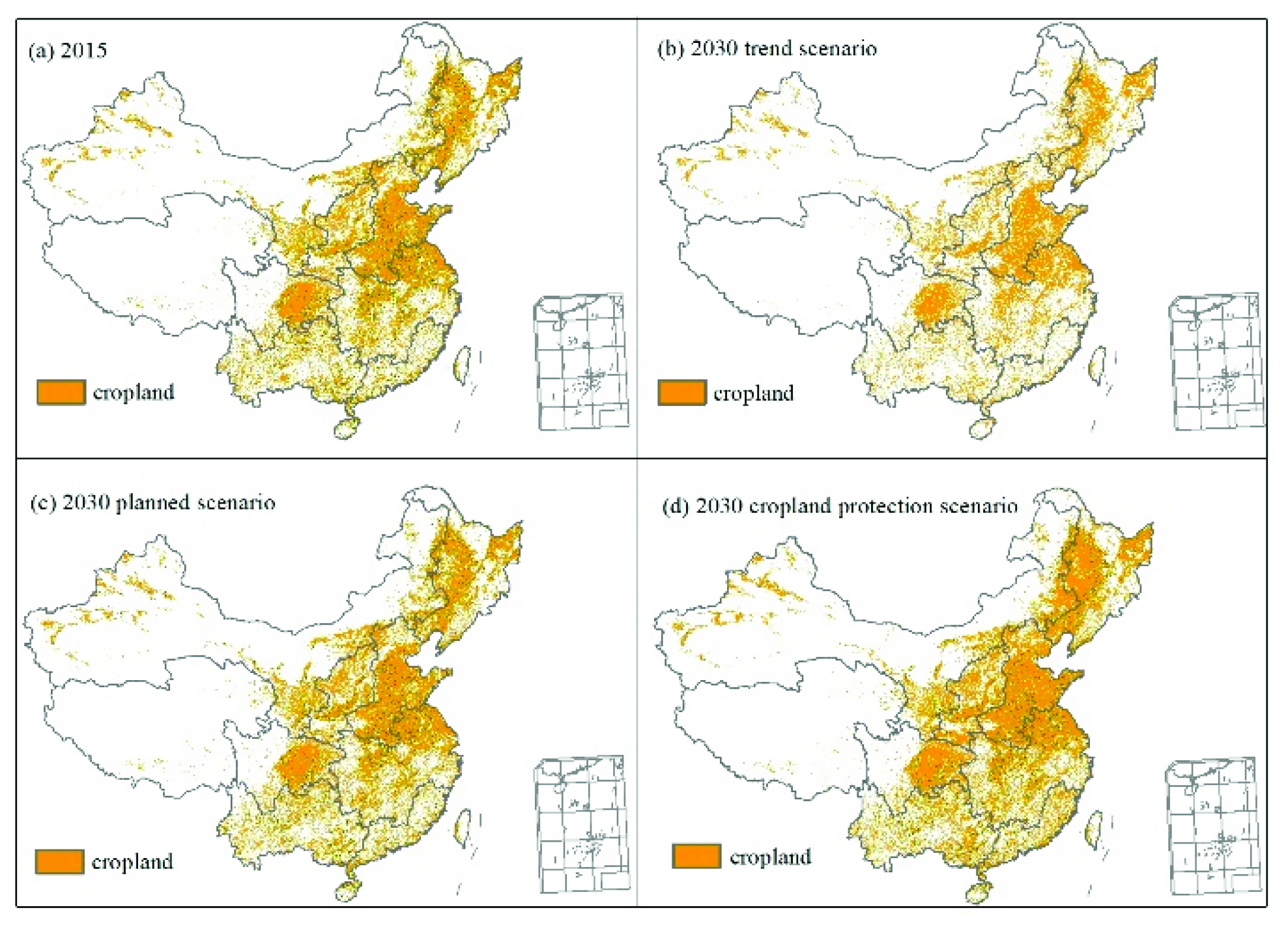
Figure 6.
Quality maps in 2015 (a) and simulated cropland quality under different scenarios in 2030. (b) Trend scenario, (c) planned scenario, and (d) cropland protection scenario. Agricultural zones are labeled using abbreviations: Northeast China Plain (NEP), The Northern arid and semiarid region (NASR), the Huang-Huai-Hai Plain (HHHP), the Loess Plateau (LP), the Qinghai Tibet Plateau (QTP), the Middle-lower Yangtze Plain (MLYP), the Sichuan Basin and surrounding regions (SBSR), the Yunnan-Guizhou Plateau (YGP), and Southern China (SC). The inset pie chart show the total area of high-yield, medium-yield, and low-yield cropland (unit: km2 × 105).

Figure 7.
The area of high-yield cropland in nine agricultural zones of China.

Figure 8.
The area of medium-yield cropland in nine agricultural zones of China.

Figure 9.
The area of low-yield cropland in nine agricultural zones of China.

Figure 10.
The occurrence probability maps for high-yield cropland (a) and built-up land (b).

Table 1.
Prediction of land use requirements for 2030 under different scenarios (km2).
| Scenarios | Cropland | Built-Up | Grassland | Forest | Water Area | Unused |
|---|---|---|---|---|---|---|
| 2015 | 1,780,228 | 216,164 | 2,978,288 | 2,231,256 | 265,568 | 1,980,640 |
| Trend scenario | 1,767,860 | 262,684 | 2,956,316 | 2,229,736 | 270,596 | 1,964,952 |
| Planned scenario | 1,778,857 | 260,112 | 2,976,812 | 2,469,580 | 265,144 | 1,701,638 |
| Cropland protection scenario | 2,067,685 | 216,038 | 2,868,192 | 2,226,214 | 267,180 | 1,806,832 |
Table 2.
Use conversion rules under different scenarios *.
| Land Use | Built-Up | Cropland | Grassland | Forest | Water Area | Unused |
|---|---|---|---|---|---|---|
| Built-up | 1,1,1 | 1,1,1 | 1,1,1 | 1,1,1 | 1,1,1 | 1,1,1 |
| Cropland | 1,1,1 | 1,1,1 | 1,1,1 | 1,1,1 | 1,1,0 | 1,1,0 |
| Grassland | 1,18,18 | 1,18,18 | 1,1,1 | 1,1,0 | 1,0,0 | 1,1,1 |
| Forest | 1,18,18 | 1,18,18 | 1,1,1 | 1,1,1 | 1,0,0 | 1,0,0 |
| Water area | 1,0,0 | 1,0,0 | 1,0,0 | 1,0,0 | 1,1,1 | 1,0,0 |
| Unused | 1,1,1 | 1,1,1 | 1,1,1 | 1,1,1 | 1,1,1 | 1,1,1 |
Note: * The conversion values in the table are for trend scenario, planned scenario, and cropland protection scenario, respectively, from left to right.
Table 3.
Logistic regression coefficients of each land use type.
| Variables | Built-Up | Cropland | Grassland | Forest | Water Area |
|---|---|---|---|---|---|
| Slope | −0.003 ** | −0.001 ** | 0.002 ** | −9.0810−4 ** | |
| Elevation | −0.00097 ** | −9.34 × 10⁻⁴ ** | 5.32 × 10⁻⁴ | −4.74 × 10⁻⁴ ** | −6.47 × 10⁻⁵ ** |
| Aspect | −3.8 × 10⁻⁷ ** | −5.42 × 10⁻⁷ ** | −1.19 × 10⁻⁷ ** | ||
| Silt soil percent | −2.30786 | −1.33597 | 1.09586 | 1.29462 | |
| Sand soil percent | −2.55572 | −1.48002 | 0.68501 * | 1.67125 | |
| Clay soil percent | −2.64192 | −1.68801 | 0.94395 | 1.83934 | |
| Sallow and medium soil | −1.40601 * | −0.26737 * | |||
| Deep soil | 0.95846 | ||||
| pH | 0.02412 ** | 0.02643 ** | 0.02278 ** | −0.02242 ** | |
| Soil organic carbon | −0.00035 ** | −2.64 × 10⁻⁴ ** | 0.00119 ** | 0.00227 ** | |
| High drainage | −0.11215 * | 1.26173 * | |||
| Low drainage | −0.56816 * | −0.6355 * | 0.701 * | ||
| Temperature | 0.00499 ** | −0.00252 ** | −0.00276 ** | −0.01259 ** | −0.00478 ** |
| Precipitation | 8.13 × 10⁻⁵ ** | −7.52 × 10⁻⁵ ** | 2.53 × 10⁻⁴ ** | 6.32 × 10⁻⁵ ** | |
| Radiation | 1.35 × 10⁻⁶ ** | 8.45 × 10⁻⁷ ** | −2.41 × 10⁻⁶ ** | −2.88 × 10⁻⁶ ** | 2.10 × 10⁻⁶ ** |
| GDP | 0.00006 ** | 2.04 × 10⁻⁵ ** | −5.17 × 10⁻⁵ ** | −3.00 × 10⁻⁵ ** | 6.74 × 10⁻⁵ ** |
| Distance to main roads | −5.68 × 10⁻⁷ ** | −4.02 × 10⁻⁶ ** | 6.01 × 10⁻⁶ ** | −9.12 × 10⁻⁶ ** | −2.36 × 10⁻⁶ ** |
| Population | 0.00068 * | 2.00 × 10⁻⁴ ** | −8.00 × 10⁻⁴ ** | −6.20 × 10⁻⁵ ** | −4.38 × 10⁻⁴ ** |
| ROC | 0.92 | 0.93 | 0.81 | 0.91 | 0.80 |
Note: * and ** represent significance at 0.01 and 0.05 level, respectively.
Table 4.
Crop yield in 2015 and in 2030 under three scenarios in each agricultural zone.
| Agricultural Zone | 2015 | 2030 Trend Scenario | 2030 Planned Scenario | 2030 Cropland Protection Scenario | ||||
|---|---|---|---|---|---|---|---|---|
| Amount (kg × 1010) | Percentage * (%) | Amount (kg × 1010) | Percentage (%) | Amount (kg × 1010) | Percentage (%) | Amount (kg × 1010) | Percentage (%) | |
| NEP | 13.62 | 18.63 | 13.61 | 18.65 | 13.62 | 18.63 | 14.82 | 18.90 |
| NASR | 6.99 | 9.57 | 6.98 | 9.57 | 6.99 | 9.57 | 7.63 | 9.73 |
| HHHP | 20.15 | 27.57 | 20.15 | 27.62 | 20.15 | 27.56 | 21.60 | 27.53 |
| LP | 3.75 | 5.13 | 3.74 | 5.13 | 3.75 | 5.13 | 4.29 | 5.47 |
| QTP | 0.13 | 0.18 | 0.11 | 0.15 | 0.13 | 0.18 | 0.13 | 0.17 |
| MLYP | 5.63 | 7.71 | 5.63 | 7.72 | 5.63 | 7.71 | 5.87 | 7.48 |
| SBSR | 18.57 | 25.41 | 18.48 | 25.33 | 18.58 | 25.41 | 19.26 | 24.56 |
| YGP | 2.78 | 3.81 | 2.77 | 3.79 | 2.77 | 3.80 | 3.11 | 3.97 |
| SC | 1.45 | 1.99 | 1.48 | 2.03 | 1.48 | 2.02 | 1.71 | 2.19 |
| Sum | 73.08 | 100 | 72.95 | 100 | 73.10 | 100 | 78.44 | 100.00 |
Note: * Percentage of the total crop yield of China.
© 2019 by the authors. Licensee MDPI, Basel, Switzerland. This article is an open access article distributed under the terms and conditions of the Creative Commons Attribution (CC BY) license (http://creativecommons.org/licenses/by/4.0/).
Share and Cite
MDPI and ACS Style
Wang, M.; Sun, X.; Fan, Z.; Yue, T. Investigation of Future Land Use Change and Implications for Cropland Quality: The Case of China. Sustainability 2019, 11, 3327. https://doi.org/10.3390/su11123327
AMA Style
Wang M, Sun X, Fan Z, Yue T. Investigation of Future Land Use Change and Implications for Cropland Quality: The Case of China. Sustainability. 2019; 11(12):3327. https://doi.org/10.3390/su11123327
Chicago/Turabian StyleWang, Meng, Xiaofang Sun, Zemeng Fan, and Tianxiang Yue. 2019. "Investigation of Future Land Use Change and Implications for Cropland Quality: The Case of China" Sustainability 11, no. 12: 3327. https://doi.org/10.3390/su11123327
Note that from the first issue of 2016, this journal uses article numbers instead of page numbers. See further details here.