Parametric Optimization of Earth to Air Heat Exchanger Using Response Surface Method


US-Pakistan Center for Advanced Studies in Energy, University of Engineering and Technology, Peshawar 814, Pakistan
*
Author to whom correspondence should be addressed.
Sustainability 2019, 11(11), 3186; https://doi.org/10.3390/su11113186
Submission received: 7 May 2019
/
Revised: 3 June 2019
/
Accepted: 4 June 2019
/
Published: 6 June 2019
(This article belongs to the Section Energy Sustainability)
Abstract
:The achievement of sustainable energy goals warrants keen interest in promoting efficient buildings and renewable energy resources. Prominent among the energy-efficient building technologies is geothermal energy, which has a significant margin for improving energy utilization related to Heat, Ventilation, and Air Conditioning (HVAC). However, the efficient extraction of geothermal energy for HVAC applications requires stringent control of geometric parameters, boundary conditions, and environmental conditions. In this study a new approach has been devised to optimize the open loop Earth to Air Heat Exchanger (EAHE) system using a statistical optimization technique i.e., Response Surface Method (RSM). The study was conducted in the soil and weather conditions of Peshawar city in Pakistan. Parametric analysis was conducted for the three influencing variables, i.e., the pipe length, diameter, and air velocity using the EAHE model. The soil model predicts temperature in the range 20–26 °C for Peshawar at a depth above 3 m. Response Surface method was used to optimize the pipe length, diameter, and air velocity of the EAHE system. Analysis of Variance (ANOVA) indicates that all the three factors are significant. The EAHE system can effectively reduce the temperature by 15–18 °C and compensate the cooling load of single room for the parameters in the ranges of 50–70 m for the length, 0.18–0.25 m for the diameter, and 5–7 ms−1 for the air velocity. A regression equation is developed to predict the cooling load for any input values of the three influencing variables according to the weather and soil conditions.
1. Introduction
Conventional global energy resources are depleting at a rapid pace, and there is an added disadvantage of price volatility. Due to high demand and limited reserves, energy resources are doomed to run out [1]. Fossil fuel prices are in a constant state of turmoil, which is causing severe distress to the economies of fuel-importing countries such as Pakistan. Pakistan has been at the brunt of the incessant energy crisis for more than a decade. Pakistan is situated on 25°N to 34°N latitude, which is a sunny and hot climatic region. In some areas, the weather remains hot for almost 70% of the year. Thus a major share of energy is used to maintain thermal comfort inside the buildings [2]. Around 45% of the energy consumption in Pakistan is used for domestic purposes, while 27% is used by industrial consumers. Half of the domestic energy is consumed for cooling and heating purposes [3]. The energy consumption in buildings is increasing with an annual growth rate of 4.7% and 2.5% in the domestic sector and commercial sector, respectively [4]. This is in stark contrast with the international average, especially in China and in European countries, where 25% of domestic electricity consumption goes to heating and cooling [2]. A target has been set by the National Energy Conservation Center of Pakistan to bring down the energy consumption in the domestic sector to 30%, which is primarily possible through buildings with low emissions and low energy consumption [5].
To minimize the energy consumption used for heating and cooling in buildings and to reduce the dependence on conventional Heat, Ventilation, and Air Conditioning (HVAC) systems, many passive techniques have been employed in recent times. The passive techniques consume energy content of natural resources with little or no input from conventional sources of energy. One such technique is the Earth to Air Heat Exchanger (EAHE) system [6]. EAHE exchange is a system of buried pipes that uses the constant or slightly varying underground temperature as a heat sink/source for the ambient air from the outside atmosphere flowing through these pipes into the building. The underground temperature at certain depths remains constant throughout the year due to the thermal inertial property of soil [7].
EAHE is a green retrofit for cooling and heating of the buildings [8]. It is a passive technology that consumes low or no energy with almost no emissions as compared to conventional HVAC technologies, that is why it is termed as a green building technology [9]. EAHE consumes geothermal energy, which is renewable and hence sustainable source of heating and cooling in buildings [10]. EAHE reduces greenhouse gases emissions as it does not use any refrigerant as working fluid. The working fluid in EAHE is air [11].
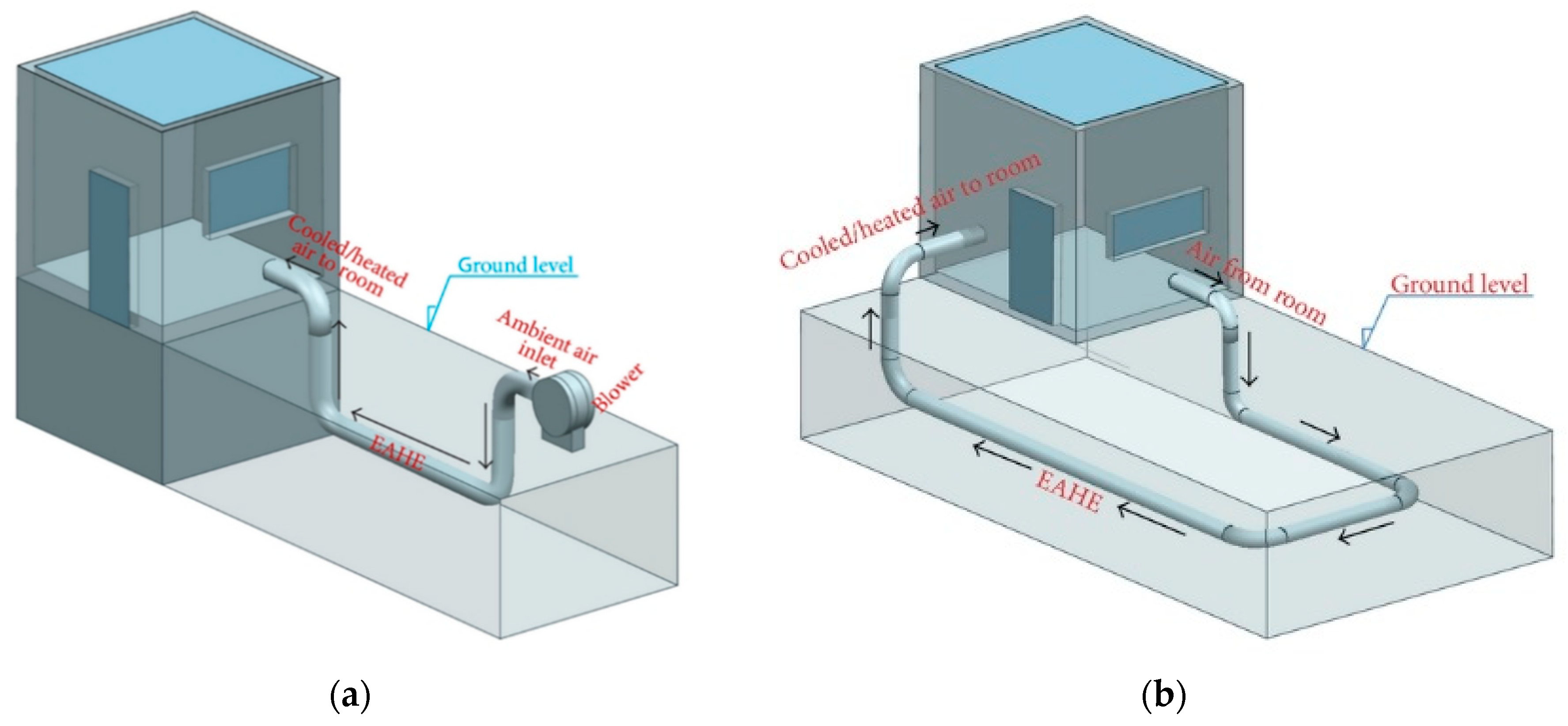
EAHE systems are divided into subgroups based on their configuration and design into open-loop and closed-loop EAHEs. Open loop EAHEs draw air directly from the atmosphere as shown in Figure 1a, while closed-loop EAHEs loop the air from a building until the desired temperature is achieved as shown in Figure 1b [12]. EAHEs can become a viable alternative to conventional air conditioning systems while giving a simplistic design and mitigating environmental concerns and costs at the same time [13]. The open loop system is preferred over closed loop as it provides the clean fresh air that circulates through pipes and meets the building cooling/heating requirements as compared to the closed loop where the same air is recirculated through the pipes [12].
EAHEs have been used for passive air conditioning, but they are impacted by several factors, such as weather, surface temperature, soil temperature and composition, and the geometry of the pipes [14]. Therefore, site selection for EAHEs is governed by the soil properties, including soil density, thermal diffusivity, conductivity, and the water and rock bed, and the process is complex [15].
The two performance indicators for EAHE are the temperature drop (temperature difference between the inlet and outlet air) and heat transfer rate. These two factors should be optimized using proper methodology/techniques to improve the performance of EAHE systems [16]. Several methodologies have been employed to investigate the performance of EAHE systems, summarized as follows.
A model incorporating projections of soil-temperature variations with time and depth was developed based on transient heat flow with certain assumptions. The model predictions had 85% to 90% accuracy as compared to the experimental data [17]. Another one-dimensional model incorporating convection diffusion with conduction processes was formulated for an air–earth–rock system. The system also considers humidity, it predicted temperature with 90% accuracy, and with a tolerance of 1.4 °C [18].
The relationship between burial depth, outlet temperature, Reynolds number, and the ratio of the pipe length to the diameter is addressed in [19]. It is indicated that the outlet temperature is inversely related to the pipe ratio (length to diameter ratio) and directly proportional to the Reynolds number and burial depth [19].
Convective heat transfer is estimated for large rectangular cross-sectional area EAHE systems. Computational Fluid Dynamics (CFD) simulations were used to train Artificial Neural Network (ANN) models [20]. Parametric studies were carried out and mathematical relationship between six design parameters and Average Nusselt numbers were established. It was revealed that surface temperature variation, duct outlet section size, and turbulence intensity of air had no effect on average Nusselt numbers. However, it was affected by duct length, inlet cross section area, the temperature difference between surface and inlet air, air velocity, and different operating modes [20].
Fuzzy logic controller is applied to optimize the power consumption in an EAHE system [21]. It was revealed that by using the fuzzy logic controller instead of an on–off controller less energy is consumed by the EAHE system [21]. Using Genetic algorithm, the EAHE system is evaluated and optimized for four parameters, i.e., air humidity, ambient air temperature, sub-soil temperature, and ground surface temperature [22].
With an increase in the length of the pipe, temperature drops between inlet air and outlet air increases but the rate of change of temperature decreases [23]. Similarly, after a certain length, the heat transfer remains the same with an increase in the length of the pipe, this phenomenon is termed as saturation length. With an increase in airflow, the saturation length also increases [24]. Pipe length is the most influential variable that affects the thermal performance of the EAHE system [25].
A low-velocity airflow provides more contact between the pipe and air hence increasing the heat transfer. An air velocity from 0.5 to 2.5 was considered for cooling performance of an EAHE system; where it was found that at the lowest flowing air velocity the temperature drop was maximum [26]. In an experimental study [27], three different velocities were considered for the pipe with a diameter of 0.1 m and length 19.2 m. It was observed that the maximum temperature drop of 12.9 °C occurs at 2 m/s and the minimum temperature drop occurs at 11.3 °C at 5 ms−1 [27].
The number of passes and geometrical configuration of pipes also impacts the EAHE performance. A numerical investigation of different geometrical configurations of pipes of an EAHE system shows that the thermal performance was enhanced by up to 115% and 73% for heating and cooling, respectively, by increasing the number of buried pipes covering the same area and accommodating the fixed mass flow rate [28]. The performance of an EAHE can be improved by using multiple-pipe configurations. A multiple-pipe configuration with a separation of 1.5 m and a depth of 3 m has better thermal performance than a single-pipe configuration [29].
In a simulation study of an EAHE system [30], three different parameters were simulated. The three parameters were inlet air temperature, ground temperature, and airflow rate in laboratory conditions. The highest heat transfer rate was observed at airflow of 0.07 kg s−1 and ground temperature of 23 °C. In addition, the highest temperature drop of 9.62 °C occurred at 0.07 kg s−1 and ground temperature of 23 °C [30].
The thermal performance of an EAHE system was simulated in the Energy Plus program (simulation software to model energy consumption in buildings) in [31]. It was concluded that the thermal performance depends up on the pipe depth and length. Results indicated that an EAHE module can reduce the cooling load by almost 50% [31]. The model in [32] studied in the hot, arid climatic conditions of Kuwait, analyzing the climatic impact. It was found that the EAHE system could not perform alone in these conditions but could be used and performed best in conjunction with a conventional air conditioning system [32]. A numerical simulating model [18] based on fluid dynamics and heat transfer conditions is modelled to predict the thermal behavior of EAHE. The model predicts that the temperature remains constant at 3 m depth. In addition, the model does the same computation, 45% faster, compared to other model [18]. The EAHE system causes a decrease of 8 °C in summer and an increase of 2 °C in winter. A Quasi mathematical model was developed in MATLAB using an energy balance equation in [33]. Air and soil temperatures were estimated using CFD. The parametric study for pipe length and pipe diameter for three different materials i.e., polyvinyl chloride (PVC), steel, and copper was reported to be the same [33].
1.1. Response Surface Method (RSM)
The Response Surface Method (RSM) was introduced by Box and Wilson for optimization of engineering problems [34]. It employs various approximate optimization techniques based on mathematical and statistical models. Through these techniques, a response that depends on various parameters is optimized [35]. RSM consists of two essential components i.e., Design of Experiment (DoE) and Regression Analysis. DoE is a systematic method that gives the design sample between input variables and the output response variable. Regression analysis estimates the response variable under the influence of independent variables [36]. The process of RSM is similar to that of experimental process [37]. First of all, the influencing factors are identified, and their response are measured at various levels. Secondly, through ANOVA (Analysis of Variance) the significant factors, individual effect, and interaction effect is determined. Lastly, using the regression equation the response is predicted for any unknown values of significant factors [37].
The Response Surface Method is based on the following steps [38]:
- Design experiment and measure responses at various levels of variables
- Develop and apply first and second response surfaces
- Determine parameters influencing the process for maximum and minimum responses
- Identify correlations between the variables through plots
- Develop a regression equation for significant parameters
The response surface is given as a function of independent and continuous variables by the following equation:
where n is the number of variables influencing the response function Y. It is rather important to establish a valid functional correlation between the response surface and variables.
Limited research outcomes have been reported in which a statistical optimization technique is used to identify the significant contribution of these parameters, optimize these significant parameters, and to predict the performance of EAHE systems on the basis of the contribution of these significant parameters.
In this paper statistical optimization methodology is used, in contrast to the previously prevalent simulation-based models and mathematical models used for parametric study of the influencing variables. A mathematical model is developed both for predicting sub-soil temperature using soil model and performance, i.e., temperature drop in flowing air and heat transfer of EAHE systems using the EAHE model. Parametric analysis is carried out using an EAHE mathematical model to determine the levels for the selected three parameters (length, diameter, and air velocity) for further optimization through the optimization technique Response Surface Method. This paper is structured in different sections. Section 1 introduces the concept of EAHE system and RSM and also summarizes previous literature on these topics. Section 2 outlines the materials and methodology used in this research. Section 3 explains and discusses the results of the study. Section 4 concludes the study with findings.
2. Materials and Methods
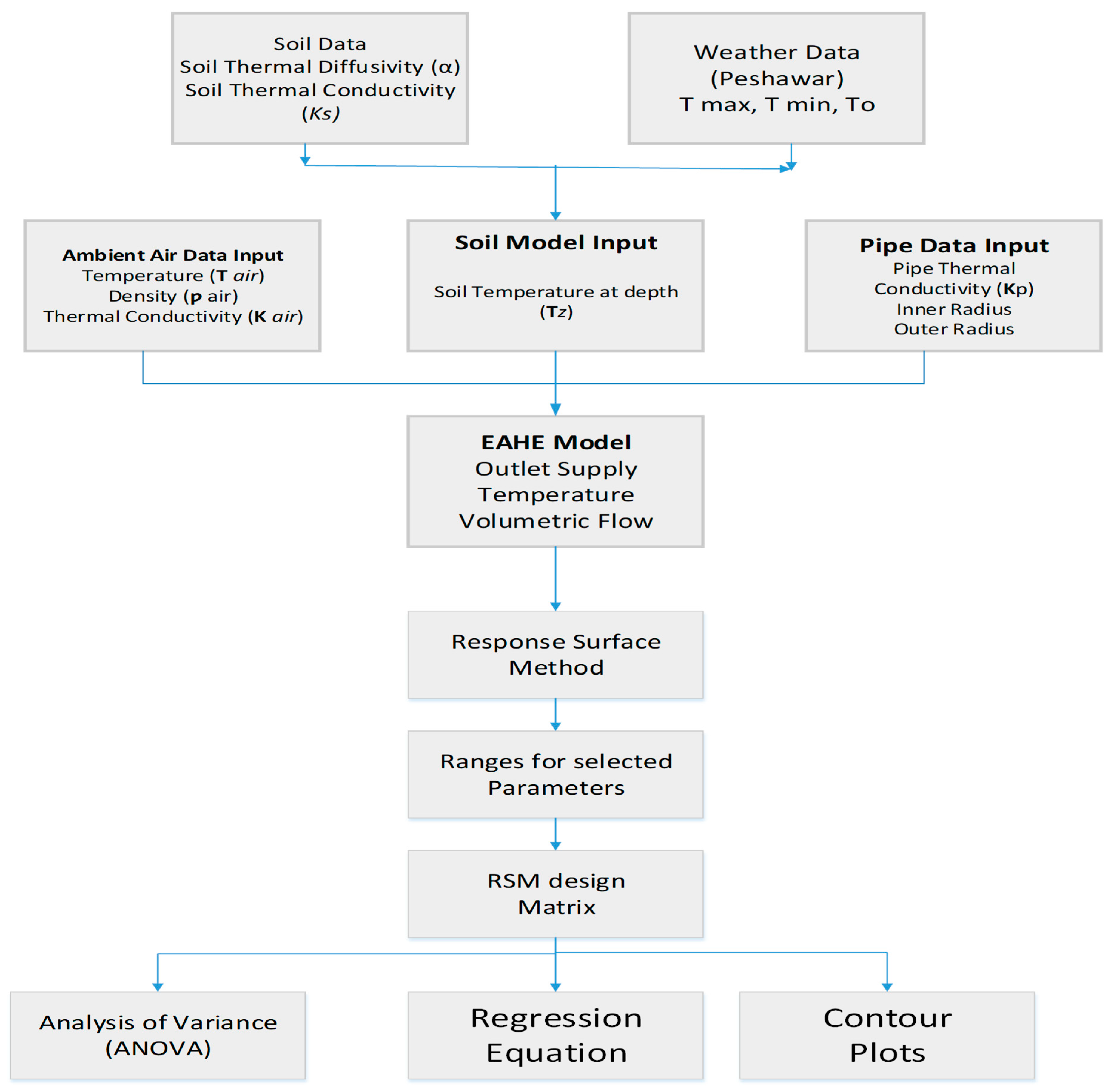
A new methodology is employed in this study shown in Figure 2. For this purpose, mathematical models are developed both for the soil and the EAHE is given in Section 2.1. Both the models are developed using heat transfer and energy balance governing equations. The models are experimentally validated in Section 3.2.
The soil model takes the thermal properties of soil and weather data as inputs. The soil characteristic properties are determined through the standard Proctor test conducted in Soil Lab [39]. The weather data was collected for three years from weather station in Peshawar City and is given in Section 2.2. The EAHE model takes pipe geometry and boundary conditions as inputs. The mathematical models are used to estimate the heat transfer and outlet temperatures of an EAHE model. For optimization of geometric parameters, a three-bedroom house was considered as the case study. The cooling load for each room is calculated using Hourly Analysis Program (HAP) software [40] and is outlined in Section 2.3. RSM is used to optimize the cooling load/heat transfer rate in Section 2.4.
2.1. Mathematical Models
The mathematical models were developed using heat transfer equations from the literature contribution by various researchers in this field [7,31,32,41]. To estimate the thermal performance indicators, which in this study are outlet temperature and heat transfer, the soil model and EAHE model were developed.
2.1.1. Soil Model
A soil model was developed to forecast the soil temperature at system depths using the heat conduction principle. When applied to a semi-infinite solid, the heat conduction principle [17] predicts the soil temperature T(t,z) at various times of year (t) and at different depths (z). The standard for ground temperature is assumed to be equal to the surface temperature in most cases [7,39].
The thermal diffusivity α is estimated by Equation (3) [42]:
2.1.2. Earth-To-Air Heat Exchanger Model
The EAHE model is based on the following assumptions:
- One dimensional heat transfer phenomena
- Homogeneous thermal properties of soil in the vicinity of the pipe
- Uniform pipe cross section
- Insignificant thermal effect of soil (i.e., soil not impacted by the presence of the EAHE with distance between the pipes equal to double the pipe radius)
A PVC pipe was used in the analysis. The pipe has a length (L) with an inner radius R1 and outer radius R2. The ambient air from the outside environment flows into the underground buried pipes. The pipes are buried at a known depth (z). The soil temperature is known, and the soil-layer radius is double the radius of the pipe. Equation (5) indicates the heat exchange occurring between air flowing through the pipe and the soil layer around the pipe as the ratio of the total temperature variation to the resistance to the heat flow between the higher and lower temperature regions [42].
The total thermal resistance is given by the following equation:
Equation (9) gives the Nusselt number for the total air flowing through a circular pipe [32].
where the friction (f) against the airflow for a smooth pipe can be estimated by Equation (10) [24].
The heat transfer occurring between the air and soil may be taken as the heat loss by the air to the pipe [32].
The temperature of air leaving at the outlet of the pipe is calculated by solving the above equation for the air temperature flowing through the pipe in the following three cases [32]. Firstly, if Tamb > T (t,z), then Equation (15) is used.
Tout = T (t,z) + eA.
If Tamb is equal to T (t,z), then Equation (16) is considered.
Tout = T (t,z).
If Tamb is less than T (t,z), then Equation (17) is employed.
where
Tout = T (t,z) − eA,
All of the above equations were generated in an excel sheet to calculate the outlet temperature.
2.2. Data Acquisition
The soil model requires the annual weather data, soil texture (soil composition), and moisture content in the soil as input data. The moisture content and soil composition are required to determine the soil’s thermal conductivity and diffusivity. For this purpose, weather data were acquired for Peshawar from the Metrological Data Centre for the years 2014–2016. The annual mean temperature calculated from the three years of data was 21.95 °C, and the annual mean amplitude variation was 6.23 °C.
Soil-texture and moisture-content were determined using the Proctor soil compaction test [43] in a soil lab at Peshawar. The moisture content and maximum dry density of the soil were determined for three different sites and at different depths through a soil Proctor test.
The Proctor soil compaction test is the process by which densification of soil is carried out by reducing air voids. The degree of compaction of a given soil is measured in terms of its dry density. The dry density is maximum at the optimum water content. The water content and the dry density are plotted to obtain the maximum dry density and the optimum water content as per Equation (19) [44]. The list of equipment used in the test is listed in Table 1.
where is soil dry density, w = water content, M = Mass of the soil, V is the volume of soil.
2.3. Building Configuration
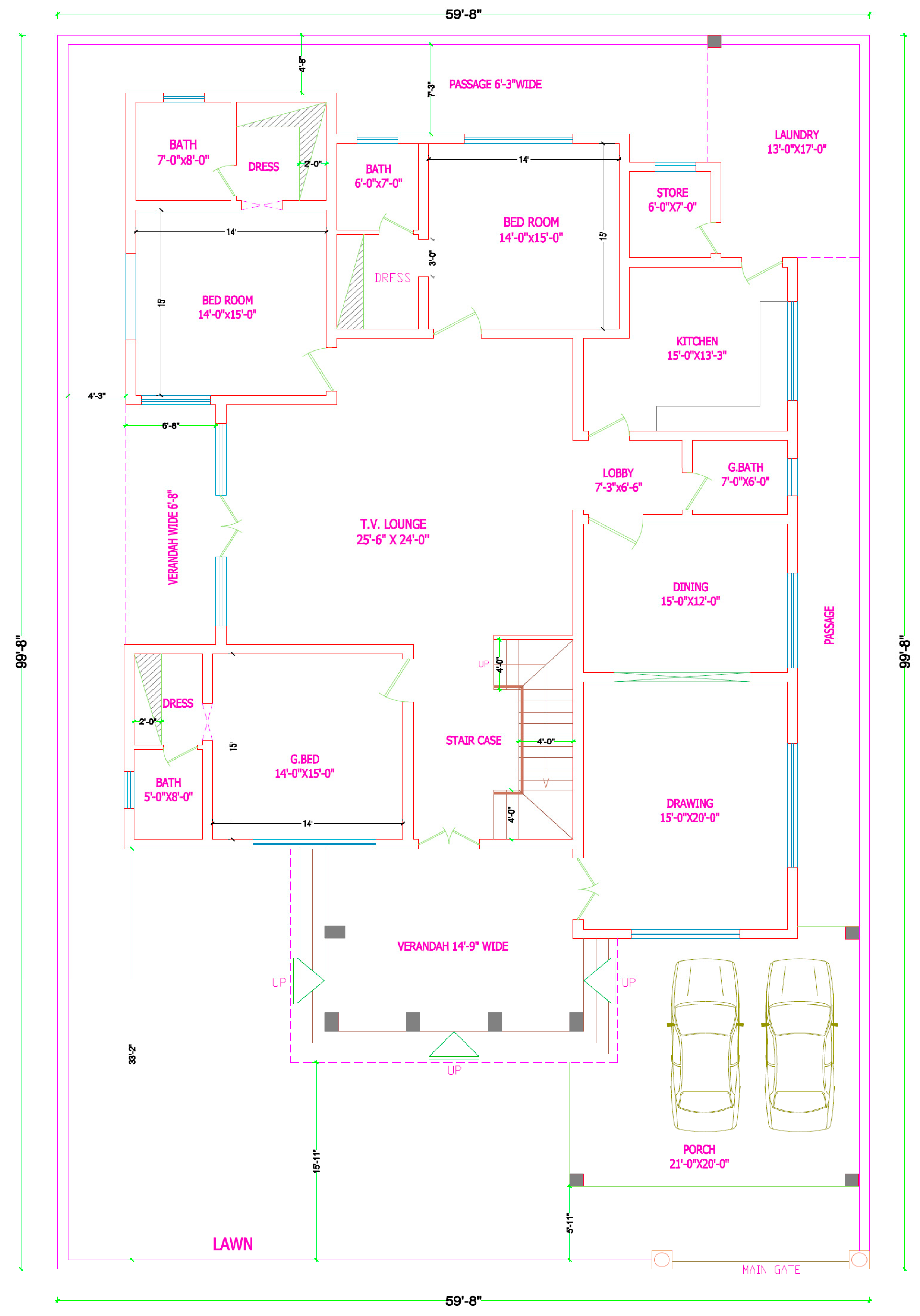
A house with three bedrooms was selected as a case study for which the cooling load was calculated using HAP software. Figure 3 represents the schematic drawing of the three-bedroom house. The description of the building is given in Table 2. The house is located in Peshawar, Pakistan. The building faces south, with GPS coordinates of 34.0151°N, 71.5249°E. The walls are single block bricks with a thickness of 10.16 cm (0.1016 m) and 1.27 cm (0.0127 m) on both sides of the wall. Each room has an area of 19.509 m2 and ceiling height of 10 ft. Each room has three lights of 7 W, a 70 W fan and some other electrical equipment contributing minor load. On average, medium level activity is selected with two occupants for each room. The rooms are provided with a single door, a window, and a ventilator, which contributes to the air infiltration. For an unconditioned space, the minimum and maximum temperatures are 23 and 44 °C. The weather data was gathered from Karachi Metrological Data Centre for Peshawar city. The total cooling load, calculated using HAP software [40], for the three rooms was 8.4 kW/h (2.9 kW/h for each room).
2.4. Response Surface Method (RSM) for Optimization
Response Surface Method (RSM) is a statistical technique for determining the significance of various parameters in a problem for response optimization on a surface of interest, as detailed in Section 1.1. A response surface design was created in Minitab software (A Statistical Tool) [45], which was used to create and analyze Response Surface Design by employing RSM. A central composite design was used for three continuous factors i.e., length, diameter, and air velocity. Each factor has three levels that makes 20 runs in total in the design matrix. Furthermore, full factorial design with face center design was selected inside the central composite design. The runs were randomized by selecting the randomized option. After designing the design matrix, the response surface design was analyzed using full quadratic analysis with confidence level of 95%.
3. Results
3.1. Proctor Soil Compaction Result
The mean soil density of the samples was 1900 kg/m3, and the average moisture content was 9.11%. These soil properties were used as input to determine the thermal conductivity and diffusivity in the soil-model equations. The thermal properties were used to predict the temperature of the sub-soil surface at any depth and time of the year.
3.2. Model Validation
Two separate experiments (from the literature) based on disparate climatic and soil conditions were used for model validation [46,47]. The input parameters used in the model are given in Table 1. The first experiment [46] was carried out in Ajmer, India, on 8 April 2009, and the model predicted the actual outcomes of the experiments with more than 95% confidence. The climatic condition for Peshawar, Pakistan, and Ajmer, India have similar climatic conditions [48]. Both the cities have local steppe climate. The climate is considered to be hot semi-arid climate (type “BSh”) according to the Köppen–Geiger climate classification [49]. Similarly, the proposed model predicts the experimental results of [46,47] shown in Table 3 and Table 4 with more than 90% confidence. Thus, keeping in view the accuracy of these results, the proposed model can be used in the design and performance analysis of EAHEs.
3.3. Parametric Analysis Using EAHE Validated Model
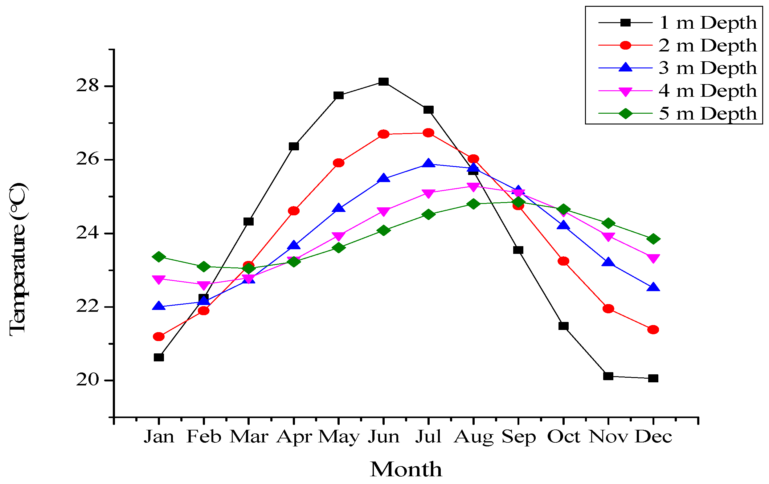
Using the above validated EAHE model, the parametric analysis was carried out to identify the levels of the selected three parameters i.e., length, diameter, and air velocity. The soil model was used to determine the temperature at different installation depths. Table 5 gives an idea of the values of the input parameters for the soil model. These input parameters are calculated from weather data and soil compaction test as explained above in Section 2. The annual amplitude variation for Peshawar city is 6.23 °C, its mean annual temperature is 21.95 °C and the thermal conductivity of the soil is 1.45 W/(m. °C).
Figure 4 shows that there is lower temperature variation at higher depths. The graphs flatten at higher depths because the annual temperature variations are minimal. There are comfortable temperatures between 20 and 26 °C at an installation depth of 3 m. Consequently, an installation depth of 3 m was selected for the EAHE system to achieve a maximum temperature of 26 °C and minimum of 20 °C. The month of July was specifically targeted for this study because it is the hottest month with a mean temperature of 39 °C and the highest recorded temperature for the year at 44 °C.
3.4. Influence of Various Parameters on EAHE System
The proposed EAHE model was used to estimate the impacts of various parameters on the outlet temperature and its contribution to the cooling load. For this purpose, three key parameters were investigated for their impact on the temperature: the length, air velocity, and diameter. With the base value fixed for each parameter, the impact was assessed with gradual increments of the other variables. These values are presented in Table 6.
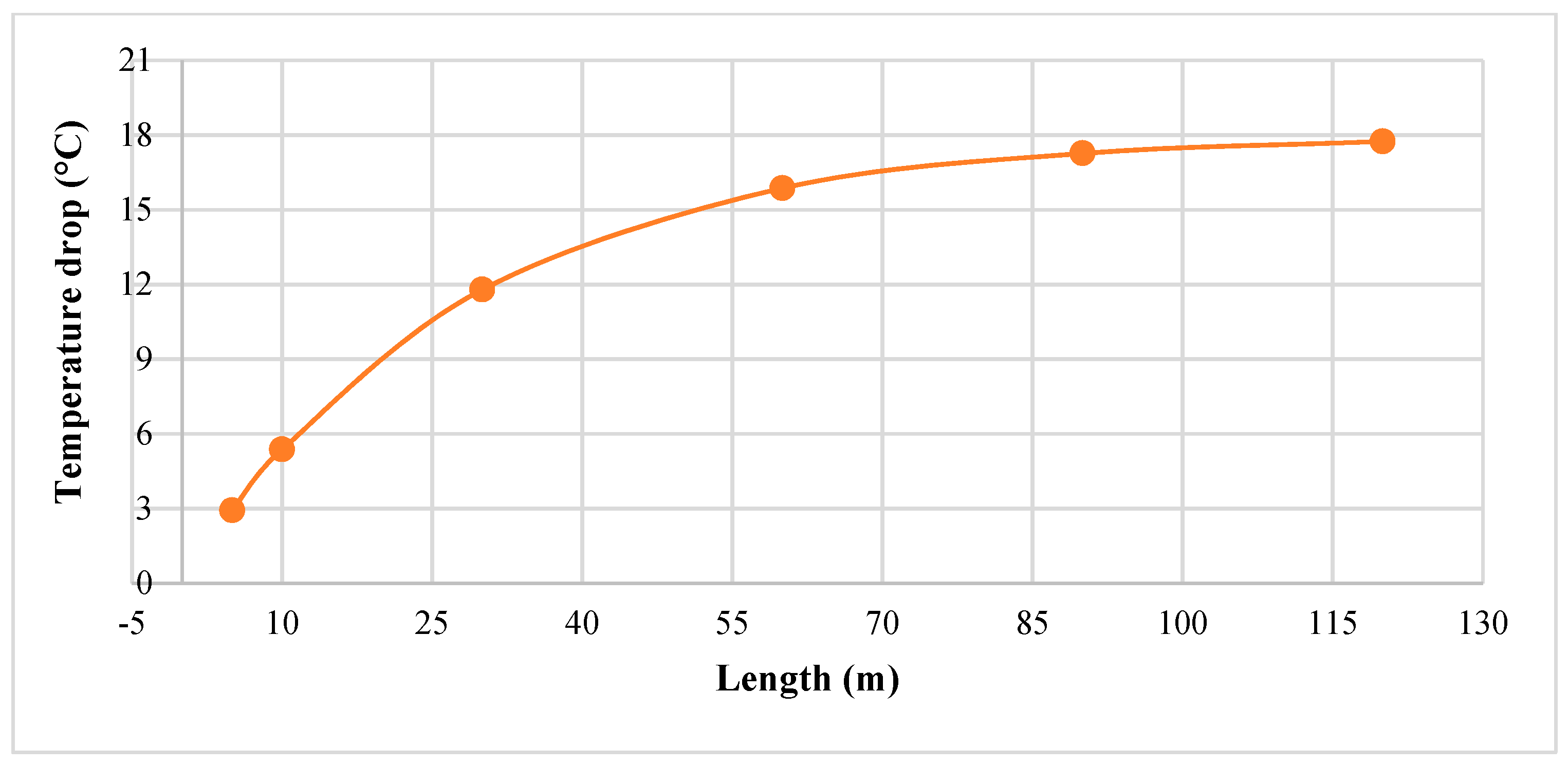
3.4.1. Influence of Length
The impact of length on the temperature difference between inlet and outlet (temperature drop) is shown in Figure 5, where a direct relationship is observed. As length of the pipe increases, the air has more time in contact with the pipe and thus with the lower temperatures of the soil. In addition, when keeping the velocity and flow rate of the air constant, impact of the length dissipates after 60 m. The greater the temperature drop across the EAHE system, the more heat transfer will occur, and as a result more cooling load will be compensated.
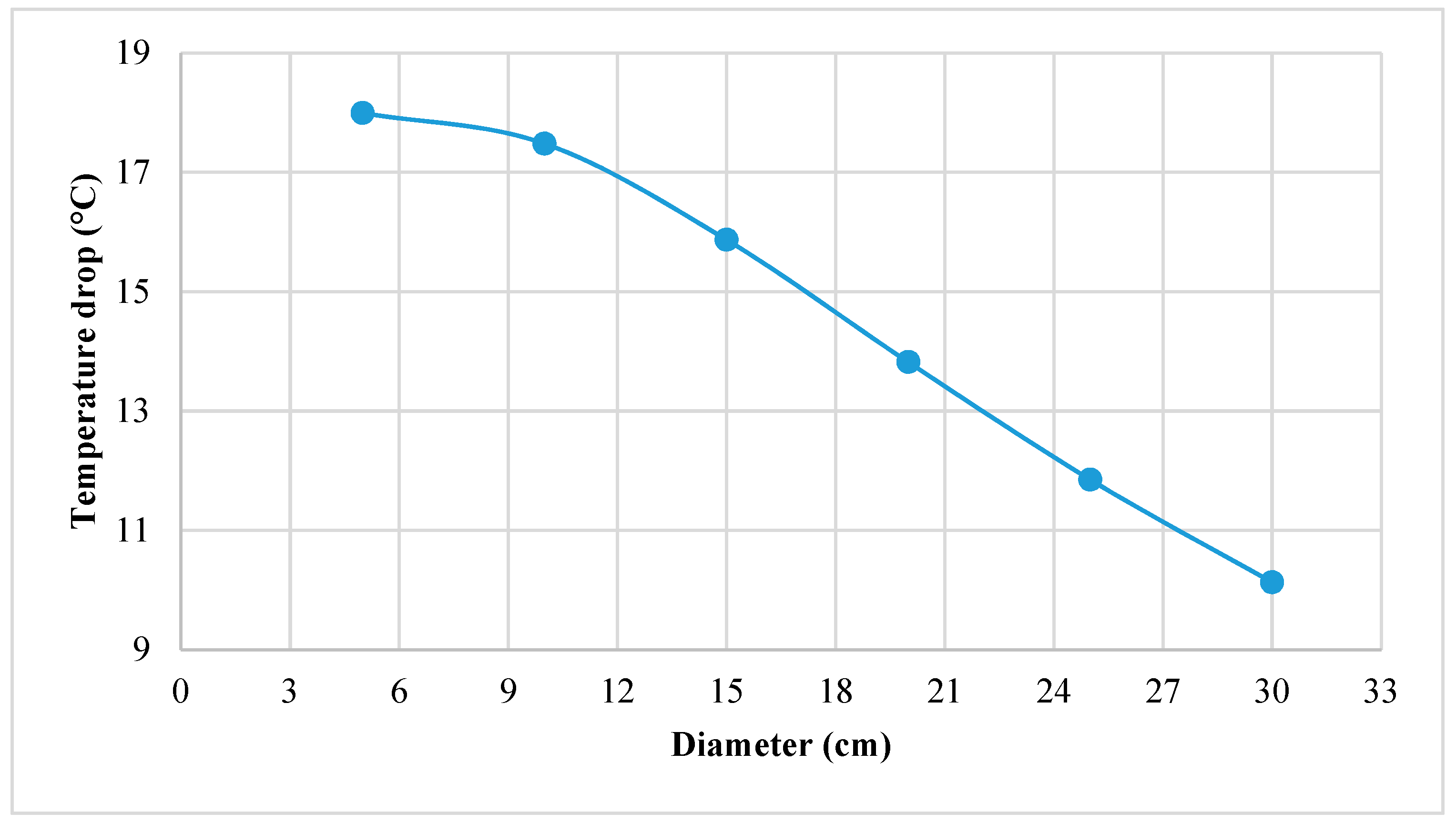
3.4.2. Influence of Diameter
Impact of the pipe diameter on the temperature difference between inlet and outlet (temperature drop) is presented in Figure 6, which shows a decrease in the rate of the temperature drop with increasing diameter. One reason for this is that the primary source of heat exchange is convective heat transfer, meaning that by increasing the diameter while keeping the same air flow, the contact surface of air will decrease. In addition, the effective range of the diameter of the pipe is between 10 and 30 cm. As heat transfer is a product of temperature drop and volumetric air flow, by decreasing diameter below 10 cm the temperature drop will be increase but the heat transfer rate will decrease due to lesser volumetric flow and increased pressure drop. By increasing diameter above 30 cm the effectiveness of the temperature drop decreases, resulting in a decrease in overall heat transfer.
3.4.3. Influence of Air Velocity
The impact of air velocity on the temperature drop of the inlet air is shown in Figure 7, which shows a negative relation. As the air velocity across the pipe decreases, the temperature difference between inlet and outlet (temperature drop) decreases. It is because the air is in contact with the surface of the pipe for less time when moving with higher velocity. The effective range of air velocity for the optimum temperature drop across the pipes is between 2 and 6 m/s when keeping the pressure change in check. The parametric analysis helped in the determination of the working ranges of the length, velocity, and diameter for the EAHE system. These ranges were used in the response surface design matrix.
The above results indicate how the different geometric and control parameters affect the temperature drop. The length is directly proportional to the temperature drop at the outlet of the pipe. It also suggests that the temperature drop at the outlet is inversely proportional to the diameter and air velocity. The above influence gave the preliminary idea to the designer about the effective ranges for better performance of the EAHE system.
3.5. RSM Results (Sensitivity Analysis)
The RSM design matrix was given 20 runs for the three levels of each parameter, and is given in Table 7. Each of these runs gave a set of values for the parameters through the proposed model. After the selection of the quadratic order for the data analysis, an Analysis of Variance (ANOVA) was conducted for the parameters with the response function (Delta Q). Delta Q was estimated using EAHE mathematical model.
The results of the ANOVA are presented in Table 8, which indicates the overall significance of the model and establishes its adequacy with a p-value less than the confidence interval value of 0.5.
The F value is the ratio between two means squares. If the F value is larger, the null hypothesis can be rejected and there will be significant variation in the group mean. The RSM analysis gave F values of 99.74, 407.52, and 67.14, for the length, air velocity, and diameter, respectively. The larger F values for the diameter compared to the length and air velocity indicate a greater contribution of the diameter to the system performance than the other two parameters. It is also evident from the table that there is a significant interaction between the three factors with p-values less than 0.05 for all interactions, while the F-value for the length–diameter interaction is greater than that of the other two interactions.
The model summary of the ANOVA in Table 9 shows 98.13% and 74.46% agreement between R-sq (adj) and R-sq (pred), respectively, which validates the model.
Since the model was proven adequate, the response function may be estimated with the regression equation as follows:
Delta Q = 1630 − 16.6 L − 13,729 D − 188 Av − 0.30 L2 + 4175 D2 − 14.31 Av2 + 295.81 L × D + 4.76 L × Av + 1634 D × Av.
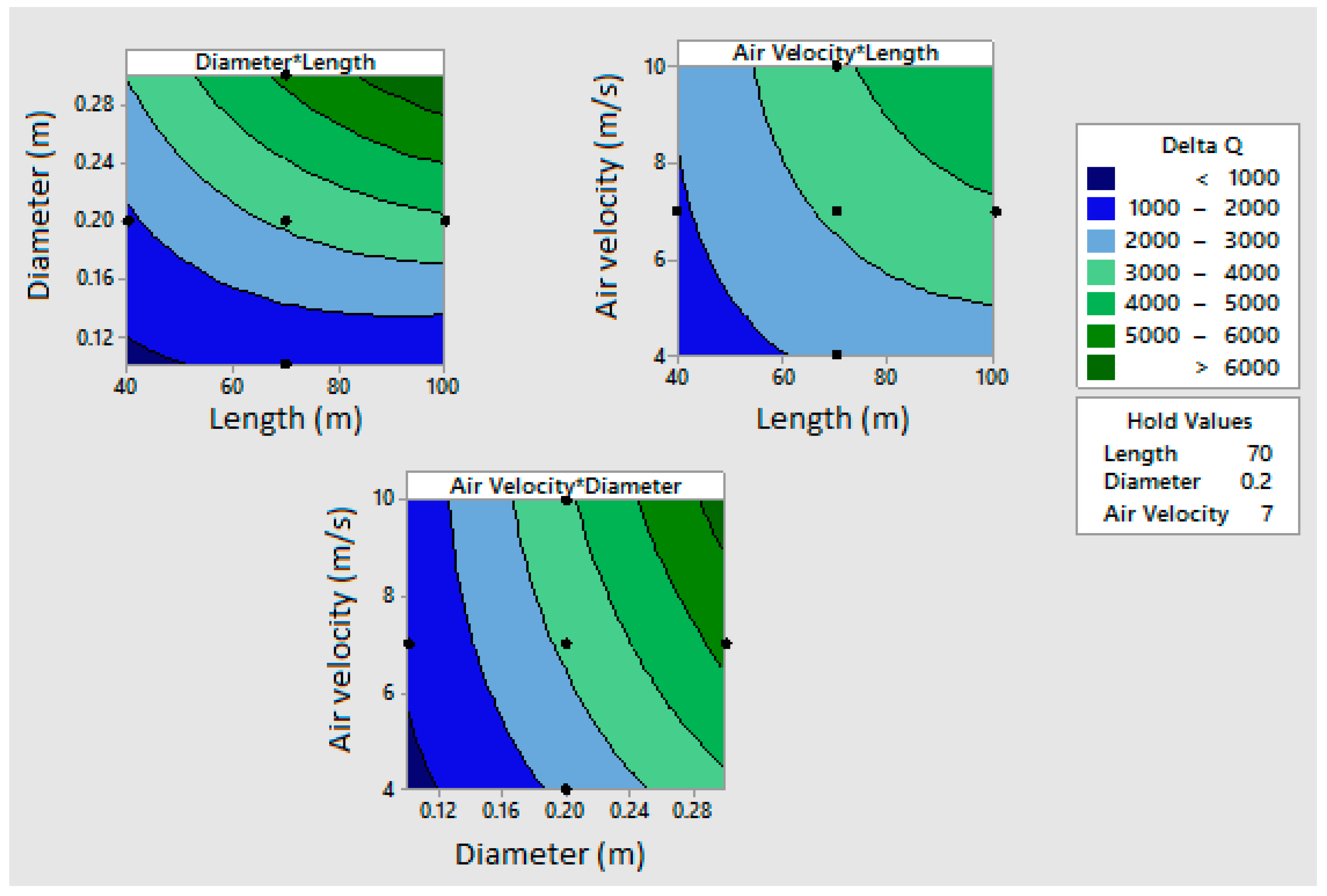
Figure 8 shows contour plots for the three parameters’ interaction while keeping the third parameter constant. The cooling load calculated for a single room is approximately 3 kW/h. The contour plot is rising ridge shaped which means as the color gets darker it represents the extreme values. The dark blue represents lowest extreme while the dark green represents the highest extreme. In the contour plot between Diameter × Length while keeping the air velocity at 7 ms−1, the maximum load cooling that can be compensated in the range of 5–6 KW for diameter values ranges between 0.24 and 0.28 m and length ranges between 70 and 100 m. The minimum load that can be compensated is between 1 and 2 kW for length values ranging from 40 to 100 m, whereas diameter ranges from 0.10 to 0.21 m. The load of a single room is 3 kW, which is represented by border line between the light blue and light green region. It can be compensated for length ranges between 40 and 100 m whereas the diameter ranges from 0.18 to 0.30 m. Any value between these ranges can be selected to pay off single room load trading off between the length and diameter values.
Similarly, in the contour plot between air velocity and length while keeping the value of diameter at 0.2 m, the maximum cooling load that can be compensated ranges between 4 and 5 kW. It can be achieved for length and air velocity values ranges between 78 and100 m and 7.8 and 10 ms−1 respectively. The minimum load that can be paid off is between 2 and 3 kW for length ranges between 40 and 62 m for air velocity that lies between 4 and 8.2 ms−1. The border line between the light green and light blue region represents the load of a single room. Selecting any point on this line gives values for length and air velocity respectively.
In the case of the contour plot between air velocity and diameter while keeping the length at 70 m, the border line between the light blue and light green regions represents the cooling load of a single room. Any point on this line corresponds to its air velocity and diameter values respectively. The maximum load that can be compensated at constant length of 70 m is 5 to 6 kW. This load is achieved for air velocity and diameter values ranges between 0.26 and 0.30 m respectively.
The contour plot gives the idea of different configurations of influencing variables i.e., length, diameter, and air velocity available for the same cooling ranges. On the other hand, the regression equation estimates the cooling load for any specific configuration of the influencing variables.
4. Discussion
A new approach for optimization of EAHE was successfully developed using statistical modeling in contrast to the simulation-based models prevalent in the literature. Three influencing variables, length, diameter, and air velocity, were studied and optimized using the statistical optimization technique called RSM. A house in Peshawar city of Pakistan was used as a case study. The results gathered using mathematical models and optimization techniques led to the following findings.
- The soil model predicts that temperature varies between 20 and 26 °C at a depth of 3 m. Therefore, the optimal depth to install the EAHE system is 3 m or more to achieve an outlet temperature between 20 and 26 °C for the weather and soil conditions of Peshawar.
- The effectiveness of the design parameters was determined. The effective length for the earth-to-air heat exchanger, for which a significant amount of temperature drop occurs, lies between 20 and 70 m. The effective diameter that significantly influences the temperature drop lies between 0.1 and 0.3 m, and for air velocity the range is 3 to 7 m/s.
- RSM indicates that all the three design parameters have a significant effect on the heat transfer rate (cooling load) and the model used is significant, as indicated by ANOVA (see Table 6). Diameter is the most significant contributor to the cooling load with the largest F-value compared to length and air velocity. Similarly, the length and diameter have the largest interaction effect on the cooling load, having the largest F-value compared to other interaction effects i.e., length and air velocity and diameter and air velocity. Regression Equation (19) can be used to predict the heat transfer rate (cooling load) using any value of the significant parameters, which are length, diameter, and air velocity.
- In addition, from the contour plot (Figure 8) between air velocity and diameter for holding the length at 50–70 m, the 3 KW cooling load, which is the cooling load for a single room, can be achieved with between 0.18 and 0.25 m in diameter and air velocity ranging from 5 to 7 m/s.
The RSM optimization technique gives different ranges for the cooling load with different alternatives. It would help the designers in decision making to select the cheapest alternative in terms of pipe material, excavation cost, and installation cost. The soil model predicts the underground temperature knowing the underground temperature profile, and optimal depth where the temperature lies between the ranges of thermal comfort can be selected. Resultantly, it helps in minimizing excavation costs to dig up the land for installation of pipes. Moreover, as shown in the contour plots, the same amount of cooling load wattage can be compensated using a range for each parameter. Regression Equation (19) estimates the cooling load for any value of the influencing parameter as an input. In contrast to using complex simulation tools, using the proposed approach, the designers and manufactures can use any statistical tool to design the EAHE systems efficiently and effectively. The major disadvantage of this approach is that it does not accommodate the condensation factor inside the pipes, which will be incorporated into a future model. In previous studies the influencing variables were discussed but their significant impact on the performance of EAHEs was not proven statistically; it is proven in this study.
Before reaching the current developed method in the manuscript, extensive literature reviews were carried out. Previously, high-end software like CFD and other fluid analysis and building management software were used for analysis and optimization. This software is expensive, requires high-computing-power computers, and expertise in operating the software. Current methodology uses simple heat transfer and energy governing equations to design, analyze, and then using statistical techniques the parameters influencing the performance of system are optimized. This approach can easily be implemented using simple statistical tools. This approach is useful as it does not need high computing power computers and expertise in this field.
The EAHE system is clean and green as it does not contribute to greenhouse gases emissions. The working fluid in this technology is air rather than refrigerants. It has negligible maintenance costs as it uses just a simple blower fan, and the expected system life depends upon the pipe’s life. It can be used stand-alone or can be integrated with conventional HVAC systems to minimize the cost associated with maintaining thermal comfort inside the building. The limitations of EAHE system is its initial capital cost and the availability of land to install this system.
Moreover, the methodology is not case specific. It takes soil data and weather data as an input for any building load. The contour plot (Figure 8) provided different alternatives. For example, for a cooling load of 3 kW, each point on a border line between light blue and light green gives a different configuration of pipe parameters and air flow. Each of these points are different alternatives. Using this approach, the contour plots gives an idea of different configuration of influencing variables i.e., length, diameter, and air velocity. The regression equation generated as a result of this approach predicts the cooling load for any selected alternative based on a tradeoff between different alternatives. The cost associated with different configurations of pipe parameters and blower power consumption for same cooling load can be estimated based on the information provided by the contour plots. The alternatives can be evaluated and decisions shall be made based on the cost benefit analysis of each of these alternatives.
5. Conclusions
It can be concluded that the models developed can be used to design, analyze, and optimize the earth-to-air heat exchanger thermal performance. The optimum ranges for influencing parameters were identified. In addition, the model can be used and applied to other soil and climatic conditions using the same approach developed in this study. Using the approach in this study, it is evident that the earth-to-air heat exchanger can be used in buildings to reduce the conventional air-conditioning load of the devices. Additionally, multiple pipes should be used to fulfill the cooling demand of the whole building, as a single pipe can meet the demand only of a single room with these optimum ranges of length, diameter, and air velocity. This model is equally applicable for optimal designing of earth-to-air heat exchangers for different soil and weather conditions. If these three inputs (soil data, weather data, and building cooling load) are available, the same methodology can be applied to optimally design the EAHE system for a specific building cooling load under specific soil and weather conditions.
Author Contributions
This work is primarily based on MS thesis of Engr M., supervised by T.A., S.A., N.M., A.A., M.S. and A.B. helped in methodology and results sections and contributed equally to the paper.
Funding
The paper was funded by United States Agency for International Development through US Pakistan Center for Advanced Studies in Energy (USPCAS-E), UET Peshawar Pakistan.
Acknowledgments
The authors would like to thank USPCAS-E, UET Peshawar, Pakistan for their extended support in making this research work possible.
Conflicts of Interest
The authors declare no conflict of interest.
Nomenclature
| T(t:z) | Temperature (°C) of soil (days, depth) | Rconvec | Thermal resistivity caused by convection (m2 °C/W) |
| Tmean | Annual average temperature °C | Air Mass flow rate (kg/s) | |
| Tamp | Annual temperature variation (amplitude) | R3 | Soil annulus radius = pipe total radius |
| Ca | Specific heat of air (J/kg K) | ΔT | Total drop in temperature |
| Kair | Thermal conductivity of air (W/m °C) | R1 | Pipe’s inner radius (m) |
| F | Friction coefficient of pipe | Rt | Thermal resistivity (m2 °C/W) |
| Kp | Thermal conductivity of pipe (W/m °C) | Re | Reynold number |
| Tamb | Air temperature (Ambient) °C | R soil | Thermal resistivity caused by soil annulus (m2 °C/W) |
| Hc | Convective heat transfer coefficient (W/m °C) | Ut | Pipe’s overall thermal conductivity (W/m °C) |
| Ks | Thermal conductivity of soil (W/m °C) | Pr | Prandtl Number |
| Z | Depth of the system (m) | W | Moisture content of the soil (%) |
| T | Time | Tf | Fluid temperature in the pipe (°C) |
| A | Soil’s thermal diffusivity | Ts | Soil temperature (°C) |
| Rpipe | Pipe’s radius | Cs | Specific heat of soil (J/kg K) |
| R2 | Pipe’s total radius (m) | ρs | Density of soil (kg/m3) |
| to | Maximum recorded temperature of the year, Phase constant | M | Total mass of the soil (Kg) |
| Ks | Thermal Conductivity of soil (W/m °C) | ANN | Artificial Neural Network |
| V | Volume of the soil (m3) | EAHE | Earth-to-air heat exchanger |
| HAP | Hourly Analysis Program |
References
- Kåberger, T. Progress of renewable electricity replacing fossil fuels. Glob. Energy Int. Dev. Coop. Organ. 2018, 1, 48–52. [Google Scholar]
- Sohail, M.; Qureshi, M.U.D. Energy-Efficient Buildings in Pakistan. Sci. J. COMSATS—Sci. Vis. 2011, 16, 27–38. [Google Scholar]
- Ra, M.M.; Rehman, S.; Asia, S. National energy scenario of Pakistan—Current status, future alternatives, and institutional infrastructure: An overview. Renew. Sustain. Energy Rev. 2017, 69, 156–167. [Google Scholar]
- Aized, T.; Mehmood, S.; Anwar, Z. Building energy consumption analysis, energy saving measurements and verification by applying HAP software. Pakistan J. Eng. Appl. Sci. 2017, 21, 1–10. [Google Scholar]
- Ahmad, K.; Rafique, A.F.; Badshah, S. Energy Efficient Residential Buildings in Pakistan. Energy Environ. 2014, 25, 991–1002. [Google Scholar] [CrossRef]
- Singh, R.; Sawhney, R.L.; Lazarus, I.J.; Kishore, V.V.N. Recent advancements in earth air tunnel heat exchanger ( EATHE ) system for indoor thermal comfort application: A review. Renew. Sustain. Energy Rev. 2018, 82, 2162–2185. [Google Scholar] [CrossRef]
- Ozgener, L. A review on the experimental and analytical analysis of earth to air heat exchanger (EAHE) systems in Turkey. Renew. Sustain. Energy Rev. 2011, 15, 4483–4490. [Google Scholar] [CrossRef]
- Sobti, J.; Singh, S.K. Earth-air heat exchanger as a green retrofit for Chandīgarh—A critical review. Geotherm. Energy 2015, 3, 14. [Google Scholar] [CrossRef]
- Soni, S.K. Heating/Cooling Techniques used in Green Buildings: A Review. Int. J. Emerg. Tech. 2019, 10, 1–8. [Google Scholar]
- Park, K.; Kim, S. Utilising Unused Energy Resources for Sustainable Heating and Cooling System in Buildings: A Case Study of Geothermal Energy and Water Sources in a University. Energies 2018, 11, 1836. [Google Scholar] [CrossRef]
- Baglivo, C.; D’Agostino, D.; Congedo, P.M. Design of a Ventilation System Coupled with a Horizontal Air-Ground Heat Exchanger (HAGHE) for a Residential Building in a Warm Climate. Energies 2018, 11, 2122. [Google Scholar] [CrossRef]
- Bisoniya, T.S.; Kumar, A.; Baredar, P. Study on Calculation Models of Earth-Air Heat Exchanger Systems. J. Energy 2014, 2014, 1–15. [Google Scholar] [CrossRef] [Green Version]
- Pfafferott, J. Evaluation of earth-to-air heat exchangers with a standardised method to calculate energy efficiency. Energy Build. 2003, 35, 971–983. [Google Scholar] [CrossRef]
- Kumar, R.; Kaushik, S.C.; Garg, S.N. Heating and cooling potential of an earth-to-air heat exchanger using artificial neural network. Renew. Energy 2006, 31, 1139–1155. [Google Scholar] [CrossRef]
- Chen, Y.; Shi, M.; Li, X. Experimental investigation on heat, moisture and salt transfer in soil. Int. Commun. Heat Mass Transf. 2006, 33, 1122–1129. [Google Scholar] [CrossRef]
- Agrawal, K.K.; Bhardwaj, M.; Misra, R.; Agrawal, G.D.; Bansal, V. Optimization of operating parameters of earth air tunnel heat exchanger for space cooling: Taguchi method approach. Geotherm. Energy 2018, 6, 1–17. [Google Scholar] [CrossRef]
- Ozgener, O.; Ozgener, L.; Tester, J.W. A practical approach to predict soil temperature variations for geothermal (ground) heat exchangers applications. Int. J. Heat Mass Transf. 2013, 62, 473–480. [Google Scholar] [CrossRef]
- Su, H.; Liu, X.B.; Ji, L.; Mu, J.Y. A numerical model of a deeply buried air-earth-tunnel heat exchanger. Energy Build. 2012, 48, 233–239. [Google Scholar] [CrossRef]
- Sehli, A.; Hasni, A.; Tamali, M. The potential of earth-air heat exchangers for low energy cooling of buildings in South Algeria. Energy Procedia 2012, 18, 496–506. [Google Scholar] [CrossRef]
- Zhang, J.; Haghighat, F. Development of Artificial Neural Network based heat convection algorithm for thermal simulation of large rectangular cross-sectional area Earth-to-Air Heat Exchangers. Energy Build. 2010, 42, 435–440. [Google Scholar] [CrossRef]
- Diaz, S.E.; Sierra, J.M.T.; Herrera, J.A. The use of earth–air heat exchanger and fuzzy logic control can reduce energy consumption and environmental concerns even more. Energy Build. 2013, 65, 458–463. [Google Scholar] [CrossRef]
- Kumar, R.; Sinha, A.R.; Singh, B.K.; Modhukalya, U. A design optimization tool of earth-to-air heat exchanger using a genetic algorithm. Renew. Energy 2008, 33, 2282–2288. [Google Scholar] [CrossRef]
- Derbel, H.B.J.; Kanoun, O. Investigation of the ground thermal potential in tunisia focused towards heating and cooling applications. Appl. Therm. Eng. 2010, 30, 1091–1100. [Google Scholar] [CrossRef]
- Benhammou, M.; Draoui, B. Parametric study on thermal performance of earth-to-air heat exchanger used for cooling of buildings. Renew. Sustain. Energy Rev. 2015, 44, 348–355. [Google Scholar] [CrossRef]
- Ahmed, S.F.; Amanullah, M.T.O.; Khan, M.M.K.; Rasul, M.G.; Hassan, N.M.S. Parametric study on thermal performance of horizontal earth pipe cooling system in summer. Energy Convers. Manag. 2016, 114, 324–327. [Google Scholar] [CrossRef]
- Niu, F.; Yu, Y.; Yu, D.; Li, H. Heat and mass transfer performance analysis and cooling capacity prediction of earth to air heat exchanger. Appl. Energy 2015, 137, 211–221. [Google Scholar] [CrossRef]
- Bisoniya, T.S.; Kumar, A.; Baredar, P. Parametric Analysis of Earth-Air Heat Exchanger System Based on CFD Modelling. Int. J. Power Renew. Energy Syst. 2014, 1, 36–46. [Google Scholar]
- Kepes Rodrigues, M.; da Silva Brum, R.; Vaz, J.; Oliveira Rocha, L.A.; Domingues dos Santos, E.; Isoldi, L.A. Numerical investigation about the improvement of the thermal potential of an Earth-Air Heat Exchanger (EAHE) employing the Constructal Design method. Renew. Energy 2015, 80, 538–551. [Google Scholar] [CrossRef]
- De Jesus Freire, A.; Coelho Alexandre, J.L.; Bruno Silva, V.; Dinis Couto, N.; Rouboa, A. Compact buried pipes system analysis for indoor air conditioning. Appl. Therm. Eng. 2013, 51, 1124–1134. [Google Scholar] [CrossRef]
- Yusof, T.M.; Ibrahim, H.; Azmi, W.H.; Rejab, M.R.M. Thermal analysis of earth-to-air heat exchanger using laboratory simulator. Appl. Therm. Eng. 2018, 134, 130–140. [Google Scholar] [CrossRef]
- Lee, K.H.; Strand, R.K. The cooling and heating potential of an earth tube system in buildings. Energy Build. 2008, 40, 486–494. [Google Scholar] [CrossRef]
- Al-Ajmi, F.; Loveday, D.L.; Hanby, V.I. The cooling potential of earth-air heat exchangers for domestic buildings in a desert climate. Build. Environ. 2006, 41, 235–244. [Google Scholar] [CrossRef]
- Serageldin, A.A.; Abdelrahman, A.K.; Ookawara, S. Earth-Air Heat Exchanger thermal performance in Egyptian conditions: Experimental results, mathematical model, and Computational Fluid Dynamics simulation. Energy Convers. Manag. 2016, 122, 25–38. [Google Scholar] [CrossRef]
- Myers, C.M.A.C.R.H.; Montgomery, D.C. Response Surface Methodology: Process and Product Optimization Using Designed Experiments, 4th ed.; Wiley: Hoboken, NJ, USA, 2016. [Google Scholar]
- Gao, H. Medium optimization for the production of avermectin B1a by Streptomyces avermitilis 14-12A using response surface methodology. Bioresour. Technol. 2009, 100, 4012–4016. [Google Scholar] [CrossRef] [PubMed]
- Wang, S.; Xiao, J.; Wang, J.; Jian, G.; Wen, J.; Zhang, Z. Application of response surface method and multi-objective genetic algorithm to configuration optimization of Shell-and-tube heat exchanger with fold helical baffles. Appl. Therm. Eng. 2018, 129, 512–520. [Google Scholar] [CrossRef]
- Jones, R. Design and Analysis of Experiments (fifth edition), Douglas Montgomery, John Wiley and Sons, 2001, 684 pages, £33.95. Qual. Reliab. Eng. Int. 2002, 18, 163. [Google Scholar] [CrossRef]
- Hou, T.H.; Su, C.H.; Liu, W.L. Parameters optimization of a nano-particle wet milling process using the Taguchi method, response surface method and genetic algorithm. Powder Technol. 2007, 173, 153–162. [Google Scholar] [CrossRef]
- Gurtug, Y.; Sridharan, A.; İkizler, S.B. Simplified Method to Predict Compaction Curves and Characteristics of Soils. Iran. J. Sci. Technol. Trans. Civ. Eng. 2018, 42, 207–216. [Google Scholar] [CrossRef]
- Carrier United Technologies. Hourly Analysis Program. 2018. Available online: https://www.carrier.com/commercial/en/us/software/hvac-system-design/hourly-analysis-program/ (accessed on 12 December 2018).
- Gouda, S.G.A. Using of Geothermal Energy in Heating and Cooling of Agricultural Structures. Master’s Thesis, Moshtohor Benha University, Banha, Egypt, 2010. [Google Scholar]
- ASHRAE. Handbook Heating, Ventilating, and Air-Conditioning System and Equipement; The American Society of Heating, Refrigerating and Air Conditioning Engineers, Inc.: Atlanta, GA, USA, 2012. [Google Scholar]
- Das, B.M. Soil Mechanics Laboratory Manual; Oxford University Press: Oxford, UK, 2002; pp. 35–44. [Google Scholar]
- Gopal Mishra. Proctor Soil Compaction Test—Procedures, Tools and Results. The Constructor Civil Engineering Home. Available online: https://theconstructor.org/geotechnical/compaction-test-soil-proctors-test/3152/ (accessed on 22 March 2019).
- Kent State University. Minitab. 2019. Available online: https://libguides.library.kent.edu/statconsulting (accessed on 26 March 2019).
- Bansal, V.; Misra, R.; Agrawal, G.D.; Mathur, J. Performance analysis of earth-pipe-air heat exchanger for summer cooling. Energy Build. 2010, 42, 645–648. [Google Scholar] [CrossRef]
- Shingari, B.K.; Singh, A.; Sapra, K.L. Earth Tube Heat Exchanger. Poult. Int. 1995, 34, 92–97. [Google Scholar]
- Merkel, A. Climate-Data.org. AM Online Projects. 2019. Available online: https://en.climate-data.org (accessed on 28 May 2019).
- Kottek, M.; Grieser, J.; Beck, C.; Rudolf, B.; Rubel, F. World Map of the Köppen-Geiger climate classification updated. Meteorol. Zeitschrift 2006, 15, 259–263. [Google Scholar] [CrossRef]
Figure 1.
(a) Open loop earth to air heat exchanger. (b) Closed loop earth to air heat exchanger.

Figure 2.
Methodology flow chart.

Figure 3.
Residential building drawing.

Figure 4.
Variation of annual temperature at different depths.

Figure 5.
Influence of length on the temperature drop.

Figure 6.
Influence of diameter on the temperature drop.

Figure 7.
Influence of air speed on the temperature drop.

Figure 8.
Contour plots for sensible cooling load with respect to the influencing parameters.


Table 1.
List of equipment used in the Proctor compaction test.
| List of Equipment | ||
|---|---|---|
| 1. Compaction mold | 2. Rammer | 3. Detachable Base Plate |
| 4. Collar | 5. IS Sieve | 6. Oven |
| 7. Oven | 8. Desiccator | 7. Mixing tools, spoons, towel |
Table 2.
Building configuration.
| Building Description | Three Bed Room House |
|---|---|
| Location | Peshawar |
| Building Face | South |
| Coordinates | 34.0151°N, 71.5249°E |
| Walls | Single Brick 5′(4′ + 0.5″ + 0.5″) |
| General Bed Room Size | 14 × 15 (210 sq ft) |
| Maximum Temperature | 44 °C |
| Minimum Temperature | 23 °C |
Table 3.
Model validation with experimental results [46].
Table 3.
Model validation with experimental results [46].
| EAHE Parameters | Tsoil = 26.7 °C | Length = 23.4 m | Diameter = 0.15 m | |
|---|---|---|---|---|
| Ambient Temp. | Air Velocity | Outlet Temp. (Bansal et al.) | Outlet Temp. (Proposed Model) | Relative Error (%) |
| 42.2 | 5 | 34.2 | 35.5 | 3.82 |
| 42.3 | 4 | 33.5 | 34.8 | 3.68 |
| 42.5 | 3 | 33.1 | 33.9 | 2.41 |
| 43.4 | 2 | 33.1 | 33.2 | 0.30 |
Table 4.
Model validation with experimental results [47].
Table 4.
Model validation with experimental results [47].
| EAHE Parameters | Tsoil = 20 °C | Diameter = 0.20 m | Length = 13 m | |
|---|---|---|---|---|
| Ambient Temp. | Air Velocity | Outlet Temp. (Shingari et al.) | Outlet Temp. (Proposed Model) | Relative Error (%) |
| 39.6 | 10.5 | 35.4 | 37.51 | 5.96 |
| 37.5 | 4.5 | 33.5 | 34.07 | 1.70 |
| 38.6 | 1.3 | 31.1 | 32.18 | 3.47 |
| 33.6 | 0.5 | 30.3 | 28.13 | 7.16 |
Table 5.
Soil model input parameters.
| Parameters | Tamp °C | Tmean °C | Depth (z) Meter (m) | Phase Constant Days (to) | Thermal Conductivity W/(m. °C) |
|---|---|---|---|---|---|
| Values | 6.23 | 21.95 | 1 to 5 | 139 | 1.45 |
Table 6.
Earth-to-air heat exchange (EAHE) model parameters.
| Parameters | Soil Temp. (°C) | Soil Depth (m) | Length (m) | Diameter (m) | Ambient Temp. (°C) | Air Velocity (m/s) |
|---|---|---|---|---|---|---|
| Base value | 26 | 3 | 60 | 0.15 | 44 | 5 |
Table 7.
Response Design Matrix.
| Length (m) | Diameter (m) | Air Velocity (m/s) | Delta Q (W) | Length (m) | Diameter (m) | Air Velocity (m/s) | Delta Q (W) |
|---|---|---|---|---|---|---|---|
| 70 | 0.2 | 7 | 3148.43 | 70 | 0.2 | 7 | 3148.43 |
| 70 | 0.2 | 4 | 1995.48 | 100 | 0.2 | 7 | 3616.05 |
| 100 | 0.3 | 4 | 4706.65 | 70 | 0.1 | 7 | 968.46 |
| 70 | 0.2 | 7 | 3148.43 | 70 | 0.3 | 7 | 5377.38 |
| 40 | 0.1 | 10 | 794.56 | 70 | 0.2 | 7 | 3148.43 |
| 70 | 0.2 | 7 | 3148.43 | 70 | 0.2 | 7 | 3148.43 |
| 100 | 0.3 | 10 | 8655.35 | 100 | 0.1 | 4 | 569.23 |
| 40 | 0.3 | 4 | 2261.09 | 40 | 0.3 | 10 | 3342.36 |
| 100 | 0.1 | 10 | 1404.35 | 40 | 0.1 | 4 | 520.60 |
| 40 | 0.2 | 7 | 2096.02 | 70 | 0.2 | 10 | 4008.95 |
Table 8.
Analysis of Variance (ANOVA) results.
| Source | Degree of Freedom | Adj Sum of Square | Adj Mean Square | F Value | p Value |
|---|---|---|---|---|---|
| Model | 09 | 67,138,561 | 7,459,841 | 74.34 | 0.00 |
| Linear | 03 | 56,863,992 | 18,954,663 | 190.46 | 0.00 |
| Length (L) | 01 | 9,874,399 | 9,874,399 | 99.74 | 0.00 |
| Diameter (D) | 01 | 40,343,241 | 40,343,241 | 407.52 | 0.00 |
| Air velocity (Av) | 01 | 6,646,353 | 6,646,353 | 67.14 | 0.00 |
| Square | 03 | 582,017 | 194,006 | 1.96 | 0.18 |
| Length × length | 01 | 208,174 | 208,174 | 2.10 | 0.18 |
| Diameter × diameter | 01 | 4793 | 4793 | 0.05 | 0.83 |
| Air velocity × air velocity | 01 | 45,731 | 45,731 | 0.46 | 0.51 |
| Two-way interaction | 03 | 9,692,551 | 3,230,850 | 31.94 | 0.00 |
| Diameter × length | 01 | 6,301,474 | 6,301,476 | 64.15 | 0.00 |
| Air velocity × length | 01 | 1,469,401 | 1,469,403 | 15.14 | 0.00 |
| Air velocity × diameter | 01 | 1,921,674 | 1,921,674 | 18.91 | 0.00 |
| Error | 10 | 989,978 | 98,992 | ||
| Lack of fit | 05 | 989,976 | 197,997 | ||
| Pure-error | 05 | ||||
| Total | 19 | 68,128,531 |
Table 9.
Model summary.
| S | R-Square | R-Square (adj) | R-Square (pred) |
|---|---|---|---|
| 313.63 | 99.14% | 98.23% | 74.46% |
© 2019 by the authors. Licensee MDPI, Basel, Switzerland. This article is an open access article distributed under the terms and conditions of the Creative Commons Attribution (CC BY) license (http://creativecommons.org/licenses/by/4.0/).
Share and Cite
MDPI and ACS Style
Maoz; Ali, S.; Muhammad, N.; Amin, A.; Sohaib, M.; Basit, A.; Ahmad, T. Parametric Optimization of Earth to Air Heat Exchanger Using Response Surface Method. Sustainability 2019, 11, 3186. https://doi.org/10.3390/su11113186
AMA Style
Maoz, Ali S, Muhammad N, Amin A, Sohaib M, Basit A, Ahmad T. Parametric Optimization of Earth to Air Heat Exchanger Using Response Surface Method. Sustainability. 2019; 11(11):3186. https://doi.org/10.3390/su11113186
Chicago/Turabian StyleMaoz, Saddam Ali, Noor Muhammad, Ahmad Amin, Mohammad Sohaib, Abdul Basit, and Tanvir Ahmad. 2019. "Parametric Optimization of Earth to Air Heat Exchanger Using Response Surface Method" Sustainability 11, no. 11: 3186. https://doi.org/10.3390/su11113186
Note that from the first issue of 2016, this journal uses article numbers instead of page numbers. See further details here.