Application of Wavelet-Based Maximum Likelihood Estimator in Measuring Market Risk for Fossil Fuel

Abstract

Energy commodity prices are inherently volatile, since they are determined by the volatile global demand and supply of fossil fuel extractions, which in the long-run will affect the observed climate patterns. Measuring the risk associated with energy price changes, therefore, ultimately provides us with an important tool to study the economic drivers of climate changes. This study examines the potential use of long-memory estimation methods in capturing such risk. In particular, we are interested in investigating the energy markets’ efficiency at the aggregated level, using a novel wavelet-based maximum likelihood estimator (waveMLE). We first compare the performance of various conventional estimators with this new method. Our simulated results show that waveMLE in general outperforms these previously well-established estimators. Additionally, we document that while energy returns realizations follow a white-noise and are generally independent, volatility processes exhibits a certain degree of long-range dependence.

1. Introduction

The price quoted for an asset reflects the present value of a future stream of expected earnings. In an efficient market, any re-evaluation of the asset price must therefore immediately reflect unforeseen changes in those earnings. Conventional asset pricing theories show that the magnitude and frequency of such changes, whenever they appear, can be used as a measure of risk. Market imperfections cause prices to reflect information slowly, and sometimes the response to new information is dragged over a long period. This well-established empirical regularity, known as the long-range dependence of price observations, serves as the main theme of this paper.

Evidence of this phenomenon is most often illustrated by the slow hyperbolic decay rate of the autocorrelation function of empirical time series in the physical sciences. Similarly, it is widely documented that the evolution of the risk of financial assets’ returns constitutes a long-memory stochastic process. To be specific, this type of process is defined with a real number H and a constant $C$ such that the process’s autocorrelation is $\mathsf{\rho }\left(l\right)={\mathrm{Cl}}^{2\mathrm{H}-2}$ as the lag parameter $\mathrm{l}\to \infty$. We show later that the parameter $H$ is known as the Hurst exponent, named after the hydrologist Hurst who first analyzed the presence and measurement of long-memory behavior in stochastic processes [1]. In the following Section, we provide a theoretical background for studying the long-memory of volatility processes. Section 3 then demonstrates a plethora of well-established and robust methodologies aimed to detect and estimate the degree of long-memory characterized by the level of the Hurst exponent $H$. In Section 4, we demonstrate the performance of these methods using simulated data and show that the wavelet-based maximum likelihood estimator, originally formulated by [2], generally outperforms several other methods in most of the simulated experiments and is arguably inferior to none. The application of the wavelet estimator on actual energy price time series is the topic of Section 5, where we find support for long-memory in the spot returns of major global fossil fuels. Section 6 provides concluding remarks, the implications of our study, and qualifications for our results.

2. Related Literature

2.1. Long-Memory and Market Efficiency

In financial markets, analyses of long-range dependence of returns are known to yield mixed evidence and the implications of these studies create a focal point for intensive debate. This is because the existence of long-memory generally indicates predictability of future returns based on past returns, which violates the basic assumption of one of the most widely supported ideas in the history of economics, the efficient market hypothesis (EMH). The EMH, which was independently developed by [3,4], in its strongest form, assumes that the changes of stock price follow a random walk. The intuition (or seemingly counter-intuition) is that when all available information and/or all expectation is fully reflected in prices, one cannot forecast the price changes by simply looking at past prices. This implies that any informational advantage, even the smallest, is instantaneously exposed and incorporated into market prices when the investors possessing it try to make profit from it. In this “ideal” scenario, prices follow a martingale, which is the cornerstone of traditional asset pricing and derivative pricing models. Therefore, violation of this condition would undermine the foundation of these models. For example, conventional linear models of returns such as the classic capital asset pricing model (CAPM) will encounter numerous problems should price changes not be random. Furthermore, if long-range dependence exists, implications from economics disciplines that are sensitive to investment horizons such as optimal consumption decision and portfolio management would be affected [5]. The seminal paper by [4], as well as the earlier work by [6,7], are among the first to document the stylized fact of low or insignificant serial correlation in returns of stocks and commodities. Other studies, however, suggest a substantial negative serial correlation, indicating markets tend to reverse themselves over long periods (see, e.g., [8]).)

In contrast to the mixed evidence for long-memory returns, such behavior is widely observed to be a “stylized fact” of the risk of financial volatility. Among the early advocates of this vein of thought are [9,10], while [5] opposed it. Long-memory is also related to theories of trade and business cycles. Widely documented long-range dependence displayed by time series from multiple economics contexts has inspired [11] to relate this phenomenon to the prophecy made by Joseph (a biblical reference from the Old Testament), who predicted that Egypt was to have seven years of prosperity followed by seven years of famine. Hence the fanciful yet perhaps aptly termed “Joseph effect” often accompanies the more popularly known “Hurst effect” in the long-memory modelling literature.

A number of academics consider the Hurst exponent, or the “index of dependence”, as a component of the so-called chaos theory (see, e.g., [12]). Based on this theory, an alternative to the EMH, the fractal market hypothesis (FMH), is proposed. This hypothesis casts doubt on the “ideally” uniform and simultaneous interpretation of information reflected in prices (which is embraced by EMH); instead, it assumes that traders may decipher information in different ways and at different times. If investors are influenced by events from the past, price changes are not entirely unpredictable. The FMH also assumes non-normal, leptokurtic distribution of price changes, and price decreasing faster than it increases, all of which are empirically true. Intuitively, if stock prices follow a random walk/Brownian motion under the general assumption of the EMH, then its logarithmic difference (or the financial returns) should be normally distributed. Yet in practice, the overwhelming evidence of heavy tailed returns distribution suggests stock prices do exhibit dependence to some extent, thus invalidating the EMH. Perhaps one of the strongest criticisms to date against the classic EMH is presented in the work of [13].

Additionally, it should be noted that modern financial economists generally reject the notion of a “static” sense of market efficiency and adopt an adaptive, evolutionary perspective instead. Indeed, it would be unreasonable to assume that efficiency can be maintained consistently, as evident by numerous incidents related to inefficiencies such as value stocks and small firms yielding returns higher than market average or the various crashes over the years implying severely mispriced assets. More relevant to our study, it is the stylized clustering behavior of stock returns and the predictability of the financial data generating process due to its inherent long-memory that may have shaken the universal foundation of market efficiency.

These observations have led to a new consensus that relates efficiency to economic development. In particular, as economies gradually evolve from an under-developed to a sophisticated state, we would expect to see a corresponding movement towards efficiency of financial markets in the form of correctly priced assets. Obviously, this is not a static process, nor is it a short-term one. Adopting this approach, [14] use Hurst index estimates to show that different stages of emerging economies correspond to increasing levels of efficiency and exhibit different degrees of long-memory. The principle of this idea is consistent with [15], who support a “self-correction” viewpoint in which arbitrageurs attracted by mispriced assets would eventually enforce efficiency. Thus, in a way, inefficiency takes an indispensable role in maintaining efficiency itself. Along the same line, in his seminal article, [16] attempted to reconcile the assumption of market rationality with the various psychological aspects of the documented irrationality among investors and introduced another alternative to the EMH, the adaptive market hypothesis (AMH). In essence, the AMH is a synthetic compromise between two seemingly conflicting schools of thinking: the EMH and behavioral finance. The latter advocates ubiquitous behavioral biases (e.g., over-confidence, over-reaction, or herding) that could lead to distortions of utility optimizing decisions that form the basis of the former. In a sense, this means that to the AMH, extreme market movements such as crashes are nothing more than conditions facilitating a ‘natural selection’ process that casts out investors that could not adapt to the ever-changing market environment. As such, compared to the EMH, the AMH allows for “[…] considerably more complex market dynamics, with cycles as well as trends, and panics, manias, bubbles, crashes, and other phenomena that are routinely witnessed in natural market ecologies” [16] (p. 24).

Compared with the extensive literature on long-memory of conventional economic and financial time series and commodities markets, investigation of long-memory models with respect to fossil fuel markets is only newly developed. Ref. [17] is the first to document evidence of long-memory in absolute return, squared return, and conditional volatility of spot and futures returns for oil and refined products even in the presence of structural breaks. Subsequently, [18,19,20], among many others, confirm the existence of long-memory with GARCH-type models, and that models that account for structural breaks, parameter instability, and long-memory provide the best conditional volatility forecasts. Using modified rescaled range analysis and three local Whittle methods, [21] find that long-range dependence is only weakly exhibited by returns but strongly exhibited in volatilities of energy futures prices with different maturities. Recently, [22,23] incorporated Markov switching dynamics and semi-parametric approaches to GARCH frameworks to deliver improved out-of-sample oil prices and returns forecast performance. Our paper adds to this growing literature with the introduction of a wavelet-based estimator of long-memory, which will be discussed in Section 3.

2.2. The Hurst Index

The so-called ‘self-similarity parameter’ that is associated with long-memory process has a rich history. A British hydrologist named Edwin Hurst (1880–1978) was credited with the formation of this concept. A more formal definition is provided by [24] for both discrete-time and continuous-time stochastic processes. Here we only restate the definition in the continuous context: consider a stochastic process $\left\{X\left(t\right)\right\}(0\le t<\infty )$. It is said to be self-similar if the two processes, $\left\{X\left(at\right)\right\}$ and $\left\{a^{H}X\left(t\right)\right\}$, have identical finite-dimensional distribution for all $a > 0$. The parameter $a$ can be thought of as a “scaling” parameter so that the latter process is actually a scaled version of the former. Analogous to the notion of time series stationarity, there exists a weaker form of self-similarity when these processes have equal mean and covariance structure, which we refer to as second-order self-similar [25]. What does the Hurst exponent H imply? To be more specific, provided that the above condition holds when $0 < H < 1$, we have a self-similar process. In the special case of $1/2 < H < 1$, for a (weakly) stationary process, the second-order self-similarity also implies long-range dependence among present and distant past values of that process, a feature commonly referred to as “long-memory”.

Another definition of a broad long-memory class can be found in [26], which states that such process is well-defined if its autocorrelation function

$$\rho \left(l\right)=Cov\left(X_i,X_{i+l}\right)/Var\left(X_i\right)$$

(1)

is not summable and satisfies ${{\displaystyle \sum }}_{l=0}^{\infty }\rho \left(l\right)=\infty$. In this context, we assume that $\left\{Xt\right\}$ is a weakly stationary discrete time series. This implies a slowly decaying autocorrelation function, i.e., $\rho \left(l\right) \sim C\left|l\right|{}_{\alpha } \mathrm{when} \left|l\right| \to \infty$. This is the basic property of all processes belonging to the long-memory class, where C is a constant and 0 < α < 1 is a parameter representing the decay rate. (We will show later that in general α = 2 − 2H.) In this case the decay is said to follow a “power law”. Larger H implies stronger long-range dependence or more persistent impact of past events on present events. Conventional statistical inferences of processes exhibiting this feature can be dramatically altered. As [24] pointed out, for a process with finite variance and/or summable covariance such as an AR(1) process, the standard deviation of its mean is asymptotically proportional to $n^{1/2}$. This is a crucial condition for traditional statistical inferences to be meaningful. However, with long-range dependence introduced by a slow decaying $\rho \left(l\right)$, the same standard deviation is proportional to $n^{-\alpha /2}$, thus affecting all test statistics, as well as the confidence intervals for the estimate of the sample mean. The long-memory processes are contrasted with the short-memory class, which exhibits summable and exponential decaying co-variances (which was also termed short-range dependence or weak dependence). Ref. [5] made a clear distinction between these two classes, asserting that the short-memory behavior is characterized by the fact that “[…] the maximal dependence between events at any two dates becomes trivially small as the time span between those two dates increases” (p. 1281). In other words, the rate at which dependence decays is very high for processes exhibiting short-run dependence. Here we are only interested in what this means in an empirical financial context.

As discussed earlier, [1] was the first to propose a method to detect and estimate the widely observed and naturally occurring empirical long-term dependence in the form of the “rescaled range” statistic, denoted as $R/S\left(n\right)$ (where $n$ represents the sample size). Assuming that the process generating the empirical data is long-range dependent, this method aims to infer the Hurst exponent $H$ as implied by the relationship $E\left[R/S\left(n\right)\right] \sim C{n}^H$ when $n \to \infty$ and the finite positive constant $C$ is independent of $n$. This empirical law is referred to as the “Hurst effect”.

The parameter $H$ typically takes on a value in the interval $\left[0, 1\right]$ and if observations are generated from a short-range dependent process then $H = 0.5$. In this case the process is said to be “self-determining”. As there is no long-range dependence, the time series generated by such a process cannot be forecast from past information. This is analogous to the case when stock prices follow a Brownian motion, with discrete realizations following a random walk model. When $0 < H < 0.5$ we have an anti-persistent process, where past and present observations are negatively correlated. This means the behavior of subsequent observations contradicts that of previous observations, resulting in a tendency to revert towards the mean value. Such time series exhibit the phenomenon known as “mean-reversion” in financial literature. The tendency becomes stronger as H approaches zero. When $0.5 < H < 1$, which was the case of the annual Nile river flow time series in Hurst’s original paper, we have a long-memory process. Variations of this type of time series are too large to be explained by a pure random walk. Such processes exhibit a trending behavior, which could be interrupted by discontinuities. As shown above, one typical time series generated by such a process is known as a fractionally integrated series, with the ‘fractional’ degree of integration $d = H - 0.5$. Generally, the interpretation of $H$ and $d$ with regards to the nature of long-memory is summarized in

Table 1. Categorizing stochastic processes based on their long-memory property.

Hurst Exponent	Fractional Difference Parameter	Behavior of the Process
H ≤ 0	d ≤ −1/2	Non stationary
0 < H < 1/2	−1/2 < d < 0	Anti-persistent, mean-reversing
H = 1/2	d = 0	Random, Brownian motion
1/2 < H < 1	0 < d < 1/2	Long-range dependence
H ≥ 1	d ≥ 1/2	Non stationary

.

When tasked with estimating the optimal water storage level for the construction of reservoirs along the Nile, the rescaled range statistic indicated a high degree of persistence of the annual Nile river’s overflow, with a Hurst index of 0.91. Application and generalization of this method were popularized by [27], who were also among the first to study long-range dependence in financial time series. Equity risk exhibits a Hurst exponent estimated to be greater than 0.5, typically being 0.7 [13]. It would be interesting then to reconcile the trending behavior of stock returns implied by Hurst exponent estimates and the trend-detecting techniques which form the basis of so-called “technical analysis”. As it turns out, using a trading rule designed for capitalizing on the trending behavior of stock price during certain periods, [28] documented greater trading profit associated with a higher long-memory parameter at all the periods studied. On the other hand, this author also observed lower profits at times when the market exhibits mean-reversion behavior. Intuitively, technical trading strategies seeking to follow possible market ‘trends’ is expected to have some sort of correlation with the Hurst index, which is a measure of such trending behavior.

3. Methods for Estimating Long-Memory in Financial Time Series

3.1. Conventional Methods

A well-established technique for estimating the Hurst exponent is based on a statistic known as the “rescaled range over standard deviation” or “R/S” statistic. This statistic was first introduced in 1951 by the hydrologist H. E. Hurst who observed long range dependence in the dynamics of the Nile river’s annual water level to determine the long-term storage capacity crucial for the construction of irrigation reservoirs. Since then, robust empirical evidence of long-range dependence in time series has been extensively documented in various disciplines, particularly from physical science studies, where studied time series exhibit some kind of trending behavior (e.g., the circumferences of tree trunks, levels of rainfall, fluctuations in air temperature, oceanic movements, and volcanic activities, etc.). Among the first to use re-scaled range analysis to examine this behavior in common stock returns is the renowned econometrician B. Mandelbrot, who also coined the term Hurst exponent in recognition of Hurst. Refs [12,29] radically refined the R/S statistic. In particular, they advocate its robustness in detecting as well as estimating long-range dependence even for non-Gaussian processes with extreme degrees of skewness and kurtosis. Furthermore, this method’s superiority over traditional approaches such as spectral analysis or variance ratios in detecting long-memory was also presented in this body of research.

However, as [5] pointed out, the refinements were not able to distinguish the effects of short-range and long-range dependence. To compensate for this weakness, he proposed a new modified R/S framework. His findings indicate that the dependence structure documented in previous studies are mostly short-ranged, corresponding to high frequency autocorrelation or heteroskedasticity. There are two important implications for us from [5]: (i) empirical inferences of long-range behavior must be carefully drawn, preferably by accounting for dependence at higher frequencies, and (ii) in such cases, conventional models of short-range dependence model (such as AR(1) or random walk models) might be adequate. On the other hand, as implied in a counterargument raised by [30], we should also be cautious of the implication of [5]’s modified method because of its tendency to reject long-range dependence even when evidence of such behavior in fact exists (albeit weakly).

Therefore, despite the enormous praise the R/S statistic has enjoyed over the years, we follow these authors’ advice of not relying solely on this technique, but on a diverse range of well-established alternatives in the literature for estimating long-range dependence. In the following paragraphs we provide descriptions for the methods we used to estimate the long-range dependence parameter H. Furthermore, to suit our empirical analysis, we focus on the case of discrete-time stochastic processes. Additional estimation techniques we utilize in this study include the aggregated variance method as analyzed in [25,31], the Higuchi method [32], the residuals of regression [33], and the periodogram method [34]. Detailed discussions of these methods, as well as their strength and weaknesses, are available upon request.

3.2. Wavelet-Based Maximum Likelihood Estimator

Most recent studies adopt the approach from a ‘time domain’ perspective, that is, the data are analyzed as time series which are commonly recorded at a pre-determined frequency(s) (i.e., daily, weekly, monthly etc.). This approach, no matter how effective, implicitly imposes that the recorded frequency is the sole frequency to be considered when studying realizations of a time varying variable. Problems emerge when this assumption turns out to be insufficient. Specifically, what will the situation be when there are many, not one, frequencies that dictate the underlying generating process of the variable of interest? This issue is particularly relevant in the context of financial assets, of which prices are determined by the activities of agents with multiple trading frequencies.

To address this concern, a different approach taking into account the frequency aspect is called for. A well-established methodology representing this branch of ‘frequency-domain’ analysis is the Fourier transform/spectral analysis. In general, this method is a very powerful tool specifically designed to study cyclical behavior of stationary variables. Based on this fundamental idea, an advanced technique was developed to simultaneously incorporate both aspects of a data sequence. This relatively novel methodology is known as the wavelet transform. It is worth noting that though wavelet analysis has been used for a long time in the field(s) of engineering, in particular signal processing, its application in finance is only recently becoming more popular thanks to the work of pioneers such as [2,35].

To apply the wavelet-based estimation method for long-memory processes, we begin by examining the popular case of the fractional ARIMA process class: the FARIMA (0, d, 0) [also known as a “fractional difference process” (hereafter, FDP)] which is described as $X_t={\Delta }^{-d}{z}_t \mathrm{with} z_t \sim i.i.d N\left(0, {\sigma }^2\right)$. or, equivalently,

$${\left(1 - L\right)}^d{X}_t=z_t$$

(2)

with $d$ the fractional difference parameter. This expression means that the $d$-th order difference of $\left\{Xt\right\}$ equals a (stationary) white noise process. A zero-mean FDP (with $-0.5 < d < 0.5$), denoted as $\left\{Xt\right\}$, is stationary and invertible (see e.g., [2,36]). Recall that we define its slowly decaying auto-covariance function as:

$$\mathsf{\gamma }\left(l\right)=E\left[X_t, X_{t+l}\right]\sim C_d{\left|l\right|}^{2d-1}\mathrm{when}l \to \infty .$$

(3)

Correspondingly, for frequency f satisfying $-\frac{1}{2}<f<\frac{1}{2}$ the spectral density function (SDF) of $\left\{X_t\right\}$ satisfies:

$$S\left(f\right)=\frac{{\sigma }_z^2}{{\left|2\sin \left(\pi f\right)\right|}^{2d}}\propto f^{-2d}\mathrm{when}f\to 0.$$

(4)

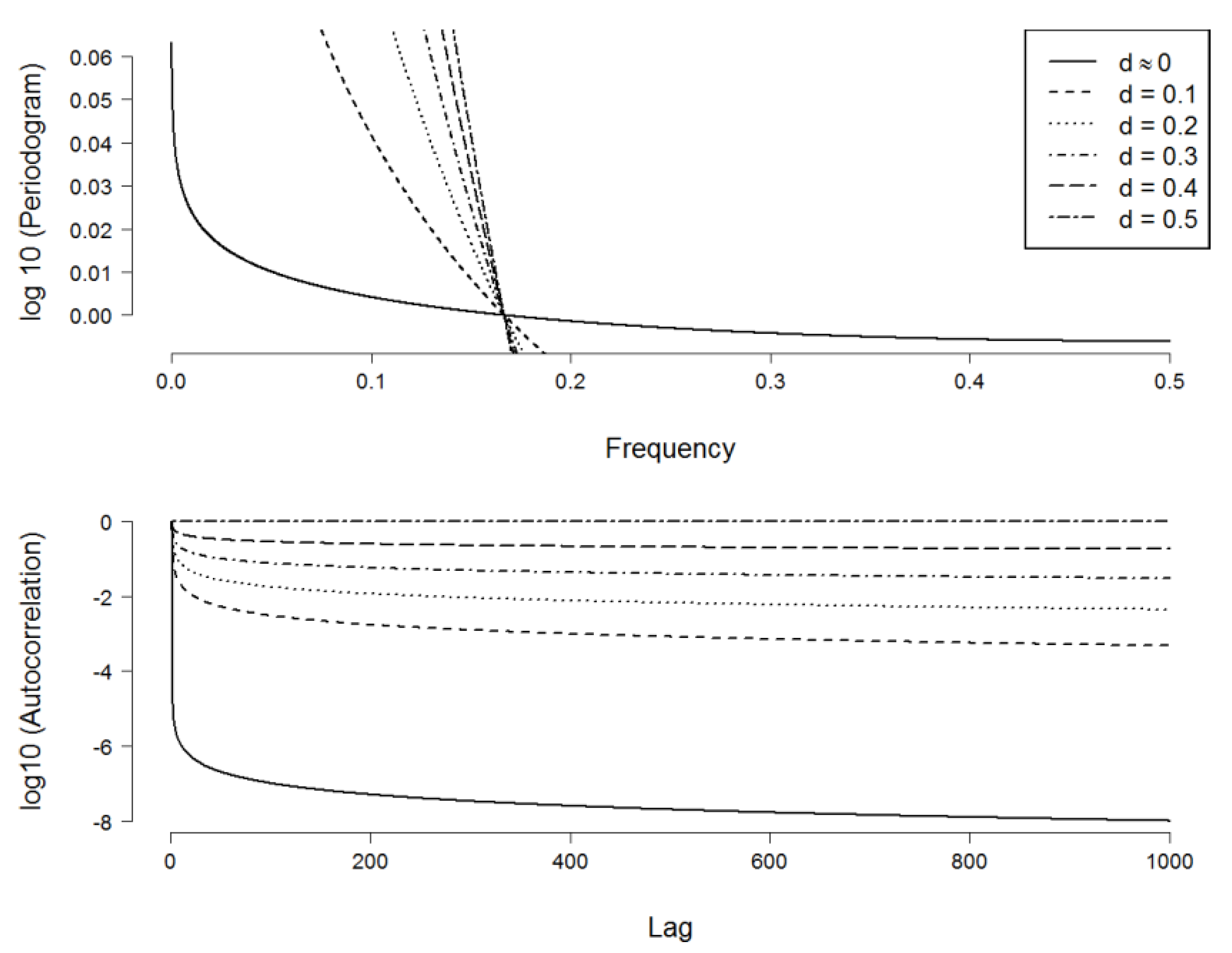
The SDFs of the process with different values of d (and standard normal innovations, i.e., ${\mathsf{\sigma }}^2=1$) are plotted in Figure 1. When $0<d<0.5$ (i.e., long memory exists), the slope of the SDF on a log-log scale increases as d increases. In this case, the SDF has an asymptote at frequency zero, or it is “unbounded at the origin”, in [36]’s terminology. In other words, $S\left(f\right) \to \infty$ when $f \to 0$. Correspondingly, the auto-correlation function (hereafter, ACF) decays more slowly as d increases. While the ACF of a process with $d\approx 0$ quickly dissipates after a small number of lags, the ACF of a process at the ‘high-end’ of the long-memory family, with $d =0.5$, effectively persists at long lags. The former was commonly interpreted as exhibiting “short-memory” behavior.

We can see the relationship between auto-covariance and the spectrum: the ACF decreasing towards very long lags, which correspond to very low frequencies (as the observations are separated by a great time distance, i.e., the wavelength of the periodic signal becomes very high). This reminds us that the spectrum is simply a “representation” of the autocorrelation function in the frequency domain. In addition, Figure 1 shows that the higher the degree of long-memory (the higher the $\mathrm{d}$ parameter), the larger the spectrum will be when $\mathrm{f}\to 0$. It was well-established that both slowly decaying auto-correlation and unbounded spectrum at the origin independently characterize long-memory behavior (see, e.g., [37,38]). In line with these authors, [39] agrees that the pattern of power concentrates at low frequencies and exponentially declines as frequency increases, such as the ones in the top plot of Figure 1, which is the “typical shape” of an economic variable. An important remark that should be made from this observation is that since the periodogram is very high at low frequencies, it is the low frequencies components of a long-memory process that contribute the most to the dynamics of the whole process. For our purposes, we show that to understand the underlying mechanism of risk process, emphasis needs to be placed in the activities of investors with long trading horizons rather than the day-to-day, noisy activities of, for example, market makers.

To avoid the burden of computing the exact likelihood, [2] utilize an approximation to the covariance matrix obtained via the discrete wavelet transformation (hereafter, the DWT): let $\left\{X_t\right\}$ be a fractional difference process with dyadic length $N = 2^j$ and covariance matrix ${\displaystyle \sum }_X$, the likelihood function is defined as:

$$L\left(d, {\sigma }_z^2|X\right)=2{\pi }^{N/2}{\left|{\Sigma }_X\right|}^{-1/2}\exp \left[-\frac{1}{2}{X}^T{\Sigma }_X^{-1}X\right],$$

(5)

where $\left|{\Sigma }_X\right|$ denotes the determinant of ${\Sigma }_X$. Furthermore, we have the approximate covariance matrix given by ${\Sigma }_X\approx {\hat{\Sigma }}_X=W^{\prime }{\Omega }_{N}W$, where $W$ is the orthonormal matrix representing the DWT. ${\Omega }_N$ is a diagonal matrix which contains the variances of DWT coefficients. The approximate likelihood function and its logarithm are:

$$\widehat{L}\left(d, {\sigma }_z^2|X\right)={\left(2\pi \right)}^{-\frac{N}{2}}{\left|\widehat{{\Sigma }_X}\right|}^{-\frac{1}{2}}\exp \left[-\frac{1}{2}{X}^T{\widehat{{\Sigma }_X}}^{-1}X\right]$$

(6)

$$\log \widehat{L}\left(d, {\sigma }_z^2|X\right)=-2 \log \widehat{L}\left(d, {\sigma }_z^2|X\right)-N\log \left(2\pi \right)=\log \left(\left|{\widehat{\Sigma }}_X\right|\right)+X^T{\widehat{{\Sigma }_X}}^{-1}X.$$

(7)

As noted earlier, [1] introduced the wavelet variance $S_j$ for scale ${\lambda }_j$ which satisfies $S_j(d,{\mathsf{\sigma }}_{\mathrm{z}}^2)={\mathsf{\sigma }}_{\mathrm{z}}^2{S}_j^{\prime } \left(d\right)$. The properties of diagonal and orthonormal matrices allow us to rewrite the approximate log-likelihood function in Equation (1) as:

$$\begin{gathered} \widehat{L}\left(d, {\sigma }_z^2|X\right)=N\log \left({\sigma }_z^2\right)+\log \left[S_{J+1}^{\prime }\left(d\right)\right]+{\Sigma }_{j=1}^J{N}_j\log \left[S_j^{\prime }\left(d\right)\right]+\frac{1}{{\sigma }_z^2}\left[\frac{v_J^T{v}_J}{S_{J+1}^{\prime }\left(d\right)}+ \\ {{\displaystyle \sum }}_{j=1}^J\frac{w_j^T{w}_j}{S_j^{\prime }\left(d\right)}\right]. \end{gathered}$$

(8)

The maximum likelihood procedure requires us to find the values of $d$ and ${\sigma }_z^2$ to minimize the log-likelihood function. To do this, we set the differentiated Equation (2) (with respect to ${\sigma }_z^2$) to zero and then find the MLE of ${\sigma }_z^2$:

$${\widehat{\sigma }}_{\mathrm{z}}^2=\frac{1}{\mathrm{N}}\left[\frac{v_J^T{v}_J}{S_{J+1}^{\prime }\left(d\right)}+{{\displaystyle \sum }}_{j=1}^{\mathrm{J}}\frac{w_j^T{w}_j}{S_j^{\prime }\left(d\right)}\right].$$

(9)

Finally, we put this value into Equation (2) to get the reduced log-likelihood, which is a function of the parameter d:

$$\widehat{L}\left(d, {\sigma }_z^2|X\right)=N\log \left({\sigma }_z^2\right)+\log \left[S_{J+1}^{\prime }\left(d\right)\right]+{\Sigma }_{j=1}^J{N}_j\log \left[S_j^{\prime }\left(d\right)\right].$$

(10)

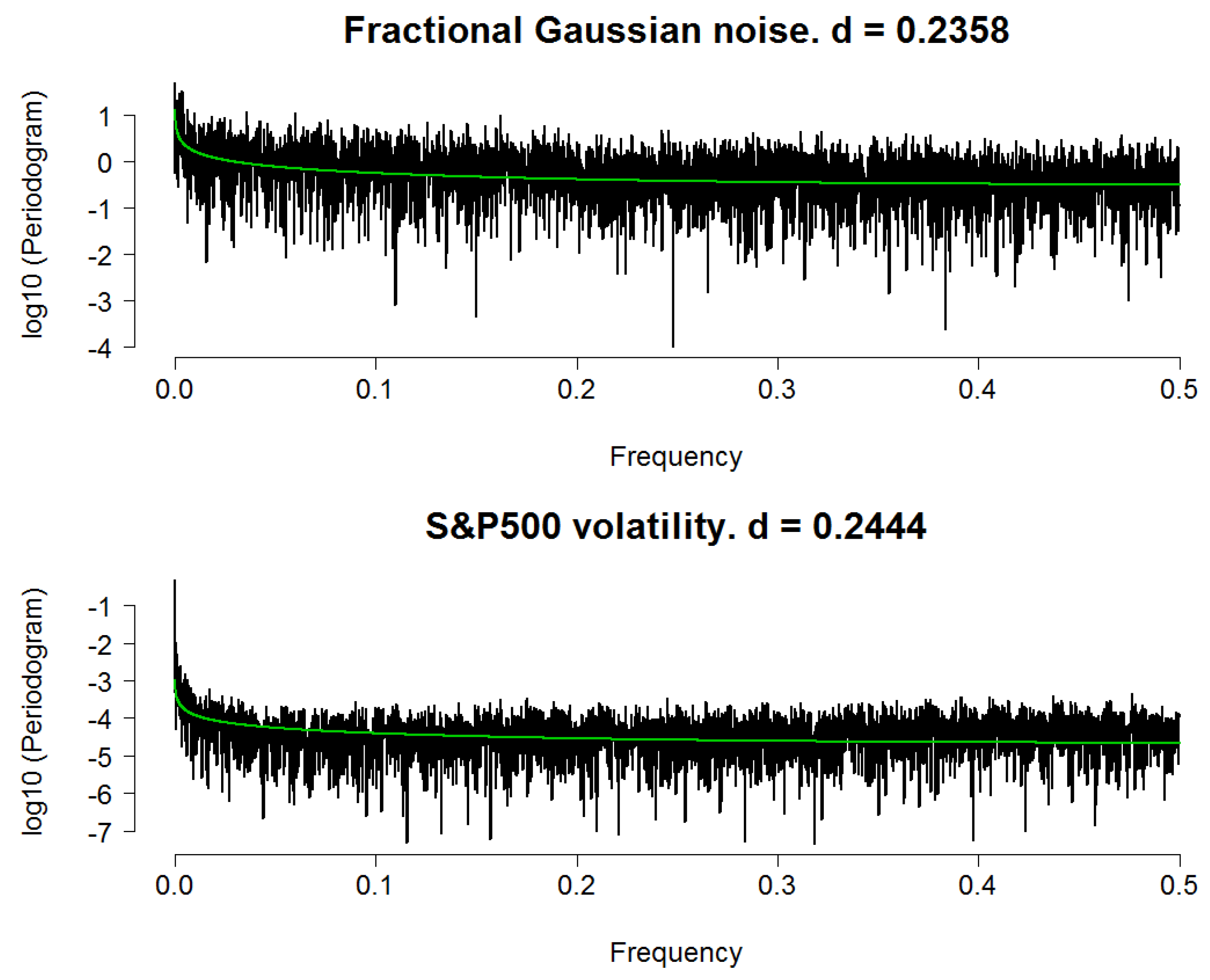
As an illustration, we apply the wavelet MLE to our simulated fGn dataset with H = 0.7 and the volatility series of S&P500 index (proxied by daily absolute returns). Because a dyadic length signal is crucial for this experiment, we obtain daily data ranges from 6 February 1981 to 31 July 2013 (from http://finance.yahoo.com), for a total of 8192 = 213 working days. In addition, we set the number of simulated fGn observations equals to 8192 for comparison. We chose an LA8 wavelet with the decomposition depth set to 13 levels. Figure 2 summarizes our results. Because the actual values of the SDF are very small, we substitute them with their base-10 logarithmic transformation to make the plot visually clear. Estimates of d are 0.2435 and 0.2444 (corresponding to H = 0.7435 and H = 0.7444) for the simulated fGn and S&P500 daily risk processes, respectively. Corresponding values of ${\hat{\mathsf{\sigma }}}^2$ (or the residuals’ variance) are $0.8359$ and $6.2236\times {10}^{-5}$. Subsequently, we have the corresponding time series models:

$${\left(1 - L\right)}^{0.2435}{X}_t = z_t\mathrm{with} z_t \sim i.i.d N\left(0, 0.8359\right)$$

(11)

$${\left(1 - L\right)}^{0.2444}\left|r_t\right|= u_t \mathrm{with} u_t \sim i.i.d N \left(0, 6.2236 \times {10}^{-5}\right).$$

(12)

To further demonstrate the ability of our estimator in capturing long-memory behavior, for each case we plot the theoretical SDF of a fractional difference process with a parameter d set to equal that of the estimated value. Then, we fit this SDF (indicated by a green line) with the corresponding periodogram/spectral density function obtained from the data. In line with [1]’s findings, for both cases the two spectra are in good agreement in terms of overall shape, save for some random variation. However, we obtain a much smaller value of ${\hat{\mathsf{\sigma }}}_{\mathrm{z}}^2$ for the S&P500 series, thus random variation is less severe in its case. In other words, the green line approximates the spectrum of the risk series better than in the case of the fGn. In summary, it can be concluded that this method is effective regarding detecting long-range dependence. The result also indicates that the daily S&P500 volatility series can be reasonably modelled as an fGn process since the two have very similar long-memory parameter.

4. Estimators’ Performance Comparison

In Section 2 and Section 3, we introduced a plethora of estimating methods for long-memory parameter. In this section, we compare their performance, especially against the wavelet-based MLE. We follow [34]’s framework for comparing the performance of described methodologies: first, we simulate N = 500 realizations of the long-memory processes [i.e., fBm, fGn, FARIMA (0, d, 0) and ARFIMA (1, d, 1)], each realization will have a length of 10,000 (which makes it a dyadic length time series) and is generated with the Hurst exponent set to H = 0.7. Then we applied all 9 estimators to each realization, to obtain a sample of 500 estimates of H for each of the methods.

Next, we compute the sample mean, standard deviation and the square root of the mean squared error (MSE) for each sample as follows:

$$\overline{H}=\frac{1}{N}\left({{\displaystyle \sum }}_{n=1}^N{H}_n\right),$$

(13)

$$\widehat{\sigma }=\sqrt{\frac{1}{N-1}\left[{{\displaystyle \sum }}_{n=1}^N{H}_n^2-\frac{1}{N}{\left({{\displaystyle \sum }}_{n=1}^N{H}_n\right)}^2\right]},$$

(14)

$$\sqrt{MSE}=\sqrt{\frac{1}{N}{{\displaystyle \sum }}_{n=1}^N{\left(H_n-H\right)}^2},$$

(15)

where $H_n$ is the estimate of Hurst index obtained from the n-th (simulated) realization of each process in each sample. Similar to conventional estimating techniques, here the standard error indicates the significance of the estimator while the mean squared error measures its performance by comparing it with the nominal value. We repeat this procedure with $H = 0.5$ and $H = 0.9$ (approximately representing the lower and upper bounds of the Hurst exponent for the stationary long-memory class). For comparative purpose, we also estimate H for a sample of 50 realizations ($N = 50$) as done by [34]. We noted that the MSE incorporate an indicator of bias within our simulated samples that can be expressed as: $MSE=Sample variance+Bia{s}^2={\sigma }^2+{\left(\overline{H}-H\right)}^2$ so that the estimator yielding the smallest value of $\sqrt{MSE}$ is considered to have the best performance.

The results for the simulation experiment with the fGn and FARIMA (0, d, 0) (for which $\widehat{H}=\widehat{d}+0.5$) are reported in

Table 2. Performance comparison for different long-memory estimators.

		Fractional Gaussian Noise						FARIMA (0, d, 0)
		H = 0.5		H = 0.7		H = 0.9		H = 0.5		H = 0.7		H = 0.9
Method	Measurement	N = 50	N = 500	N = 50	N = 500	N = 50	N = 500	N = 50	N = 500	N = 50	N = 500	N = 50	N = 500
R/S	$\overline{H}$	0.564	0.563	0.717	0.713	0.823	0.830	0.560	0.571	0.682	0.703	0.846	0.828
	$\widehat{\sigma }$	0.068	0.084	0.094	0.088	0.089	0.094	0.083	0.085	0.079	0.089	0.110	0.090
	$\sqrt{MSE}$	0.093	0.105	0.095	0.089	0.117	0.117	0.101	0.111	0.081	0.089	0.121	0.115
aggVar	$\overline{H}$	0.493	0.498	0.685	0.684	0.847	0.843	0.495	0.496	0.690	0.686	0.844	0.843
	$\widehat{\sigma }$	0.025	0.027	0.030	0.029	0.034	0.030	0.030	0.028	0.028	0.030	0.032	0.029
	$\sqrt{MSE}$	0.025	0.027	0.033	0.033	0.063	0.064	0.031	0.028	0.030	0.033	0.064	0.063
diffaggVar	$\overline{H}$	0.508	0.518	0.715	0.710	0.899	0.902	0.515	0.511	0.719	0.706	0.901	0.900
	$\widehat{\sigma }$	0.064	0.061	0.054	0.055	0.059	0.057	0.050	0.055	0.057	0.055	0.059	0.056
	$\sqrt{MSE}$	0.064	0.064	0.056	0.056	0.058	0.057	0.052	0.056	0.060	0.055	0.059	0.056
AbaggVar	$\overline{H}$	0.498	0.502	0.691	0.690	0.853	0.849	0.497	0.501	0.695	0.692	0.850	0.849
	$\widehat{\sigma }$	0.026	0.028	0.030	0.031	0.034	0.032	0.031	0.029	0.031	0.031	0.033	0.032
	$\sqrt{MSE}$	0.026	0.028	0.031	0.032	0.057	0.060	0.031	0.029	0.031	0.032	0.060	0.060
Per	$\overline{H}$	0.497	0.501	0.705	0.706	0.912	0.912	0.498	0.499	0.705	0.704	0.908	0.909
	$\widehat{\sigma }$	0.019	0.022	0.020	0.020	0.021	0.021	0.019	0.022	0.019	0.022	0.021	0.021
	$\sqrt{MSE}$	0.019	0.022	0.020	0.021	0.024	0.024	0.019	0.022	0.020	0.022	0.023	0.023
modPer	$\overline{H}$	0.451	0.456	0.662	0.664	0.869	0.870	0.452	0.454	0.660	0.658	0.863	0.860
	$\widehat{\sigma }$	0.023	0.022	0.024	0.022	0.024	0.022	0.020	0.023	0.023	0.022	0.023	0.022
	$\sqrt{MSE}$	0.054	0.049	0.045	0.042	0.039	0.037	0.052	0.052	0.046	0.047	0.044	0.045
Peng	$\overline{H}$	0.489	0.491	0.688	0.688	0.886	0.885	0.487	0.489	0.676	0.677	0.873	0.874
	$\widehat{\sigma }$	0.015	0.012	0.015	0.015	0.018	0.016	0.013	0.012	0.015	0.016	0.017	0.017
	$\sqrt{MSE}$	0.018	0.015	0.019	0.019	0.022	0.022	0.019	0.016	0.028	0.028	0.032	0.031
Higuchi	$\overline{H}$	0.474	0.478	0.670	0.670	0.860	0.857	0.473	0.476	0.675	0.670	0.865	0.859
	$\widehat{\sigma }$	0.017	0.019	0.025	0.025	0.036	0.042	0.023	0.020	0.029	0.026	0.044	0.041
	$\sqrt{MSE}$	0.031	0.029	0.039	0.039	0.053	0.060	0.035	0.031	0.039	0.040	0.056	0.058
waveMLE	$\overline{H}$	0.497	0.501	0.725	0.726	0.915	0.915	0.500	0.500	0.694	0.694	0.895	0.891
	$\widehat{\sigma }$	0.008	0.008	0.008	0.008	0.017	0.017	0.009	0.008	0.009	0.008	0.024	0.021
	$\sqrt{MSE}$	0.008	0.008	0.027	0.027	0.023	0.022	0.009	0.008	0.011	0.010	0.024	0.023

Notes: Nomenclatures of the methods are as follows: (1) R/S: rescaled range [10]; (2) aggVar: aggregated variance [24]; (3) diffaggVar: differenced variance [31]; (4) AbaggVar: absolute moments [31]; (5) Per: periodogram [34]; (6) modPer: modified periodogram [34]; (7) Peng: regression of residuals [33]; (8) Higuchi: Higuchi’s method [32]; (9) waveMLE: wavelet-based maximum likelihood [2]. To preserve space, we do not present the results for fBm and ARFIMA (p, d, q), which are qualitatively similar to those reported and are available upon request.

. There are several observations that can be made from this table:

• All of the proposed methods seem to estimate parameter H effectively, in that they can detect the dependence structure of the simulated time series, with relatively small standard errors.
• The values of $\overline{H}$, $\widehat{\sigma }$ and $\sqrt{MSE}$ do not differ significantly between the cases of N = 50 and N = 500.
• The rescaled range method yields the least desirable performance in all simulated experiments. This is in contrast to many previous studies supporting the use of this method, yet it is in line with skeptics such as [34].

When examining Table 2, we can see that the wavelet-based MLE performs relatively robustly compared to several other methods. In particular, in the case of the simulated fGn, when $H = 0.5$ (i.e., when the process becomes a Brownian motion) waveMLE is superior. For a “typical” long-memory process ($H = 0.7$) waveMLE ranks third, and for process exhibiting extreme long-range dependence behaviour ($\mathrm{H}=0.9$) this estimator ranks second. When it comes to the FARIMA (0, d, 0) process, waveMLE performs best in all cases. We illustrate these arguments by presenting the rankings based on the MSE (with $N = 500$) in

Table 3. Performance of long-memory estimators.

Fractional Gaussian Noise
Method	H = 0.5	Method	H = 0.7	Method	H = 0.9
waveMLE	0.00809	Peng	0.01948	Peng	0.0217846
Peng	0.015141	Per	0.021326	waveMLE	0.0223977
Per	0.021721	waveMLE	0.027468	Per	0.0237573
aggVar	0.0267	AbaggVar	0.032387	modPer	0.0372976
AbaggVar	0.027645	aggVar	0.033436	diffaggVar	0.0567174
Higuchi	0.029087	Higuchi	0.039072	Higuchi	0.0598122
modPer	0.049141	modPer	0.042152	AbaggVar	0.0602138
diffaggVar	0.063601	diffaggVar	0.055628	aggVar	0.0641194
R/S	0.105121	R/S	0.089366	R/S	0.1170989
FARIMA (0, d, 0)
Method	H = 0.5	Method	H = 0.7	Method	H = 0.9
waveMLE	0.008196	waveMLE	0.010249	waveMLE	0.0227378
Peng	0.016386	Per	0.021878	Per	0.0228976
Per	0.021512	Peng	0.028202	Peng	0.0314989
aggVar	0.028119	AbaggVar	0.032151	modPer	0.0452348
AbaggVar	0.029126	aggVar	0.033022	diffaggVar	0.0557743
Higuchi	0.031394	Higuchi	0.039716	Higuchi	0.0581878
modPer	0.051638	modPer	0.047401	AbaggVar	0.0602195
diffaggVar	0.055694	diffaggVar	0.055482	aggVar	0.0634601
R/S	0.110746	R/S	0.08907	R/S	0.1150482

Notes: The methods are ordered based on increasing MSE. The statistic is calculated from a sample of 500 estimates for each method. Nomenclatures are similar to those specified in Table 2.

.

Additionally, when $H = 0.5$ and $H = 0.7$ (corresponding to the value generally expected to be observed in financial returns and financial risk time series, respectively) wave MLE provides the smallest value of MSE on average, which is also smaller than those obtained when estimating $H = 0.9$ (which is unlikely to be observed). Furthermore, in cases where waveMLE is not the best estimator, the difference between its performance and that of the best estimator is not significant. For example, in the case of fGn with $H = 0.7$ and $H = 0.9$ this difference is only measured by units of 0.1%. To see how important this is, consider the performance of the Peng method (which outperforms waveMLE in these cases): when the Peng method is not the best, the difference between its performance and the best estimator (waveMLE) is in units of 1%.

It can be concluded that waveMLE is rarely seen being beaten by another estimator, and when it is, it does not get beaten by a large margin. Nevertheless, with all evidence in clear favor of waveMLE, in practice we still need to take into account the main limitation of this seemingly superior estimator, that is, it can only be applied on a dyadic length time series.

5. Application to Fossil Fuel Prices

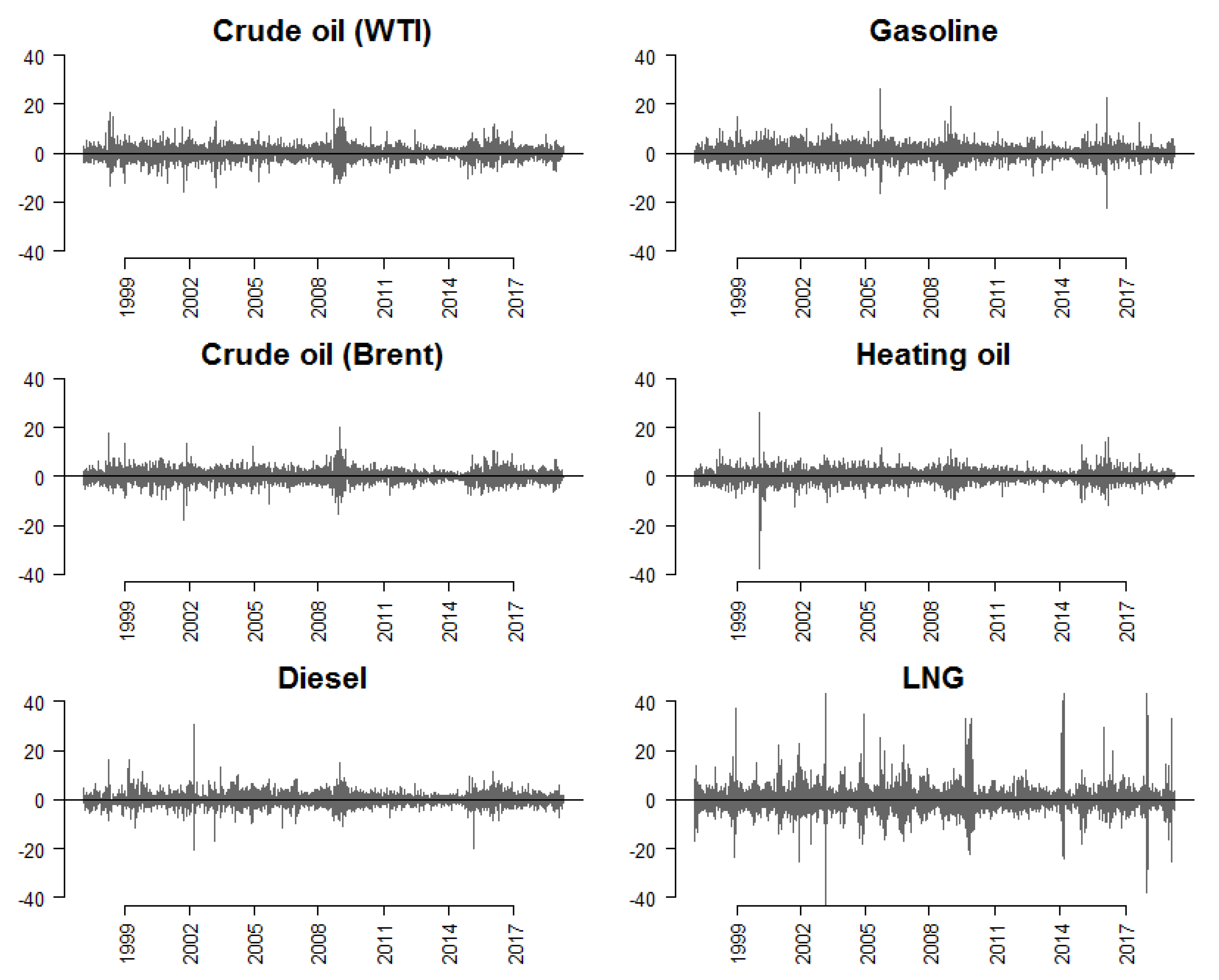
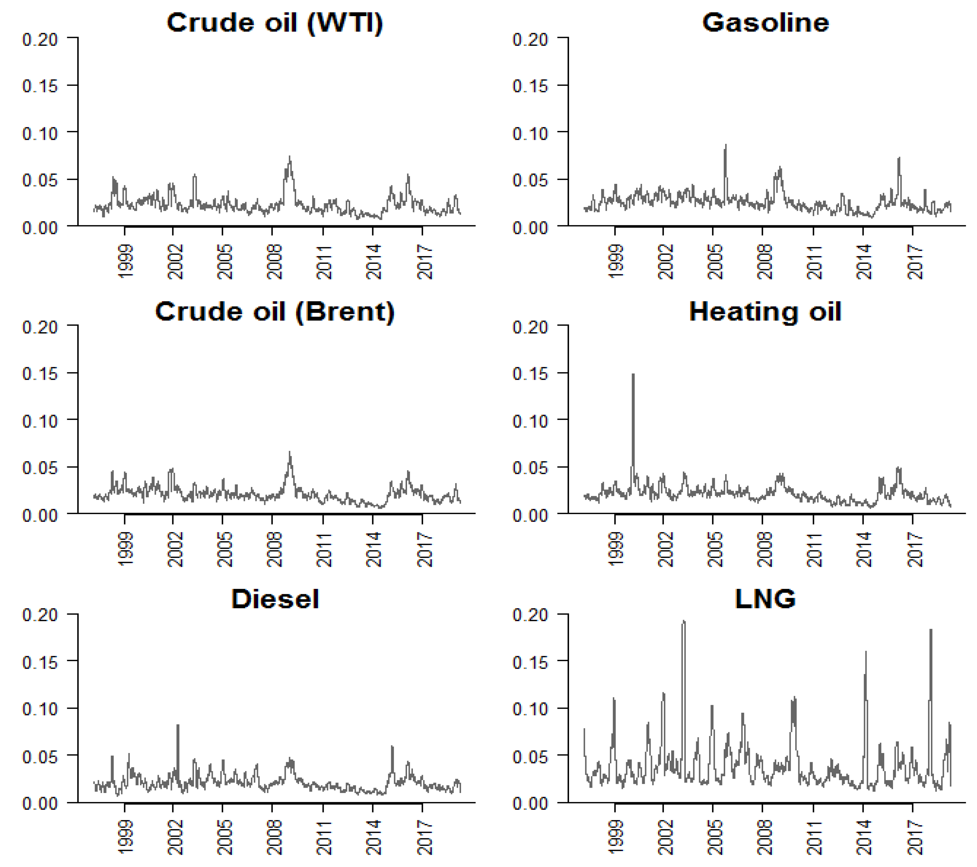
In this section, we apply the methodology discussed in Section 3 to examine the characteristics of fuel price time series. Our data are the spot prices of six commodities: crude oil [West Texas Intermediate (WTI)], crude oil (Brent – Europe), diesel fuel (Los Angeles Ultra-Low-Sulfur No. 2), gasoline (New York Harbor conventional), heating oil (New York Harbor No. 2), and liquid natural gas (LNG) (Henry Hub). The data are provided by [40] and range from 9 January 1997 to 22 April 2019. We compute daily spot returns as $r_{it}=\log p_{it}-\log p_{i,t-1} \left(t=1,\dots ,T\right)$, where $p_{it}$ denotes the spot price of commodity i and $T=5535$ denotes the number of observations. The corresponding volatility series are computed as 30-day rolling standard deviations of returns, i.e., ${\sigma }_{it}=\sqrt{\left(1/30\right){{\displaystyle \sum }}_{j=2}^{31}{\left[\left(\log p_{i,t+j}-\log p_{i,t+j-1}\right)-{\overline{r}}_{it}\right]}^2}$ where ${\overline{r}}_{it}=\left(1/30\right){{\displaystyle \sum }}_{j=2}^{31}\left(\log p_{i,t+j}-\log p_{i,t+j-1}\right)$ is the rolling average return. As can be seen in Figure 3, of the six commodity returns examined, natural gas seems to yield the most volatile returns, at times exceeding 40%. This is also shown in the corresponding volatility plot presented in the bottom-right panel of Figure 4. Visual inspection of Figure 3 reveals that returns time series exhibit characteristics of white-noise processes.

The summary statistics for return and volatility time series are reported in

Table 4. Summary statistics of returns and volatilities.

	Crude Oil (WTI)	Crude Oil (Brent)	Diesel	Gasoline	Heating Oil	LNG
A. Returns
Mean	0.00	0.00	0.00	0.00	0.00	0.00
Median	0.00	0.00	0.00	0.00	0.00	0.00
Variance	0.00	0.00	0.00	0.00	0.00	0.00
Skewness	−0.11	−0.07	0.09	−0.02	−1.30	0.53
Kurtosis	4.48	4.85	10.96	5.75	36.58	23.36
JB	4,636.39	5,425.09	27,726.50	7,626.17	31,0451.74	12,6236.23
	(0.00)	(0.00)	(0.00)	(0.00)	(0.00)	(0.00)
LB(21)	49.22	52.96	58.48	59.98	63.28	269.94
	(0.00)	(0.00)	(0.00)	(0.00)	(0.00)	(0.00)
B. Volatilities
Mean	0.02	0.02	0.02	0.03	0.02	0.04
Median	0.02	0.02	0.02	0.02	0.02	0.03
Variance	0.00	0.00	0.00	0.00	0.00	0.00
Skewness	1.78	1.43	2.21	2.02	5.69	2.94
Kurtosis	4.35	3.59	8.77	7.93	52.33	11.73
JB	7,253.17	4,820.13	22,147.27	18,174.67	65,8570.09	39,502.69
	(0.00)	(0.00)	(0.00)	(0.00)	(0.00)	(0.00)
LB(21)	87,932.64	87,228.02	75,212.60	77,604.79	76,836.39	72,836.22
	(0.00)	(0.00)	(0.00)	(0.00)	(0.00)	(0.00)

Notes: Returns of commodity i are computed as the log-change of the corresponding daily spot price: $r_{it}=\log p_{it}-\log p_{i,t-1} \left(t=1,\dots ,T\right)$, where $p_{it}$ denotes the spot price of commodity i. $T$ denotes the number of observations (5535 trading days, from 9 January 1997, to 22 April 2019 ). Volatilities are defined as the 30-day rolling standard deviation of the log-change in prices, i.e., ${\sigma }_{it}=\sqrt{\left(1/30\right){{\displaystyle \sum }}_{j=2}^{31}{\left[\left(\log p_{i,t+j}-\log p_{i,t+j-1}\right)-{\overline{r}}_{it}\right]}^2}$, where ${\overline{r}}_{it}=\left(1/30\right){{\displaystyle \sum }}_{j=2}^{31}\left(\log p_{i,t+j}-\log p_{i,t+j-1}\right)$ is the rolling average return. JB and LB (21) denote the Jarque-Bera (which tests the null of normal distribution) and the Ljung-Box statistics (which tests for the null of no serial autocorrelation up to lag 21), respectively. p-values of these tests are in parentheses.

. We can see that all returns series have a zero mean and a symmetric, leptokurtic distribution (as the Jarque-Bera statistics indicate that the null of normal distribution are strongly rejected). Volatilities have non-zero mean and yield even stronger evidence of serial correlations. Additionally, they also exhibit serial correlation, as the null of independent observations is also strongly rejected as shown by the portmanteau Ljung-Box statistics. These dependence patterns over time imply that the energy spot markets may not be efficient.

In

Table 5. Stationarity tests for returns and volatilities.

	Crude Oil (WTI)	Crude Oil (Brent)	Diesel	Gasoline	Heating Oil	LNG
	A. Returns
ADF	−16.90	−16.88	−17.43	−16.28	−18.76	−19.78
	(0.01)	(0.01)	(0.01)	(0.01)	(0.01)	(0.01)
PP	−5402.46	−5459.67	−6006.09	−5192.76	−5566.76	−4420.88
	(0.01)	(0.01)	(0.01)	(0.01)	(0.01)	(0.01)
KPSS	0.08	0.08	0.05	0.05	0.07	0.03
	(0.10)	(0.10)	(0.10)	(0.10)	(0.10)	(0.10)
	B. Volatilities
ADF	−6.32	−6.59	−8.29	−8.89	−9.36	−10.14
	(0.01)	(0.01)	(0.01)	(0.01)	(0.01)	(0.01)
PP	−60.94	−65.79	−99.93	−97.12	−94.14	−101.89
	(0.01)	(0.01)	(0.01)	(0.01)	(0.01)	(0.01)
KPSS	1.90	3.44	1.94	4.04	2.95	0.39
	(0.01)	(0.01)	(0.01)	(0.01)	(0.01)	(0.08)

Notes: See notes to Table 4. ADF, PP, and KPSS refer to the augmented Dickey-Fuller [41] and Phillips-Perron [42] tests for the null of unit root, and the Kwiatkowski et al. [43] test for the null of stationarity, respectively. p-values of these tests are in parentheses.

, we provide the results of the test for stationarity of returns and volatilities. As can be seen from panel A, all returns series exhibit stationarity, since the null of unit root can be rejected strongly at the 1% significance level (using the Augmented Dickey-Fuller (ADF) [41] and Phillips-Perron (PP) [42] tests) while the null of stationary cannot be rejected at conventional significance levels (using the Kwiatkowski et al. (KPSS) [43] test). Results for volatilities, on the other hand, are mixed: while the ADF and PP tests rule out the existence of unit roots, the KPSS test show evidence of non-stationarity. A possible explanation for the contrasting results is that long-memory of volatilities lower the power of these tests. For example, time series with long-range dependence, as opposed to infinite dependence and following the random walk, may still be stationary.

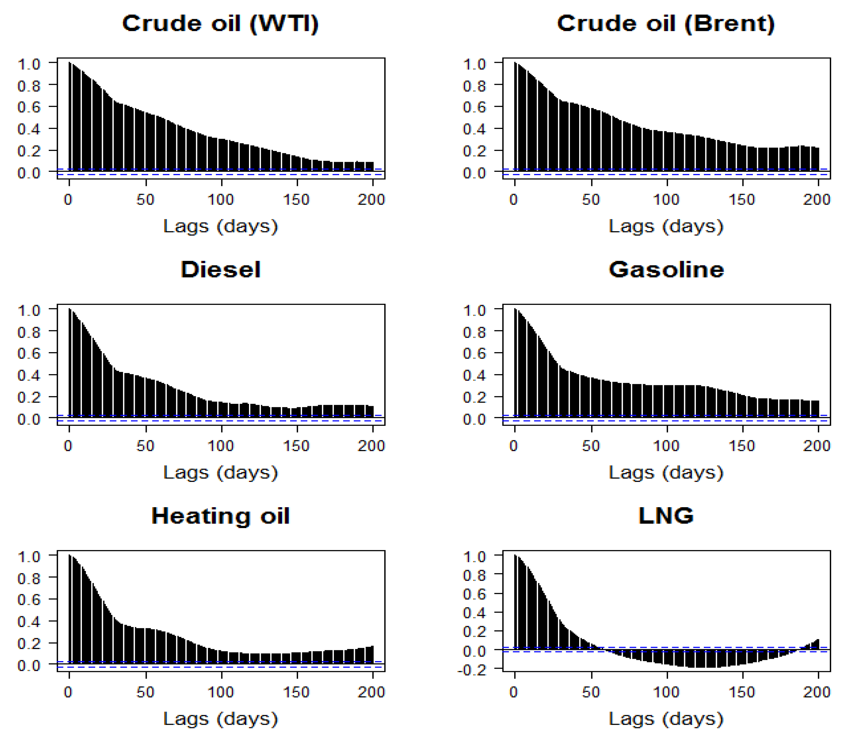
Figure 5 sheds light on this issue by presenting the auto-correlation functions (ACF) of the volatility series. The auto-correlation coefficients are all highly significant even at the 200-day lag (i.e., close to a full trading year). Based on these observations, in

Table 6. Estimates of Hurst exponents with waveMLE.

	Crude Oil (WTI)	Crude Oil (Brent)	Diesel	Gasoline	Heating Oil	LNG
Returns	0.5	0.48	0.51	0.54	0.52	0.38
Volatilities	0.79	0.8	0.77	0.79	0.79	0.78

we present the estimated Hurst exponents for the 6 returns and volatilities series. All returns yield values are in the proximity of 0.4–0.5, while volatilities’ values are in the range of 0.7–0.8. According to the implications of Hurst index on the statistical property of time series (see Table 1), these results support our observation that energy price returns exhibit behavior of white-noise processes while volatilities show evidence of long-memory, which is in agreement with observations previously made in the literature (see, e.g., [18,23]).

6. Conclusions, Implications and Qualifications

Burning fossil fuels, the main source of man-made carbon dioxide, is the most important cause of climate change. Contributing to this issue is the recently lower energy prices and quickly rising share of middle-class population in developing economies, which significantly lifts the global energy consumption rate via the use of personal transportation vehicles [44,45]. Given the importance of prices in determining the supply and demand of energy commodities, it is crucial to develop tools to measure the risk associated with markets for these commodities, to better understand what ultimately affects progress on reducing the adverse effects of climate fluctuations.

This paper contributes to the existing literature by examining various estimation methods for long-memory in price returns and volatilities to assess energy market efficiency. We first investigate the performance of the various conventional methods reviewed by [34] and the wavelet-based maximum likelihood estimator (waveMLE) proposed by [2]. Our simulations indicate that waveMLE is superior to the majority of other methods. Applications of waveMLE support white-noise behavior for returns and long-range dependence for volatility. Our findings offer market participants an interesting opportunity to exploit potential inefficiency in the energy markets. For example, policy makers can prepare to provide stricter price regulation when there are volatility spikes that tend to be prolonged, while traders can design optimal hedging strategies based on forecasts of future volatilities that incorporate long-memory.

Our findings are subject to two qualifications. First, potential structural breaks in fossil fuel prices are not covered in our analyses. However, given the robust evidence of long-memory detected for volatilities in previous studies even in the presence of such breaks (see, e.g., [16,17,18]), we conjecture that these breaks are not a major source of bias for our primary findings. Second, we have not investigated the forecasting value of our estimators, which could potentially offer further important implications for the understanding of energy market dynamics. This will be an interesting future research direction.

References

- Hurst, H. Long term storage capacity of reservoirs. Trans. Am. Soc. Civ. Eng. 1951, 116, 770–799. [Google Scholar]
- Gencay, R.; Selcuk, F.; Whitcher, B. An Introduction to Wavelets and Other Filtering Methods in Finance and Economics; Academic Press: San Diego, CA, USA, 2002. [Google Scholar]
- Samuelson, P.A. Proof that Properly Anticipated Prices Fluctuate Randomly. Ind. Manag. Rev. 1965, 6, 41–49. [Google Scholar]
- Fama, E.F. The Behavior of stock market prices. J. Bus. 1965, 38, 34–105. [Google Scholar] [CrossRef]
- Lo, A.W. Long-term memory in stock market prices. Econometrica 1991, 59, 1279–1313. [Google Scholar] [CrossRef]
- Jennergren, L.P.; Korsvold, P.E. Price formation in the Norwegian and Swedish stock markets: Some random walk tests. Swedish J. Econ. 1974, 76, 171–185. [Google Scholar] [CrossRef]
- Cootner, P.H. Common Elements in Futures Markets for Commodities and Bonds. Am. Econ. Rev. 1961, 51, 173–183. [Google Scholar]
- Fama, E.F.; French, K.R. Permanent and temporary components of stock prices. J. Polit. Econ. 1988, 96, 246–273. [Google Scholar] [CrossRef]
- Ding, Z.; Granger, C.W.J.; Engle, R.F. A long memory property of stock market returns and a new model. J. Empir. Finance 1993, 1, 83–106. [Google Scholar] [CrossRef]
- Andersen, T.G.; Bollerslev, T. Heterogeneous information arrivals and return volatility dynamics: Uncovering the long run in high frequency returns. J. Finance 1997, 52, 975–1005. [Google Scholar] [CrossRef]
- Mandelbrot, B.; Wallis, J.R. Noah, Joseph, and operational hydrology. Water Resources Res. 1968, 4, 909–918. [Google Scholar] [CrossRef]
- Peters, E. Chaos and Order in the Capital Markets: A New View of Cycles, Prices, and Market Volatility; John Wiley & Sons: New York, NY, USA, 1996. [Google Scholar]
- Lo, A.W.; MacKinlay, C.A. A Non-Random Walk Down Wall Street; Princeton University Press: Princeton, NJ, USA, 1999. [Google Scholar]
- Hull, M.; McGroarty, F. Do emerging markets become more efficient as they develop? Long memory persistence in equity indices. Emerging Markets Rev. 2013, 18, 45–61. [Google Scholar] [CrossRef]
- Grossman, S.J.; Stiglitz, J.E. On the impossibility of informationally efficient markets. Am. Econ. Rev. 1980, 70, 393–408. [Google Scholar]
- Lo, A.W. The adaptive markets hypothesis: Market efficiency from an evolutionary perspective. J. Portfolio Manag. 2004, 30, 15–29. [Google Scholar] [CrossRef]
- Choi, K.; Hammoudeh, S. Long memory in oil and refined products markets. Energy J. 2009, 30, 97–116. [Google Scholar] [CrossRef]
- Baillie, R.; Han, Y.-W.; Myers, R.; Song, J. Long memory models for daily and high frequency commodity futures returns. J. Futures Markets 2007, 27, 643–668. [Google Scholar] [CrossRef]
- Arouri, M.E.H.; Lahiani, A.; Lévy, A.; Nguyen, D.K. Forecasting the conditional volatility of oil spot and futures prices with structural breaks and long memory models. Energy Econ. 2012, 34, 283–293. [Google Scholar] [CrossRef]
- Charfeddine, L. True or spurious long memory in volatility: Further evidence on the energy futures markets. Energy Policy 2014, 71, 76–93. [Google Scholar] [CrossRef]
- Wang, Y.; Wu, C. Long memory in energy futures markets: Further evidence. Resources Policy 2012, 37, 261–272. [Google Scholar] [CrossRef]
- Di Sanzo, S. A Markov switching long memory model of crude oil price return volatility. Energy Econ. 2018, 74, 351–359. [Google Scholar] [CrossRef]
- Nademi, A.; Nademi, Y. Forecasting crude oil prices by a semiparametric Markov switching model: OPEC, WTI, and Brent cases. Energy Econ. 2018, 74, 757–766. [Google Scholar] [CrossRef]
- Dieker, A.B.; Mandjes, M. On spectral simulation of fractional Brownian motion. Probab. Eng. Informat. Sci. 2003, 17, 417–434. [Google Scholar] [CrossRef]
- Cox, D.R. Long-range Dependence: A Review. In Statistics: An Appraisal, Proceedings of a Conference Marking the 50th Anniversary of the Statistical Laboratory, Iowa State University, Ames, Iowa, 13–15 June 1983; David, H.A., David, H.T., Eds.; Iowa State University Press: Ames, IA, USA, 1984; pp. 55–74. [Google Scholar]
- Beran, J. Statistics for Long-Memory Processes; Chapman and Hall: New York, NY, USA, 1994. [Google Scholar]
- Mandelbrot, B.; Van Ness, J.W. Fractional Brownian motions, fractional noises and applications. SIAM Rev. 1968, 10, 422–437. [Google Scholar] [CrossRef]
- Mitra, S.K. Is Hurst exponent value useful in forecasting financial time series? Asian Soc. Sci. 2012, 8, 111–120. [Google Scholar] [CrossRef]
- Mandelbrot, B. Statistical methodology for nonperiodic cycles: From the covariance to R/S analysis. In Proceedings of the Annals of Economic and Social Measurement; National 579 Bureau of Economic Research: Stanford, CA, USA, 1972; Volume 1, pp. 259–290. [Google Scholar]
- Willinger, W.; Taqqu, M.S.; Teverovsky, V. Stock market prices and long-range dependence. Finance Stochastics 1999, 3, 1–13. [Google Scholar] [CrossRef]
- Teverovsky, V.; Taqqu, M. Testing for long-range dependence in the presence of shifting means or a slowly declining trend, using a variance-type estimator. J. Time Ser. Anal. 1997, 18, 279–304. [Google Scholar] [CrossRef]
- Higuchi, T. Approach to an irregular time series on the basis of the fractal theory. Phys. D Nonlinear Phenomena 1981, 31, 277–283. [Google Scholar] [CrossRef]
- Peng, C.K.; Buldyrev, S.V.; Havlin, S.; Simons, M.; Stanley, H.E.; Goldberger, A.L. Mosaic organization of DNA nucleotides. Phys. Rev. E 1994, 49, 1685–1689. [Google Scholar] [CrossRef]
- Taqqu, M.T.V.; Willinger, W. Estimators for long-range dependence: An empirical study. Fractals 1995, 3, 785–798. [Google Scholar] [CrossRef]
- In, F.; Kim, S. An Introduction to Wavelet Theory in Finance: A Wavelet Multiscale Approach; World Scientific: Singapore, 2013. [Google Scholar]
- Jensen, M.J. An alternative maximum likelihood estimator of long-memory processes using compactly supported wavelets. J. Econ. Dyn. Control 2000, 24, 361–387. [Google Scholar] [CrossRef]
- McLeod, B.; Hipel, K. Preservation of the rescaled adjusted range. Water Resources Res. 1978, 14, 491–518. [Google Scholar] [CrossRef]
- Resnick, S. Extreme Values, Regular Variation, and Point Processes; Springer: New York, NY, USA, 2007. [Google Scholar]
- Granger, C.W.J. The typical spectral shape of an economic variable. Econometrica 1966, 34, 150–161. [Google Scholar] [CrossRef]
- United States Energy Information Administration. Petroleum and other liquids. Available online: https://www.eia.gov/petroleum/data.php (accessed on 18 May 2019).
- Dickey, D.A.; Fuller, W.A. Distributions of the estimators for autoregressive time series with a unit root. J. Am. Stat. Assoc. 1979, 74, 427–431. [Google Scholar]
- Phillips, P.C.B.; Perron, P. Testing for a unit root in time series regression. Biometrika 1988, 75, 335–346. [Google Scholar] [CrossRef]
- Kwiatkowski, D.; Phillips, P.C.B.; Schmidt, P.; Shin, Y. Testing the null hypothesis of stationarity against the alternative of a unit root. J. Econometr. 1992, 54, 159–178. [Google Scholar] [CrossRef]
- Montgomery, S.L. Cheap oil is blocking progress on climate change. The Conversation [online] 2018, 12. Available online: https://theconversation.com/cheap-oil-is-blocking-progress-on-climate-change-108450 (accessed on 28 April 2019).
- Office of Energy Efficiency and Renewable Energy. About Two-Thirds of Transportation Energy Use is Gasoline for Light Vehicles; Office of Energy Efficiency and Renewable Energy: Washington, DC, USA, 2013.
Figure 1.
Spectral density function and ACF of a fractional difference process with various values of . Notes: The higher the fractional difference parameter, the stronger the long-run dependence and the higher the slope of the spectrum. The rate of decay of the corresponding ACF decreases as increases: from very quickly (when , i.e., “short-memory”) to effectively infinite persistence (when ). Note how the asymptote at very low frequencies (in the SDF plot) is associated to the persistence at very big lags (in the ACF plot). Because of scaling factor, the plot of the SDFs seemingly indicates that the SDFs with ‘cut’ the x-axis, although in fact this is not the case. All SDFs exhibit an exponential decaying pattern when plotted on separate scale. The higher the value of , the higher the asymptote near frequency zero and the faster the SDF decays.
Figure 2.
Spectral density functions (on a log 10 scale) of a fractional Gaussian noise process and the daily volatility process of S&P500. Notes: Highest frequency being 0.5 corresponds to the Nyquist frequency. In both plots the green line indicates theoretical spectrum of long-memory process with values of d estimated using the waveMLE method.
Figure 3.
Daily returns of energy commodities, 1997–2019. Notes: Returns of commodity i are computed as the percentage change of the corresponding daily spot price: , where denotes the spot price of commodity i. To facilitate visualization, the vertical range is concatenated at [−40, 40] (%).
Figure 4.
Volatilities of energy commodities, 1997–2019. Notes: Volatilities are defined as the 30-day rolling standard deviation of the log-change in prices, i.e., , where is the rolling average return. denotes the spot price of commodity i.
Figure 5.
Auto-correlograms of volatility of energy commodities, 1997–2019. Notes: Returns of commodity i are computed as the log-change of the corresponding daily spot price: . Volatility is computed as 30-day rolling standard deviations of .