Sustainable Urban Liveability: A Practical Proposal Based on a Composite Indicator


1
Department of Applied Economics, Faculty of Economics and Business Administration, University of Santiago de Compostela, Av. Burgo das Nacións s/n, 15782 Santiago de Compostela, Spain
2
Department of Economics, Business and Economy School, University of A Coruña, Elviña Campus, A Coruña 15071, Spain
*
Author to whom correspondence should be addressed.
Sustainability 2019, 11(1), 86; https://doi.org/10.3390/su11010086
Submission received: 15 November 2018
/
Revised: 17 December 2018
/
Accepted: 19 December 2018
/
Published: 24 December 2018
Abstract
:This article presents a proposal for a composite index to assess the degree of sustainable urban liveability. It makes two key contributions to this field of study. The first is a proposal for the concept of sustainable urban liveability that includes the need to meet a minimum number of environmental conditions in terms of resource consumption and the deterioration of the environment. The second contribution is the use of a non-compensatory aggregation technique in order to construct the composite index. This kind of aggregation technique does not allow trade-offs between partial indicators. In the particular context of sustainable urban liveability, it prevents poor performance by the natural environment indicators from being compensated by positive results in the remaining indicators. The proposed composite index for sustainable urban liveability is applied to the case of 58 Spanish cities. The results reveal significant differences in the degree of sustainable urban liveability for this group of cities, but more importantly, they highlight the potential of this proposal for urban management.
1. Introduction
Within the current context of growing urbanisation, improving residents’ liveability conditions has become a key objective in city planning and management [1,2,3]. Improved liveability requires the development of tools capable of providing prior estimates of the concept. Consequently, the last few years have seen numerous proposals for assessing the liveability conditions of certain urban environments [4,5,6,7,8].
These recent proposals have been accompanied by a growing amount of urban literature revealing the conflict between liveability and environmental sustainability in our cities, addressed from both a theoretical perspective [9,10,11,12,13,14,15] and based on empirical research [16]. Literature has shown that cities may experience temporarily high standards of liveability, albeit at the cost of the deterioration of the natural environment. This is a short-sighted approach given that the natural environment provides the biological conditions necessary to sustain human life, and also plays a crucial role in production and consumption processes [17,18]. For this reason, certain theoretical proposals for estimating liveability-associated concepts sustain that prior to assessing a city’s economic, social and physical conditions, it is necessary to determine a series of minimum environmental requirements that will guarantee the future sustainability of these conditions [19,20]. From an operational perspective, this would require the decision not to take advantage of better performance in economic, social and physical conditions to compensate for poor environmental performance. For example, when estimating liveability, high levels of economic activity should not be used to offset high levels of air pollution since this influences the liveability of future generations.
Whilst in empirical terms, most research addressing the issue of urban liveability includes environmental sustainability in the theoretical framework, very few studies have explicitly highlighted the conflict existing between these and other dimensions [21,22]. Indeed, we have no knowledge of liveability studies that consider this conflict from a non-compensatory approach between environmental considerations and the other dimensions included in the concept. This article therefore responds to the demand for instruments capable of looking beyond the short-term vision of urban liveability and provides an effective and long-term perspective. In this sense, the article attempts to make a twofold contribution in both theoretical and methodological terms.
From a theoretical perspective (see Section 2), in order to overcome the limitations of the traditional concept of liveability a new sustainable urban liveability concept is proposed. Based on the classic concept, it focuses particularly on the environmental aspects of cities. It can therefore be defined as the set of attributes or physical, social and economic characteristics of a specific urban area, which, once improved, will have a positive impact on residents’ quality of life, yet without compromising the city’s future liveability.
The methodological approach to the concept of sustainable urban liveability is based on a proposal for a composite index constructed using a multicriteria aggregation method based on goal programming [23]. The aggregation technique (see Section 3) employed is particularly appropriate for estimating sustainable urban liveability due to the fact that it allows for the non-compensation of certain indicators. Consequently, aggregation based on goal programming means that cities that fail to meet certain minimum environmental standards are not able to offset their poor performance in indicators relating to this dimension with positive performance levels for indicators in the remaining dimensions.
Although the composite indicator for sustainable urban liveability could be applied to any developed urban context, for the purpose of this article, its effectiveness will be validated through its application to the case of 58 Spanish cities (see Section 4). In this sense, in addition to providing an insight into the degree of sustainable urban liveability Spanish cities offer, the results reveal the immense potential of this tool for urban managers and planners.
Therefore, the main purpose of this study is to highlight a major shortcoming of the traditional concept of urban liveability, namely the non-consideration of environmental sustainability as a sine qua non condition in ensuring perdurable liveability. In this context, the contribution of the article is twofold. On the one hand, the concept of sustainable urban liveability is posited as a means of complementing approaches to the concept by incorporating the need to satisfy natural requirements. On the other hand, the article also proposes an instrument to estimate this concept by using a composite indicator based on goal programming that allows for the non-compensation of partial indicators. Both research outcomes could be of particular use for urban managers and planners in order to implement policies that allow for enhancing the urban living conditions, not only in the present, but also in the future.
2. Sustainable Urban Liveability: Concept and Approach
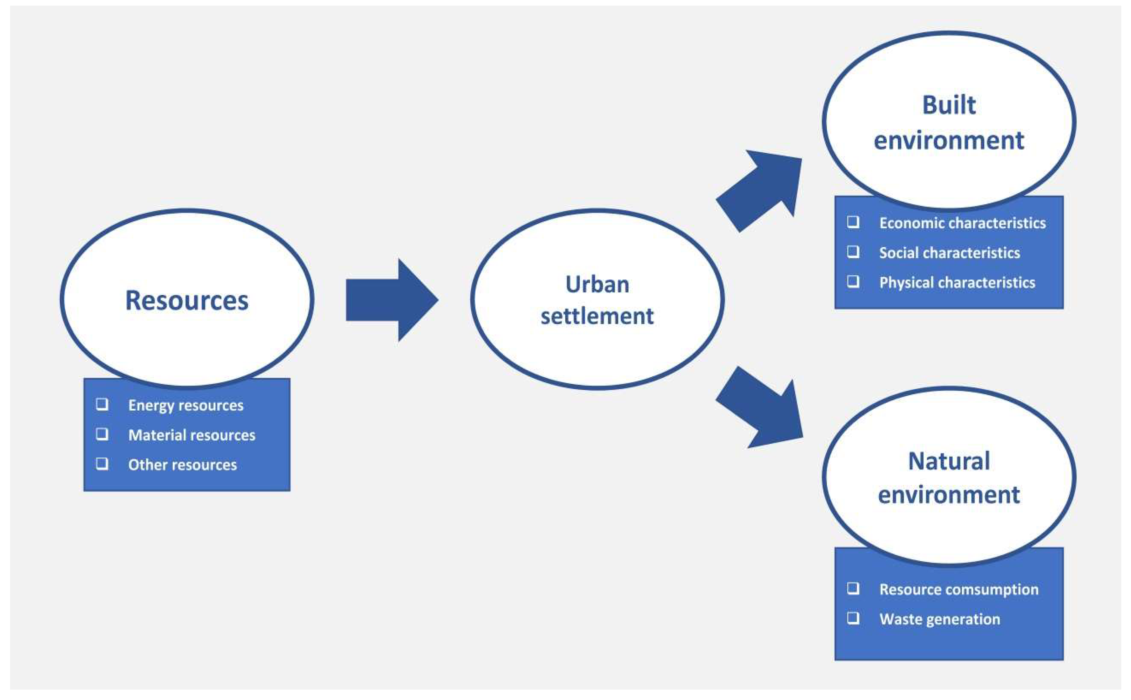
Newman [24] has proposed the use of the extended metabolism model of the city for urban planning, which intended to describe how cities operate as dynamic systems and their implicit complexities. This model highlights the crucial role of the natural environment, in that it provides the material and energy resources necessary in order to obtain a series of economic, social and physical infrastructures that create numerous opportunities for residents’ liveability. However, the physical and biological processes used to obtain these infrastructures also imply a series of unwanted effects that will impact on other urban considerations, as well as on the environment itself, both in terms of the overconsumption of resources and waste generation.
The way urban systems work, outlined in Figure 1, reveals the conflict that may arise between cities’ degree of liveability and their sustainability. As a result, cities may offer a high level of liveability, albeit at the cost of environmental degradation [24]. For example, a city may be considered liveable due to considerable job opportunities and a high degree of economic activity. However, these apparent advantages may also have a negative impact on environmental conditions, such as excessive air pollution caused by traffic congestion. In this particular example, urban managers should implement public transport measures and more efficient transport infrastructures to avoid these effects. A negative environmental impact poses a real threat for cities’ capacity to maintain their level of liveability in the future. Given that cities should work to secure a sustainable liveability, some authors have addressed the various ways of improving liveability without undermining environmental sustainability [12,16]. However, these methods require a series of prior environmental considerations to add to the classic notion of liveability.
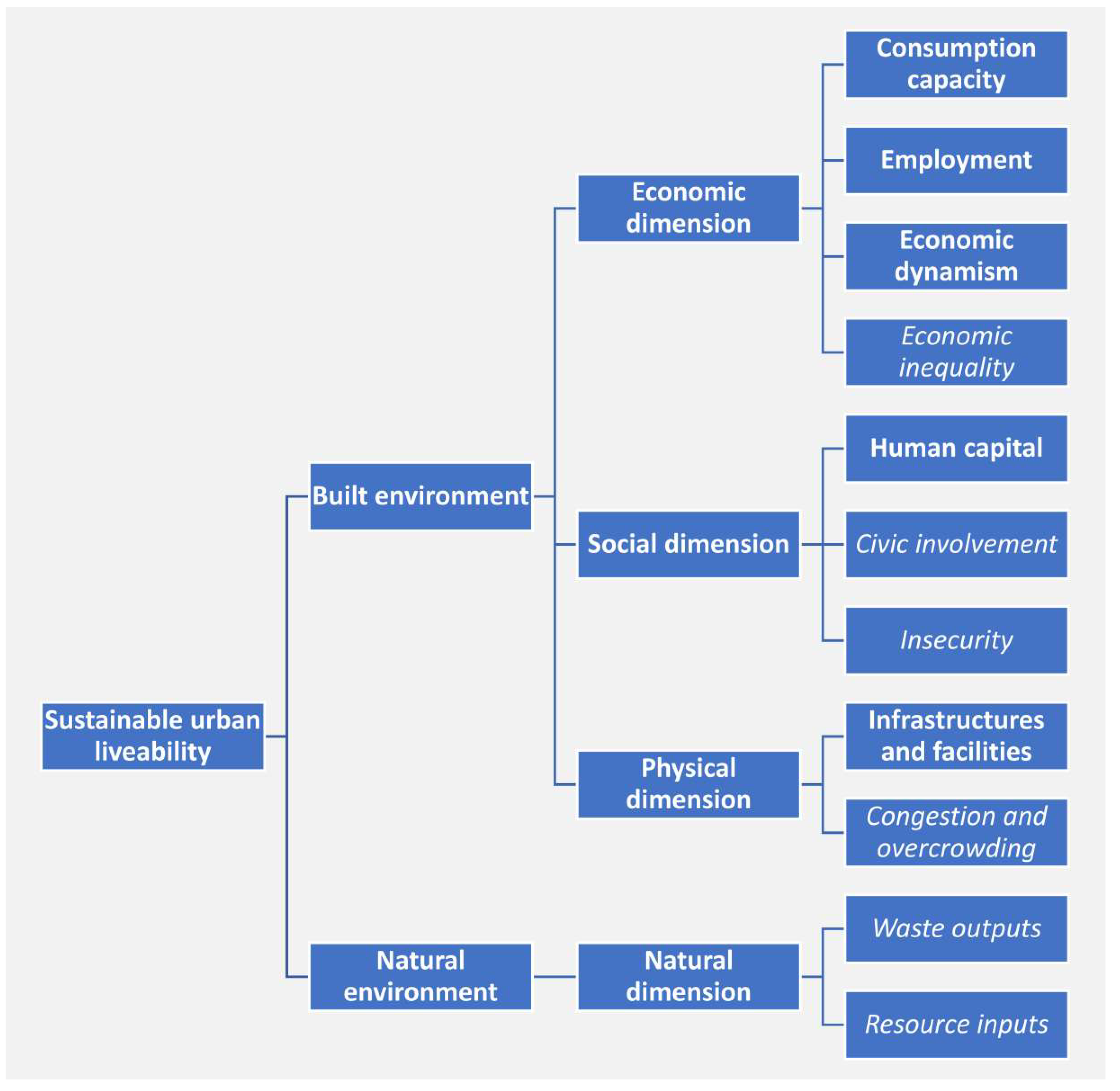
The concept of sustainable urban liveability posited in this article is based on the classic concept of urban liveability [15,16] applied to a long-term perspective. In this sense, we consider sustainable urban liveability to be the set of economic, social and physical attributes or characteristics of a certain urban area, which, when improved without deteriorating the environmental conditions, will have a positive impact on residents’ quality of life. Environmental sustainability is important in order to maintain liveability for future generations. Cities should therefore be capable of achieving this degree of liveability, whilst at the same time guaranteeing a minimum number of environmental conditions in terms of resource consumption and waste generation.
The concept of sustainable urban liveability is complex in that it comprises multiple dimensions. It should therefore be centred on the analysis of two groups of considerations, which correspond to the two environments that make up an urban system: the built environment and the natural environment.
The built environment refers to those elements created by humans and which have a greater presence in cities. In accordance with Newman’s model [24], liveability, based on the short-term approach, is associated with the combination of these elements. Regarding the classification of the elements that comprise the built environment and which determine the short term liveability of an urban area, literature has failed to reach a consensus beyond three broad areas: economic, social and physical [26,27]. As for the aspects included in each, urban agglomeration and city-based processes may have a positive impact (city effect) or a negative one (urban overload) [28].
The economic dimension of the built environment refers to the city as a center of economic activity, considering specific aspects related to individual urban conditions [29]. Literature in this area considers that the agglomeration of people has a positive impact on certain aspects such as consumption capacity [30,31,32], employment [30,33] and economic activity [28,30,34,35]. In contrast, cities can impact negatively on other aspects of liveability in this dimension, such as economic inequality [36,37], which tends to be higher than that experienced in other types of territory.
The social dimension provides a support network enabling urban residents to communicate with one another and take part in community life [26]. The high concentration of urban residents and activity levels have a positive impact on human capital [32,38]. However, urban agglomeration would appear to have an adverse effect on crucial social issues such as civic involvement in cooperation and volunteer networks [39,40] or citizen security [41,42].
The physical environment supports coexistence and provides a setting for urban residents [26]. There is a considerable degree of consensus regarding the twofold impact of agglomeration and processes on the physical environment of urban areas [28,31,43]. On the one hand, the density of urban populations is propitious for a series of infrastructures and education, health, transport and leisure services, which will have a positive impact on urban liveability. However, this same density has also led to the emergence and aggravation of problems such as the lack of housing and green areas, as well as traffic congestion.
In turn, the natural environment refers to the biological characteristics of nature. They play a key role in urban systems in two essential ways: firstly, the natural environment provides the raw materials and energy resources necessary for urban systems, and secondly, it assimilates the waste generated as a result of the processes these systems require. It is therefore clear that the agglomeration of people and activities in cities will have an adverse impact on the natural environment [44]. This impact consists essentially of the overconsumption of natural resources and an increase in the amount of waste generated.
A conceptual model for the two types of dimensions of the built and natural environment is provided in Figure 2. It illustrates various dimensions and sub-dimensions included in the sustainable urban liveability concept. As can be observed, the conceptual model attempts to differentiate between those sub-dimensions on which urban agglomeration has a positive impact (in bold) and those on which the impact is negative (in italics).
Given that sustainable urban liveability is a multi-dimensional and abstract concept, it must be estimated rather than measured directly. The composite indicator methodology applied in this case is highly appropriate for estimating such concepts. It is based on an approach to the various dimensions included in the concept through the application of one or various empirical variables known as “partial indicators.” The partial indicators that are representative of each dimension are weighted and aggregated in a single concept measurement known as a composite indicator [45] (for further information regarding the advantages and disadvantages of composite indicator methodology, see Nardo et al. [46]).
As occurs with all multidimensional concepts, no single dimension alone can guarantee a city’s liveability. Moreover, given that the objective is to ensure that the current situation will not compromise future liveability, positive performance in economic, social or physical dimensions would be pointless without compliance with a series of minimum environmental standards that are capable of guaranteeing that the level of urban liveability achieved can be sustained in the long term.
In order to comply with the theoretical requirements provided, an aggregation technique is needed that will prevent positive outcomes for the built environment from offsetting the poor results obtained in the partial indicators of the natural environment.
3. Materials and Methods
3.1. The Goal Programming Based Approach to Composite Indicator Construction
The technique employed in the construction of the sustainable urban liveability composite indicator is based on goal programming, which originated in the field of operational research [47,48,49]. Following earlier research conducted by Díaz-Balteiro and Romero [50], the goal concept appears for the first time in the construction of composite indicators in an article by Blancas et al. [23], which attempted to estimate the sustainability of tourist destinations. This same technique was later applied to other research projects [51,52,53,54,55,56,57].
In order to illustrate how goal programming works in the context of the construction of composite indicators, let us suppose that a series of N units (e.g., cities) are to be evaluated by means of M initial indicators. In line with their improvement direction, we have considered two types of indicators: positive ones, or the more the better, and negative ones, or the fewer the better. In this sense, we consider the existence of L positive indicators and K negative ones, whereby L + K = M. The variable Xil+ denotes the value of positive indicator l for unit i (l = 1, 2, …, L) and Xik− represents the value of negative indicator k for unit i (k = 1, 2, …, K).
An aspiration level is determined for each of the M indicators, representing an acceptable level of achievement (The aspiration level is exogenous to the model. These levels must be determined in accordance with external references, such as regulatory standards, determined by experts in the field or based on internal references as in the case of action objectives for the units evaluated. Nevertheless, it is often necessary to resort to alternative criteria [28], such as the use of empirically obtained levels (average values, minimum values or those obtained by benchmarking units). Although the use of these empirical levels implies acceptance of the status quo [58], this is an extremely common practice in the field of urban planning and management.). The value μl+ would be the aspiration level for positive indicator l and μk− would refer to the aspiration level for negative indicator k. Associated with each indicator and aspiration level, we can define a goal using the deviation variables denoted as n, in the case of negative ones, and p in that of positive ones. These deviations represent the difference between the value of an indicator and its corresponding aspiration level, so that the interpretation of such varies according to the type of indicator involved. Consequently, in the case of a positive partial indicator Xil+, the variable nil+ would express a weakness in this indicator, while pil+ would be the desired variable, since it would indicate a strength in this unit. As a result, the goals would be formulated as:
Xil+ + nil+ − pil+ = μl+, where nil+, pil+ ≥ 0; nil+. pil+ = 0, ∀l l = 1, 2, ..., L
In the case of a negative partial indicator Xik−, the variable pik− would be interpreted as a weakness in this indicator, while nik− would reflect a strength, representing the desired variable.
Xik− + nik− − pik− = μk−, where nik−, pij− ≥ 0; nik−. pik− = 0, ∀k k = 1, 2, …, K
Considering that the desirability of deviations depends on the positive/negative sign of the partial indicator, their interpretation may lead to confusion. Desirable deviations or strengths are therefore denoted as Sim. These variables would be positive deviations pil+, in the case of positive indicators, and negative deviations nik−, in the case of negative indicators. In turn, Wim denotes undesirable deviations or weaknesses, namely negative deviations nil+ when the indicator is positive, and positive deviations pik− when the indicator is negative. Moreover, considering that partial indicators may be measured on different scales, the deviation variables might not be comparable. They must therefore be expressed in relative terms, in other words as a percentage of their respective aspiration levels.
These deviation variables expressing strengths and weaknesses may be aggregated in a composite indicator to evaluate the performance of each unit considered in comparison with the predetermined aspiration levels. The use of this technique when constructing composite indicators holds numerous advantages over other statistical techniques; for instance, it does not require a sufficient difference between the number of units for analysis and the number of partial indicators employed in order to guarantee discrimination capacity [23], or the prior standardisation of the partial indicators for aggregation [50].
In addition, one of the greatest advantages of goal programming aggregation is that it is possible to consider the compensation or non-compensation of the deviation variables for each partial indicator. As a result, this technique is suitable for application both in contexts where full compensation between the strengths and weaknesses of the units evaluated could be recommendable, and in those where, from a theoretical perspective, the weaknesses a unit displays in certain indicators or dimensions cannot be compensated by strengths in others [23].
3.2. A Proposal for a Sustainable Urban Liveability Index (SULI): the Case of Spain
The goal programming-based aggregation technique described in the previous section will be used in the proposal for a composite index that will allow for the estimation of sustainable urban liveability. This technique will enable us to aggregate the various dimensions of sustainable urban liveability into a single measurement, whilst complying with the definition and theoretical framework of this concept. In this sense, goal programming-based aggregation allows for the non-compensation of the weaknesses of the natural environment for the strengths of the built environment in the case of cities that fail to meet minimum environmental aspiration levels. The construction of the sustainable urban liveability composite index is divided into two phases.
The initial phase consists of the analysis of the deviation variables (strengths and weaknesses) obtained for the J partial indicators of the natural environment for each city i. If a city displays any weakness in these partial indicators, it will be eliminated from the analysis as the minimum environmental standards have not been verified. This is to ensure that a city does not reach a current high degree of liveability at the expense of the overconsumption of resources and the degradation of the environment. However, the model proposed here does imply the possibility of classifying the cities that fail to meet these requirements by means of the indicator Ri. The indicator Ri can be defined as the sum of the weighted relative weaknesses in environmental indicators, divided between the sum of the weighting of said indicators. Consequently, Ri provides information of considerable use for cities that fail to meet the minimum environmental standards, enabling them to determine the percentage of non-compliance regarding the aspiration levels of these indicators.
Once the cities that fail to meet the minimum environmental standards have been identified, the next stage consists of constructing the urban liveability composite indicator for those cities that have no weaknesses in any of the natural environment dimensions. Unlike the previous phase, any weaknesses in the built environment indicators may be compensated by their strengths in other dimensions. The sustainable urban liveability composite index is therefore constructed as a lineal aggregate of strengths and weaknesses in previously weighted relative terms. The composite indicator may adopt positive values in the case of certain cities and negative ones in others. The index value will be positive, provided that the city has more strengths than weaknesses, and will be negative when the weaknesses exceed the strengths. In this sense, the higher a city’s composite index, the greater the degree of liveability it offers its residents.
The sustainable urban liveability composite index proposed in this article has a key advantage over other indicators presented to date; namely that it guarantees that the degree of liveability not only takes into account current levels, but also cities’ capacity to sustain these levels over time. Another major advantage of this proposal is its outstanding utility for urban planning and management; presenting indicators as deviation variables simplifies the process of identifying the strengths and weaknesses of each city.
The sustainable urban liveability composite index proposed here is applicable to all urban contexts in developed countries. However, in order to test the validity of our model, it was applied to a group of 58 Spanish cities. The initial idea was to analyse Spain´s 80 most important cities, not only in terms of population (cities with a minimum size of 100,000 inhabitants), but also including provincial and autonomous community capitals, which, despite their lower numbers of residents, play a relevant role within the urban system as centres for policy making and the provision of services at a regional level [59]. However, difficulties in obtaining data for certain partial indicators forced us to exclude 22 of these cities from our analysis (the following cities were excluded due to the lack of available data: Alcobendas, Alcorcón, Ávila, Cartagena, Cuenca, Dos Hermanas, Elche, Huesca, Lugo, Mérida, Móstoles, Parla, Pontevedra, Reus, San Cristóbal de la Laguna, Segovia, Soria, Telde, Terrassa, Teruel, Torrejón de Ardoz and Vigo).
The first stage in applying the composite index to the case of Spain involved selecting the partial indicators that represent each of the dimensions included in the theoretical framework for sustainable urban liveability. The starting point for this selection was a review of the indicators used in recent research in line with the objectives of this article [5,6,8,20,21,22,29,60,61,62,63,64,65,66]. Table 1 shows the final selection of partial indicators used to estimate the sustainable urban liveability composite index of Spanish cities, as well as their sign and the database they were obtained from and the year they refer to.
Regarding the partial indicators used, the lack of available data in terms of urban breakdown prevented the evaluation of the sub-dimension for economic inequality included in the theoretical framework. A cost of living indicator could not be included, and therefore the sub-dimension for “consumption capacity” was estimated using an income level indicator only. Likewise, an improved approach of the dimensions of natural environment requires the use of other major indicators such as the average concentration of NO2, the equivalent CO2 or water pollution. Unfortunately, data for these indicators were not available on a city scale. This lack of data has also prevented the use of partial indicators that in theory were considered ideal, requiring the use of alternatives. This was the case of the education infrastructures sub-dimension, where in the light of the lack of data, such as the number of places offered in state education centres, we were forced to resort to the use of a proxy variable, namely the number of reading/study spaces in public libraries.
The characteristics of the partial indicators in accordance with their descriptive statistics (mean value, standard deviation, maximum and minimum values) in the cities included in the study as well as the aspiration levels for each partial indicator are presented in Table 2 and Table 3. The corresponding analysis of the partial indicators reveals an average correlation of 0.236.
As the various partial indicators were to be used to construct a composite indicator, it was important to determine their internal coherence by means of some form of multivariate analysis technique. Cronbach’s Alpha [67], used mainly as an estimate of internal consistency of items in a model or survey [68], also allows for the assessment of how well a set of items (in our terminology individual indicators) measures a single uni-dimensional object [46]. In this case the value obtained for the Cronbach’s Alpha based on standardized items was 0.638. Nunnally [69] suggests 0.7 as an acceptable reliability threshold, while others are more lenient and suggest 0.6 [46].
As discussed above, both the aspiration levels and the weighting for each of the partial indicators are exogenous to the model. In other words, goal programming-based aggregation enables urban planners to determine both variables in accordance with the real situation, as well as the needs and objectives of the cities under analysis.
When determining the aspiration levels of this proposal, external references were detected for the three natural environment indicators. In this sense, the aspiration level determined for the “average annual concentration of PM10,” is the maximum value of 40 mcg/m3 stipulated in European Directive 2008/50/CE of the European Parliament and of the Council of 21 May 2008. The aspiration levels selected for the indicators “generation of solid waste per inhabitant” (1.4 kg of waste per inhabitant per day), and “domestic electricity consumption per inhabitant” (10 MWh per person per year) were based on the maximum desirable values established in the Municipal Sustainable Indicators System drawn up by the Spanish Ministry of the Environment and Rural and Marine Affairs [70]. As for the built environment indicators, the lack of external references meant that the aspiration level had to be set empirically, as has occurred with previous research projects [23,50]. The decision was taken to use the value corresponding to the arithmetic mean of the observations for the 58 cities analysed. The specific aspiration levels for the 15 partial indicators are presented in Table 2 and Table 3.
In the specific case of the application of the composite indicator to Spanish cities, and as discussed by a number of authors, the choice of weighting system was conditioned by the need for a balance between urban environment dimensions [26]. It is for this reason that the decision was taken to assign equal weighting to all four dimensions of sustainable urban liveability: economic, social, physical and natural. This weighting would likewise be distributed equally between the partial indicators included in each dimension in order to ensure that weighting patterns were not attributed to specific urban interests.
4. Results and Discussion
Considering that the aspiration levels for each of the partial indicators could be an issue for debate, this also posed the question of the model’s uncertainty. An uncertainty and sensitivity analysis was therefore conducted centred on these aspiration levels, and alternative aspiration levels were selected for the partial indicators, resulting in 12,754,584 possible combinations. A full analysis of all these combinations would prove extremely complicated in computational terms, and therefore a statistically representative sample was selected, comprising 16,566 aspiration level combinations, with a 99% confidence interval and 1% sample error. The SULI was therefore estimated for each aspiration level combination, resulting in 16,566 values for each of the cities analysed, generating an empirical probability distribution for the composite index. The results of the uncertainty analysis reveal a high degree of consistency with the principal results obtained for the model, both in terms of the SULI values and the classification of the various cities. Furthermore, the sensitivity analysis indicated that the aspiration levels with the greatest impact on the results are the waste indicator and to a lesser extent the aspiration level of the air quality indicator, whilst the rest of the aspirations levels have practically no impact on the results.
The initial phase of the results analysis involved identifying those cities that failed to meet the minimum environmental requirements. All 58 Spanish cities met the minimum acceptable standard of air quality, although 14 cities (Table 4) failed to meet the minimum acceptable standard for waste (WAS) and one also failed to meet the minimum standard for electricity consumption (ELE). Analysing the weaknesses (Table 4) allowed us to consider the limits exceeded for each environmental indicator. The performances of these cities on the Ri index are also reported (Table 4). In this regard, the values of this index reveal a low degree of non-compliance; the only exception in this sense is Marbella, with an Ri index of more than 15%.
After excluding those cities that could not be considered environmentally sustainable, the SULI was applied to the remaining 44 cities. Table 5 indicates that 37 cities obtained a positive value for the SULI, indicating that in net terms, their strengths exceed their weaknesses, whilst the other 7 cities showed more weaknesses than strengths.
The SULI values (Ri values and the SULI indicators for all the cities analysed are provided as Supplementary Materials) allow for the classification of the cities based on their urban liveability. Pamplona obtained the highest SULI value (0.329), positioning it as the most liveable of the cities analysed, followed by the Basque city of Donostia (San Sebastian), which obtained a composite index value of 0.321. The cities of Cáceres and Ciudad Real also performed well, with SULI values of around 0.2, whilst Burgos, Ourense, Vitoria, Zamora and Salamanca produced values of between 0.13 and 0.17. At the opposite end of the classification we found a number of Andalusian cities, such as Algeciras, Huelva or Jerez de la Frontera, as well as several Catalonian cities, including Santa Coloma de Gramenet, L’Hospitalet de Llobregat or Badalona, which all obtained negative liveability index values.
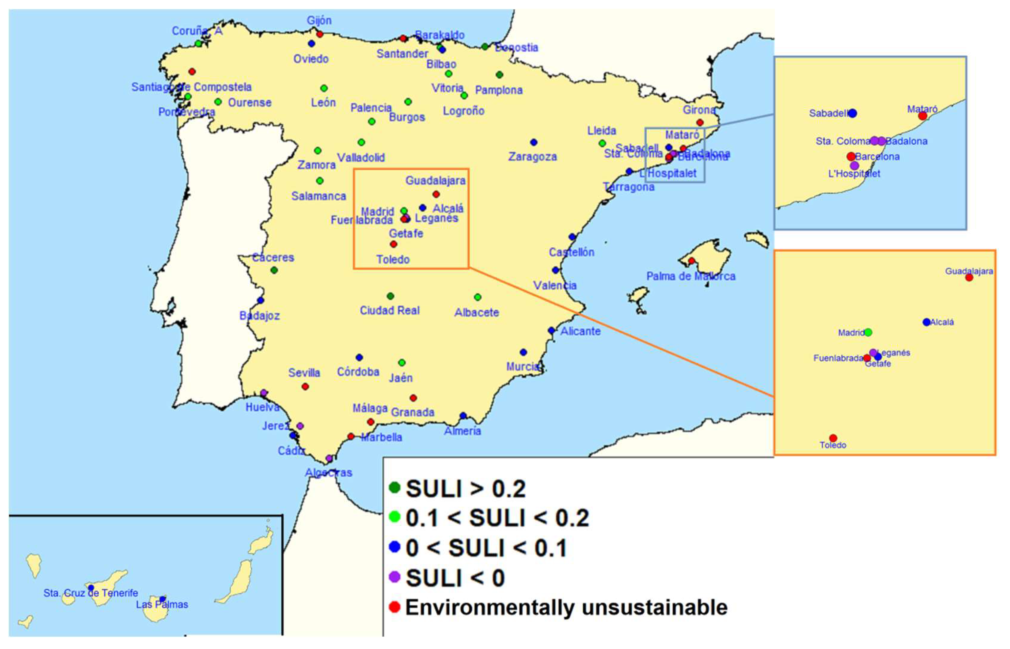
The geographical distribution of the results obtained is illustrated in Figure 3, revealing that no particular geographical pattern can be attributed to the cities that fail to meet the aspiration levels of the natural environment indicators. However, it is worthy of note that 7 of these 15 cities are some of the most popular urban tourism destinations in Spain according their number of visitants per inhabitant: Barcelona, Granada, Marbella, Palma de Mallorca, Santiago de Compostela, Sevilla or Toledo. This information should act as a warning sign for their managers, indicating the need for additional measures to promote sustainable tourism [71,72].
The 44 remaining cities that exceeded these aspiration levels of environmental indicators follow a geographical pattern (for a better understanding the of Spain’s regional character, a map featuring the autonomous communities classified by geographic location (northern, central and southern) as well as a table with the cities analysed classified by their geographical location have been included as Supplementary Material). Indeed, cities that had composite indicator values of more than 0.1 are located mainly in the north and the centre of the country, in particular in the regions of Galicia, the Basque Country, Castile and Leon and Navarre. In contrast, cities obtaining negative index values and therefore offer lower levels of liveability are concentrated mainly in western Andalusia and the province of Barcelona. This way, the average SULI value for cities located in the north and in the centre of Spain is approximately 0.1 in both cases, compared with the far lower average value of 0.02 for cities located in the south. These results are in line with other studies [73,74], which revealed a higher quality of life in municipalities located in northern and central Spain, whilst the lowest levels were to be found in the south, specifically in Andalusia, Murcia and the Valencian Community.
Identifying strengths and weaknesses in specific dimensions may be useful when implementing polices aimed at improving urban liveability levels. By means of an example, Table 6 lists the relative deviation variables (strengths and weaknesses) in percentage terms for those cities that scored lowest in terms of sustainable urban liveability.
From the perspective of urban planners, the dimensions with the highest concentration of serious weaknesses could require more urgent action. In the case of the five cities analysed, these weaknesses were including in the partial indicators for green spaces (GRE) and leisure infrastructures (CIN). However, despite their overall poor performance, some of these cities registered major strengths that urban planners could and should take into consideration when designing promotional strategies for the city. Although all five cities present strengths for the partial indicator relating to electricity consumption, the strengths of four (Santa Coloma de Gramenet, L’ Hospitalet de Llobregat, Algeciras and Jerez de la Frontera) are particularly worthy of note due to their magnitude. In addition, the two Catalonian cities (Santa Coloma de Gramenet and L’Hospitalet de Llobregat) also present significant strengths for the partial indicator transport infrastructures. Similar analyses for any of the cities included in the study would provide planners with useful information, allowing for the identification of relatively weaker partial indicators, even in the case of the top performing cities.
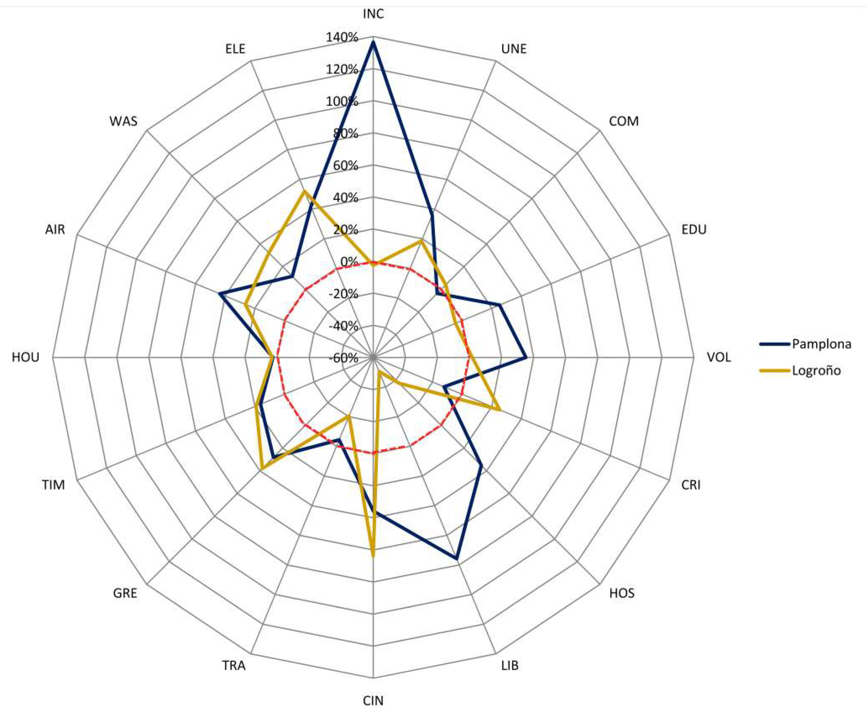
Goal programming aggregation also allowed for a benchmarking analysis of cities which, despite sharing similar morphological and functional characteristics, obtained very different results in terms of their sustainable urban liveability. In this sense, benchmarking enables cities to “learn from one another”. By way of an example, Figure 4 shows the cases of the cities of Pamplona and Logroño based on the comparison of their deviation variables.
Both cities are located in the north of Spain, have similar populations and are classified as transnational/national in accordance with the functions defined by European Observation Network for Territorial Development and Cohesion (ESPON) [75]. Yet despite their similarities, there are significant differences in terms of their performance in sustainable urban liveability. Whilst Pamplona tops the ranking, with a SULI value of 0.329, Logroño obtained a composite index value of 0.132, positioning it in eleventh place. On the basis of this information, Pamplona could be considered a liveability benchmark for Logroño.
Pamplona scores considerably higher than Logroño in many of the partial indicators for sustainable urban liveability included in the study. In this sense, Logroño has considerable room for improvement in areas such as education infrastructures (EDU) and income levels (INC) in particular. However, this latter partial indicator is not the city’s greatest weakness in absolute terms, as it falls only slightly short of the aspiration level. As a result, Logroño’s urban planners should focus on improving these specific aspects in order to improve the city’s relative position. It must also be stated that Logroño performs significantly better than Pamplona in terms of citizen security (CRI). In relative terms, urban planners should interpret this as an indication of the effectiveness of the policies applied in this specific area.
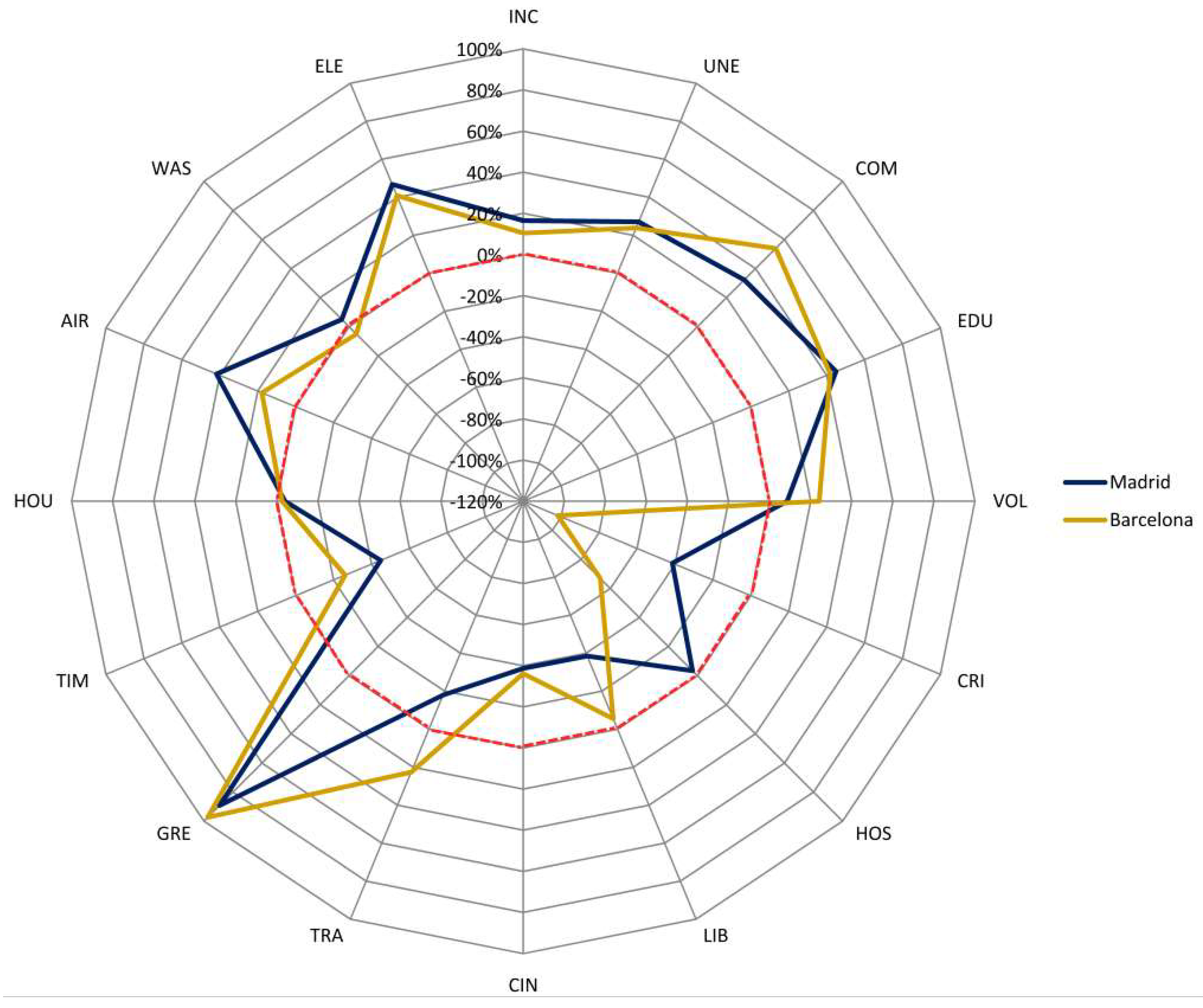
A benchmarking analysis may also be carried out to compare an environmentally non-sustainable city with an environmentally sustainable one. This could be the case of Madrid and Barcelona, Spain’s two most important cities (Figure 5). According to our model, Barcelona failed to meet the aspiration levels of the waste generation indicator and was therefore classified as environmentally unsustainable, whilst Madrid was classified as sustainable.
Since Barcelona and Madrid share similar morphological and functional characteristics, their performance in certain partial indicators differs only slightly. This is true in the case of the income (INC), unemployment (UNE), education infrastructures (EDU), green zones (GRE), housing (HOU) and electricity consumption (ELE) indicators, where both cities register strengths of similar importance, and for the leisure infrastructure indicators, where both cities almost present identical weaknesses. However, Barcelona performed worse than Madrid, not only in the environmental indicators, but also in others, as in the case of citizen security (CRI) and health infrastructures (HOS). Based on this information, urban managers of Barcelona should begin by addressing the problem of waste as it represents a threat to the liveability of future generations. Once this priority problem has been solved, attention should be focused on implementing measures to improve security and health infrastructures.
5. Conclusions
The main contribution of this article is to address an essential but rarely discussed issue, namely the limitations of the traditional approach to calculating quantitative measures of urban liveability that do not consider its environmental sustainability. In this sense, this paper presents two key outcomes. First, it introduces a concept of sustainable urban liveability defined as the set of environmental, social and economic characteristics of a specific urban area, which once improved, will impact positively on residents’ quality of life, without compromising its future sustainability. In this sense, securing sustainable urban liveability must depend on compliance with a set of minimum environmental requirements in terms of resource consumption and environmental degradation. Second, it posits an evaluation instrument based on a goal programming based index, preventing cities from scoring high levels of liveability at the expense of environmental degradation. In this sense, the proposed index allows for the non-compensation between partial indicators, and also provides highly useful information that can easily be interpreted by non-experts in this field, such as urban managers and planners.
Therefore, our research can contribute to enhancing (sustainable) urban liveability; improving cities’ attributes requires the design of instruments enabling urban planners to estimate existing sustainable living conditions as well as the effectiveness of actions carried out to attain more liveable and sustainable cities.
It is important to highlight the limitations of the study, partially related to the question of data availability. First, the selection of indicators in relation to environmental sustainability is currently rather narrow, due to the fact that this kind of data is rarely available, especially on a local scale. The shortage of local data not only makes it difficult to compare environmental performance among cities, but also excludes other key indicators that are crucial when estimating in terms of economic inequality or the cost of living. A further difficulty lies in the question of municipal boundaries, because although the available data refer always to the municipal level, the urban reality frequently extends beyond municipal boundaries, a complex issue for this kind of analysis. Finally, and because the scientific community has failed to reach a consensus regarding the aspiration levels for the built environment partial indicators, on this occasion we were forced to use aspiration levels obtained empirically for these indicators. In this context, more urban data and more frequent interaction with urban managers and planners when setting aspiration levels are needed in order to improve the instrument proposed.
In spite of these limitations, our research attempts to break away from the traditional short-term vision of liveability, indicating that the only way ahead in this sense implies compliance with a series of basic sustainability criteria. In order to further this notion, future research should address in greater depth the relationship between liveability and environmental sustainability in urban contexts. At all events, urban managers and planners should take this new approach to liveability into consideration, working to secure improvements to liveability conditions not only for the present, but also for the future. Faced with this challenge, the scientific community must provide urban managers and planners with the instruments necessary to put this new vision of liveability into practice.
Supplementary Materials
The following are available online at https://www.mdpi.com/2071-1050/11/1/86/s1, Figure S1: Geographical distribution of autonomous communities of Spain, Table S1: Cities and values of SULI and R.
Author Contributions
Conceptualization, B.V.A. and P.M.; Data curation, B.V.A.; Formal analysis, B.V.A.; Investigation, B.V.A. and P.M.; Methodology, B.V.A. and D.R.-G.; Project administration, P.M.; Resources, B.V.A.; Software, D.R.-G.; Supervision, P.M.; Validation, P.M.; Visualization, D.R.-G.; Writing—original draft, B.V.A.; Writing—review and editing, B.V.A., P.M. and D.R.-G.
Funding
This research received no external funding.
Conflicts of Interest
The authors declare no conflict of interest.
References
- European Commission. State of European Cities Report. Adding Value to the European Urban Audit; European Commission: Brussels, Belgium, 2007. [Google Scholar]
- UN-Habitat. State of the World´s Cities 2008–2009: Harmonious Cities; Earthscan: London, UK, 2008. [Google Scholar]
- Major Cities Unit. State of Australian Cities; Infrastructure Australia: Canberra, Australia, 2010. [Google Scholar]
- Ülengin, B.; Ülengin, F.; Güvenç, Ü. A multidimensional approach to urban quality of life: The case of Istanbul. Eur. J. Oper. Res. 2001, 130, 361–374. [Google Scholar] [CrossRef]
- Morais, P.; Camanho, A.S. Evaluation of performance of European cities with the aim to promote quality of life improvements. Omega 2011, 39, 398–409. [Google Scholar] [CrossRef] [Green Version]
- Morais, P.; Miguéis, V.L.; Camanho, A.S. Quality of life experienced by human capital: An assessment of European cities. Soc. Indic. Res. 2013, 110, 187–206. [Google Scholar] [CrossRef]
- Saitluanga, B.L. Spacial pattern of urban livability in Himalayan region: A case of Aizawl City, India. Soc. Indic. Res. 2014, 117, 541–559. [Google Scholar] [CrossRef]
- Arundel, J.; Lowe, M.; Hooper, P.; Roberts, R.; Rozek, J.; Higgs, C.; Giles-Corti, B. Creating Liveable Cities in Australia. Mapping Urban Policy Implementation and Evidence-Based National Liveability Indicators; Centre for Urban Research RMIT University: Melbourne, Australia, 2017. [Google Scholar]
- Godschalk, D.R. Land use planning challenges: Coping with conflicts in visions of sustainable development and livable communities. J. Am. Plan. Assoc. 2004, 70, 5–13. [Google Scholar] [CrossRef]
- Howley, P.; Scott, M.; Redmond, D. Sustainability versus liveability: An investigation of neighbourhood satisfaction. J. Environ. Plan. Manag. 2009, 52, 847–864. [Google Scholar] [CrossRef]
- Allen, T.F.H. Making livable sustainable systems unremarkable. Syst. Res. Behav. Sci. 2010, 27, 469–479. [Google Scholar] [CrossRef]
- Chazal, J. A systems approach to livability and sustainability: Defining terms and mapping reationships to link desires with ecological opportunities and constraints. Syst. Res. Behav. Sci. 2010, 27, 585–597. [Google Scholar] [CrossRef]
- Lewis, N.M.; Donald, B. A new rubric for ‘creative city’ potential in Canada’s smaller cities. Urban Stud. 2010, 47, 29–54. [Google Scholar] [CrossRef]
- Ruth, M.; Franklin, R.S. Livability for all? Conceptual limits and practical implications. Appl. Geogr. 2014, 49, 18–23. [Google Scholar] [CrossRef] [Green Version]
- Gough, M.Z. Reconciling livability and sustainability: Conceptual and practical implications for planning. J. Plan. Educ. Res. 2015, 35, 145–160. [Google Scholar] [CrossRef]
- Newton, P.W. Liveable and sustainable? Socio-technical challenges for twenty-first-century cities. J. Urban Technol. 2012, 19, 81–102. [Google Scholar] [CrossRef]
- Ekins, P.; Simon, S.; Deutsch, L.; Folke, C.; De Groot, R. A framework for the practical application of the concepts of critical natural capital and strong sustainability. Ecol. Econ. 2003, 44, 165–185. [Google Scholar] [CrossRef] [Green Version]
- Dietz, S.; Neumayer, E. Weak and strong sustainability in the SEEA: Concepts and measurement. Ecol. Econ. 2007, 61, 617–626. [Google Scholar] [CrossRef] [Green Version]
- Bithas, K.P.; Christofakis, M. Environmentally Sustainable Cities. Critical Review and Operational Conditions. Sustain. Dev. 2006, 14, 177–189. [Google Scholar] [CrossRef]
- Mori, K.; Fujii, T.; Yamashita, T.; Mimura, Y.; Uchiyama, Y.; Hayashi, K. Visualization of a City Sustainability Index (CSI): Towards transdisciplinary approaches involving multiple stakeholders. Sustainability 2015, 7, 12402–12424. [Google Scholar] [CrossRef]
- Higgins, P.; Campanera, J.M. (Sustainable) quality of life in English city locations. Cities 2011, 28, 290–299. [Google Scholar] [CrossRef]
- Zanella, A.; Camanho, A.S.; Dias, T.G. The assessment of cities’ livability integrating human wellbeing and environmental impact. Ann. Oper. Res. 2015, 226, 695–726. [Google Scholar] [CrossRef]
- Blancas, F.J.; Caballero, R.; González, M.; Lozano-Oyola, M.; Pérez, F. Goal programming synthetic indicators: An application for sustainable tourism in Andalusian coastal counties. Ecol. Econ. 2010, 69, 2158–2172. [Google Scholar] [CrossRef]
- Jones, C.; Newsome, D. Perth (Australia) as one of the world’s most liveable cities: A perspective on society, sustainability and environment. Int. J. Tour. Cities 2015, 1, 18–35. [Google Scholar] [CrossRef]
- Newman, P.W.G. Sustainability and cities: Extending the metabolism model. Landsc. Urban Plan. 1999, 44, 219–226. [Google Scholar] [CrossRef]
- Shafer, C.S.; Lee, B.K.; Turner, S. A tale of three greenway trails: User perceptions related to quality of life. Landsc. Urban Plan. 2000, 49, 163–178. [Google Scholar] [CrossRef]
- Das, D. Urban Quality of Life: A Case Study of Guwahati. Soc. Indic. Res. 2008, 88, 297–310. [Google Scholar] [CrossRef]
- Cicerchia, A. Measures of optimal centrality: Indicators of city effect and urban overloadin. Soc. Indic. Res. 1999, 46, 273–299. [Google Scholar] [CrossRef]
- Santos, L.D.; Martins, I. Monitoring urban quality of life: The Porto experience. Soc. Indic. Res. 2007, 80, 411–425. [Google Scholar] [CrossRef]
- Fujita, M.; Thisse, J.F. Economics of Agglomeration. J. Jpn. Int. Econ. 1996, 10, 339–378. [Google Scholar] [CrossRef]
- Glaeser, E.L.; Kolko, J.; Saiz, A. Consumer city. J. Econ. Geogr. 2001, 1, 27–50. [Google Scholar] [CrossRef]
- Glaeser, E.L.; Mare, D.C. Cities and Skills. J. Labor Econ. 2001, 19, 316–342. [Google Scholar] [CrossRef]
- Duranton, G.; Puga, D. Micro-Foundations of Urban Agglomeration Economies; National Bureau of Economic Research Working Papers; National Bureau of Economic Research: Cambridge, MA, USA, 2004; Volume 9931. [Google Scholar]
- Puga, D. The magnitude and causes of agglomeration economies. J. Reg. Sci. 2010, 50, 203–219. [Google Scholar] [CrossRef]
- Rodríguez-Pose, A. The revenge of the places that don’t matter (and what to do about it). Camb. J. Reg. Econ. Soc. 2018, 11, 189–209. [Google Scholar] [CrossRef]
- Wheeler, C. Cities, skills and inequality. Growth Chang. 2005, 36, 329–353. [Google Scholar] [CrossRef]
- Glaeser, E.L.; Ressenger, M.; Tobio, K. Urban Inequality; NBER Working Paper Series 14419; National Bureau of Economic Research: Cambridge, MA, USA, 2008. [Google Scholar]
- Abel, J.R.; Gabe, T.M.; Stolarick, K. Skills across the urban-rural hierarchy. Growth Chang. 2014, 45, 499–517. [Google Scholar] [CrossRef]
- Hughes, P.; Bellamy, J.; Black, A. Social trust: Locally and across Australia. Third Sect. Rev. 1999, 5, 5–24. [Google Scholar]
- Ziersch, A.M.; Baum, F.; Darmawan, I.G.N.; Kavanagh, A.M.; Bentley, R.J. Social capital and health in rural and urban communities in South Australia. Aust. N Z J. Public Health 2009, 33, 7–16. [Google Scholar] [CrossRef] [PubMed] [Green Version]
- Cullen, J.B.; Levitt, S.D. Crime, urban flight, and the consequences for cities. Rev. Econ. Stat. 1999, 81, 159–169. [Google Scholar] [CrossRef]
- Glaeser, E.L.; Sacerdote, B. Why is there more crime in cities? J. Political Econ. 1999, 107, S225–S258. [Google Scholar] [CrossRef]
- Archibugi, F. City effect and urban overload as a program indicators of the regional policy. Soc. Indic. Res. 2001, 54, 209–230. [Google Scholar] [CrossRef]
- Berry, B.J.L. Urbanization. In The Earth as Transformed by Human Action: Global and Regional Changes in the Biosphere over the Past 300 Years; Turner, B.L., Clark, W.C., Kates, R.W., Richards, J.F., Mathews, J.T., Meyer, W.B., Eds.; Cambridge University Press: Cambridge, UK, 1990. [Google Scholar]
- Saisana, M.; Tarantola, S. State-of-the-art report on current methodologies and practices for composite indicator development; European Commission, Joint Research Centre: Ispra, Italy, 2002. [Google Scholar]
- Nardo, M.; Saisana, M.; Saltelli, A.; Tarantola, S.; Hoffman, A.; Giovannini, E. Handbook on Constructing Composite Indicators: Methodology and User Guide; Organisation for Economic Co-Operation and Development: Paris, France, 2008. [Google Scholar]
- Charnes, A.; Cooper, W. Management Models and Industrial Applications of Linear Programming; Wiley: New York, NY, USA, 1961. [Google Scholar]
- Lee, S.M. Goal Programming for Decision Analysis; Auerbach: Philadelphia, PA, USA, 1972. [Google Scholar]
- Ignizio, J.P. Goal Programming and Extensions; Lexington Books: Lexington, UK, 1976. [Google Scholar]
- Díaz-Balteiro, L.; Romero, C. Sustainability of forest management plans: A discrete goal programming approach. J. Environ. Manag. 2004, 71, 351–359. [Google Scholar] [CrossRef]
- Lozano-Oyola, M.; Blancas, F.J.; González, M.; Caballero, R. Sustainable tourism indicators as planning tools in cultural destinations. Ecol. Indic. 2012, 18, 659–675. [Google Scholar] [CrossRef]
- Blancas, F.J.; Lozano-Oyola, M.; González, M. A European Sustainable Tourism Labels proposal using a composite indicator. Environ. Impact Assess. Rev. 2015, 54, 39–54. [Google Scholar] [CrossRef]
- Molinos-Senante, M.; Marques, R.C.; Pérez, F.; Gómez, T.; Sala-Garrido, R.; Caballero, R. Assessing the sustainability of water companies: A synthetic indicator approach. Ecol. Indic. 2016, 61, 577–587. [Google Scholar] [CrossRef]
- Pérez, V.; Hernández, A.; Guerrero, F.; León, M.A.; da Silva, C.L.; Caballero, R. Sustainability ranking for Cuban tourist destinations based on composite indexes. Soc. Indic. Res. 2016, 129, 425–444. [Google Scholar] [CrossRef]
- Blancas, F.J.; Lozano-Oyola, M.; González, M.; Caballero, R. A dynamic sustainable tourism evaluation using multiple benchmarks. J. Clean. Prod. 2018, 174, 1190–1203. [Google Scholar] [CrossRef]
- Cabello, J.M.; Navarro-Jurado, E.; Rodríguez, B.; Thiel-Ellul, D.; Ruiz, F. Dual weak-strong sustainability synthetic indicators using a double reference point scheme: The case of Andalucía, Spain. Oper. Res. 2018. Available online: https://link.springer.com/article/10.1007/s12351-018-0390-5 (accessed on 6 November 2018). [CrossRef]
- Valcárcel-Aguiar, B.; Murias, P. Evaluation and management of urban liveability: A goal programming based composite indicator. Soc. Indic. Res. 2018. Available online: https://link.springer.com/article/10.1007/s11205-018-1861-z (accessed on 6 November 2018). [CrossRef]
- Delion, H.; Irmen, E. National report on Germany. In The Integration of Cities into Their Regional Government: Toward a European Urban Systems Concept and Policy; Archibugi, F., Ed.; Planning Studies Centre: Rome, Italy, 1996. [Google Scholar]
- Bellet, C.; Llop, J.M. Miradas a otros espacios urbanos: Las ciudades intermedias. Scr. Nova Rev. Electron. Geogr. Cienc. Soc. 2004, 165, 1–8. [Google Scholar]
- Tanguay, G.A.; Rajaonson, J.; Lefebvre, J.-F.; Lanoie, P. Measuring the sustainability of cities: An analysis of the use of local indicators. Ecol. Indic. 2010, 10, 407–418. [Google Scholar] [CrossRef]
- Han, J.; Liang, H.; Hara, K.; Uwasu, M.; Dong, L. Quality of life in China’s largest city, Shanghai: A 20-year subjective and objective composite assessment. J. Clean. Prod. 2018, 173, 135–142. [Google Scholar] [CrossRef]
- Turcu, C. Re-thinking sustainability indicators: Local perspectives of urban sustainability. J. Environ. Plan. Manag. 2013, 56, 695–719. [Google Scholar] [CrossRef]
- Braulio-Gonzalo, M.; Bovea, M.D.; Ruá, M.J. Sustainability on the urban scale: Proposal of a structure of indicators for the Spanish context. Environ. Impact Assess. Rev. 2015, 53, 16–30. [Google Scholar] [CrossRef] [Green Version]
- Nissi, E.; Sarra, A. A measure of well-being across the Italian urban areas: An integrated DEA-entropy approach. Soc. Indic. Res. 2018, 136, 1183–1209. [Google Scholar] [CrossRef]
- Peach, N.D.; Petach, L.A. Development and quality of life in cities. Econ. Dev. Q. 2016, 30, 32–45. [Google Scholar] [CrossRef]
- Arbab, P. City Prosperity Inititative Index: Using AHP method to recalculate the weights of dimensions and sub-dimensions in reference to Tehran Metropolis. Eur. J. Sustain. Dev. 2017, 6, 289–301. [Google Scholar] [CrossRef]
- Cronbach, L.J. Coefficient alpha and the internal structure of tests. Psychometrika 1951, 16, 297–334. [Google Scholar] [CrossRef] [Green Version]
- Boscarino, J.A.; Figley, C.R.; Adams, R.E. Compassion Fatigue following the September 11 Terrorist Attacks: A Study of Secondary Trauma among New York City Social Workers. Int. J. Emerg. Ment. Health 2004, 6, 1–10. [Google Scholar]
- Nunnally, J. Psychometric Theory; McGraw-Hill: New York, NY, USA, 1978. [Google Scholar]
- Spanish Ministry of the Environment and Rural and Marine Affairs. Sistema Municipal de Indicadores de Sostenibilidad. IV Reunión del Grupo de Trabajo de Sostenibilidad de la Red de Redes de Desarrollo Local Sostenible. 2010. Available online: https://www.fomento.gob.es/recursos_mfom/pdf/82B973EA-5970-46F0-8AE6-65370D40A1F5/111505/SIST_MUNI_INDI_SOSTE_tcm7177732.pdf (accessed on 21 December 2018).
- Murzyn-Kupisz, M. Cultural, economic and social sustainability of heritage tourism: Issues and challenges. Econ. Environ. Stud. 2012, 12, 113–133. [Google Scholar]
- Ghafari, F.; Lahmian, R. The role of tourism industry in the management of sustainable urban development (Case study: Coastal cities of Mazandaran province). Int. J. Hum. Cult. Stud. 2016, 1381–1391. Available online: https://www.ijhcs.com/index.php/ijhcs/article/viewFile/1254/1116 (accessed on 21 December 2018).
- González, E.; Cárcaba, A.; Ventura, J. The Importance of the Geographic Level of Analysis in the Assessment of the Quality of Life: The Case of Spain. Soc. Indic. Res. 2011, 102, 209–228. [Google Scholar] [CrossRef]
- González, E.; Cárcaba, A.; Ventura, J. Weight constrained DEA measurement of the quality of life in Spanish municipalities in 2011. Soc. Indic. Res. 2018, 136, 1157–1182. [Google Scholar] [CrossRef] [PubMed]
- ESPON. The Role, Specific Situation and Potentials of Urban Areas as Nodes in a Polycentric Development; Third Interim Report; ESPON: Luxembourg, 2003. [Google Scholar]
Figure 1.
How an urban system works. Source: authors’ own based on Newman [25].
Figure 1.
How an urban system works. Source: authors’ own based on Newman [25].

Figure 2.
Conceptual framework of sustainable urban liveability.

Figure 3.
Geographical distribution of the results.

Figure 4.
Comparative analysis of relative deviation variables (expressed in percentages) for Pamplona and Logroño. The red line represents a relative deviation variable of 0%. Values above and below this level represent strengths and weaknesses respectively.
Figure 4.
Comparative analysis of relative deviation variables (expressed in percentages) for Pamplona and Logroño. The red line represents a relative deviation variable of 0%. Values above and below this level represent strengths and weaknesses respectively.

Figure 5.
Comparative analysis of relative deviation variables (expressed in percentages) for Madrid and Barcelona. The red line represents a relative deviation variable of 0%. Values above and below this level represent strengths and weaknesses respectively.
Figure 5.
Comparative analysis of relative deviation variables (expressed in percentages) for Madrid and Barcelona. The red line represents a relative deviation variable of 0%. Values above and below this level represent strengths and weaknesses respectively.


Table 1.
Partial indicators used in the application of the SULI in Spain.
| Sub-dimensions | Partial indicator | Abbreviation | Sign | Database | Year |
|---|---|---|---|---|---|
| Consumption capacity | Average net disposable income per household | INC | + | Urban indicators (Spanish National Statistics Office) | 2011 |
| Employment | Unemployment rate | UNE | − | Urban indicators (Spanish National Statistics Office) | 2011 |
| Economic dynamism | No. of companies per 1000 inhabitants | COM | + | Urban Audit (Eurostat) | 2011 |
| Human capital | Percentage of the population (25–64 years) with higher education per 1000 inhabitants | EDU | + | Urban indicators (Spanish National Statistics Office) | 2011 |
| Social capital | Percentage of the population that participates in volunteer work | VOL | + | Population and housing census (Spanish National Statistics Office | 2011 |
| Insecurity | No. of crimes and offenses per 1000 inhabitants | CRI | − | Criminality Statistics System (Spanish Ministry of the Interior) | 2013 |
| Infrastructures and services | No. of hospital beds per 1000 inhabitants | HOS | + | National Catalogue of Hospitals (Spanish Ministry of Health) | 2011 |
| Number of reading /study spaces in libraries per 1000 inhabitants | LIB | + | Public Library figures (Spanish Ministry of Education) | 2011 | |
| No. of cinema seats per 1000 inhabitants | CIN | + | Urban Audit (Eurostat) | 2011 | |
| Percentage of travel to work by public transport | TRA | + | Urban indicators (Spanish National Statistics Office) | 2011 | |
| Congestion | Surface area of publicly accessible green areas per inhabitant | GRE | + | Urban Information System (Spanish Ministry of Public Works) | 2009 |
| Average length of journey to work | TIM | − | Urban indicators (Spanish National Statistics Office) | 2011 | |
| Average surface area of housing per person | HOU | + | Urban Audit (Eurostat) | 2011 | |
| Air quality | Average annual concentration of PM10 | AIR | − | Air Base (European Environment Agency) | 2011 |
| Waste | Generation of solid waste per inhabitant | WAS | − | Spanish Sustainability Observatory | 2005 |
| Resource consumption | Domestic electricity consumption per inhabitant. | ELE | − | Spanish Sustainability Observatory | 2005 |
Table 2.
Descriptive statistics of partial indicators and aspiration levels.
| INC | UNE | COM | EDU | VOL | CRI | HOS | LIB | |
|---|---|---|---|---|---|---|---|---|
| Mean | 25,920.133 | −0.209 | 72.723 | 0.290 | 0.031 | −48.823 | 6.816 | 4.277 |
| Standard Deviation | 5716.213 | 0.052 | 15.427 | 0.071 | 0.005 | 14.807 | 2.737 | 1.782 |
| Maximum | 61,300.000 | −0.110 | 119.749 | 0.454 | 0.042 | −24.123 | 15.726 | 9.610 |
| Minimum | 17,438.130 | −0.312 | 43.085 | 0.118 | 0.017 | −98.547 | 2.061 | 1.390 |
| Aspiration level | 25,920.133 | −0.209 | 72.723 | 0.290 | 0.031 | −48.823 | 6.816 | 4.277 |
Table 3.
Descriptive statistics of partial indicators and aspiration levels.
| CIN | TRA | GRE | TIM | HOU | AIR | WAS | ELE | |
|---|---|---|---|---|---|---|---|---|
| Mean | 23.637 | 14.043 | 21.152 | −21.544 | 34.842 | −25.363 | −1.281 | −5.253 |
| Standard Deviation | 10.003 | 6.639 | 12.857 | 4.839 | 2.905 | 5.427 | 0.228 | 1.887 |
| Maximum | 63.499 | 28.810 | 80.594 | −15.720 | 39.720 | −12.784 | −0.800 | −1.857 |
| Minimum | 0.000 | 4.650 | 1.291 | −35.310 | 26.650 | −36.688 | −2.044 | −11.741 |
| Aspiration level | 23.637 | 14.043 | 21.152 | −21.544 | 34.842 | −40.000 | −1.400 | −10.000 |
Table 4.
Partial indicators for failed environmental factors from application of SULI in Spain. Negative values are weaknesses (Wim).
Table 4.
Partial indicators for failed environmental factors from application of SULI in Spain. Negative values are weaknesses (Wim).
| City | Ri | WAS | ELE |
|---|---|---|---|
| Barcelona | 1.67 | −5.00 | |
| Fuenlabrada | 8.10 | −24.29 | |
| Gijón | 0.65 | −1.94 | |
| Girona | 1.67 | −5.00 | |
| Granada | 2.38 | −7.14 | |
| Guadalajara | 2.38 | −7.14 | |
| Málaga | 5.48 | −16.43 | |
| Marbella | 15.33 | −46.00 | |
| Mataró | 9.61 | −11.43 | −17.41 |
| Palma de Mallorca | 8.33 | −25.00 | |
| Santander | 4.76 | −14.29 | |
| Santiago de Compostela | 4.23 | −12.69 | |
| Sevilla | 0.24 | −0.71 | |
| Toledo | 2.38 | −7.14 |
Table 5.
Descriptive statistics of SULI.
| SULI > 0 | SULI < 0 | |
|---|---|---|
| Number of cities | 37 (84%) | 7 (16%) |
| Mean | 0.1086 | −0.0513 |
| Square Deviation | 0.0768 | 0.0533 |
| Maximum | 0.3292 | −0.0046 |
| Minimum | 0.0091 | −0.1493 |
Table 6.
Relative deviation variables for the partial indicators of the SULI (percentage). Least liveable cities (the relative deviation variables are calculated as the ratio between the deviation variables and the aspiration levels set for each partial indicator; these variables, therefore, represent the relative distance between the level a city obtained for a specific partial indicator and the corresponding aspiration level). Negative values are weaknesses (Wim) and positive values are strengths (Sim).
| Partial Indicators | Algeciras | Huelva | Sta. Coloma de Gramenet | Jerez de la Frontera | L’Hospitalet de Llobregat |
|---|---|---|---|---|---|
| INC | −15.73 | −11.17 | −24.78 | −20.34 | −19.10 |
| UNE | −49.08 | −46.93 | −7.62 | −48.89 | 9.58 |
| COM | −29.22 | −26.19 | −40.75 | −24.86 | −33.48 |
| EDU | −28.76 | −13.89 | −53.10 | −24.17 | −35.87 |
| VOL | −13.54 | −15.81 | −13.54 | 5.64 | −21.99 |
| CRI | −17.04 | −19.32 | 9.83 | −3.88 | −27.97 |
| HOS | −36.80 | 14.25 | −22.46 | −41.46 | 20.74 |
| LIB | −55.81 | −24.24 | −6.24 | −26.35 | −6.94 |
| CIN | −100.00 | −45.65 | −44.54 | 14.42 | −11.37 |
| TRA | −35.98 | −18.68 | 91.41 | −46.74 | 105.15 |
| GRE | −55.58 | −54.78 | −71.11 | 57.09 | −67.55 |
| TIM | 27.03 | 17.05 | −52.11 | 6.70 | −32.15 |
| HOU | −5.92 | −9.02 | −23.51 | −6.84 | −21.70 |
| AIR | 11.63 | 28.09 | 23.41 | 37.01 | 23.46 |
| WAS | 5.02 | 5.00 | 22.86 | 2.07 | 12.86 |
| ELE | 70.33 | 33.75 | 81.43 | 67.12 | 73.14 |
© 2018 by the authors. Licensee MDPI, Basel, Switzerland. This article is an open access article distributed under the terms and conditions of the Creative Commons Attribution (CC BY) license (http://creativecommons.org/licenses/by/4.0/).
Share and Cite
MDPI and ACS Style
Valcárcel-Aguiar, B.; Murias, P.; Rodríguez-González, D. Sustainable Urban Liveability: A Practical Proposal Based on a Composite Indicator. Sustainability 2019, 11, 86. https://doi.org/10.3390/su11010086
AMA Style
Valcárcel-Aguiar B, Murias P, Rodríguez-González D. Sustainable Urban Liveability: A Practical Proposal Based on a Composite Indicator. Sustainability. 2019; 11(1):86. https://doi.org/10.3390/su11010086
Chicago/Turabian StyleValcárcel-Aguiar, Beatriz, Pilar Murias, and David Rodríguez-González. 2019. "Sustainable Urban Liveability: A Practical Proposal Based on a Composite Indicator" Sustainability 11, no. 1: 86. https://doi.org/10.3390/su11010086
Note that from the first issue of 2016, this journal uses article numbers instead of page numbers. See further details here.