Exploring the Effects of Car Ownership and Commuting on Subjective Well-Being: A Nationwide Questionnaire Study

Abstract

How and to what extent household car ownership and commuting behavior affect individual subjective well-being (SWB) is of great interest for urban and transportation planning. Increasing attention has been paid to the associations between car ownership, commuting and SWB. However, only a limited number of studies examined the effects of travel-related factors on both cognitive and affective SWB aspects. This research empirically investigated the relationships from the two SWB aspects. Furthermore, we extend the modeling of generic cognitive SWB to several specific measures (e.g., satisfaction with life compared to a specific group of people, degree of free choice, social position, and social equality) to explore how car ownership and commuting behavior contribute to individual SWB. Drawing on the data derived from the 2014 China Labor-Force Dynamics Survey, a set of ordered probit models based on Bayesian inference are estimated. The findings point out that household car ownership has a significant effect on cognitive SWB but a limited influence on affective SWB. It appears that commuting time is significantly and negatively associated with individuals’ cognitive and affective well-being, whereas a positive correlation is found between the commuting by bicycle and affective SWB. The effects of commuting time and transportation modes on different measured satisfactions with life have no big differences. Finally, results of the Wald tests indicate that incorporating household car ownership and commuting behavior into the modeling framework can significantly improve the prediction accuracy of individual SWB.

1. Introduction

Recently, considered as a more proper way of evaluating social progress and public policies than gross domestic product (GDP), well-being has been increasingly used as an alternative indicator in many practical applications such as politics, policy-making and consumption [1]. The Bhutan government first put forward the phrase “gross national happiness (GNH)” in 1972 and declared that GNH is more important than GDP. Its main starting point is that sustainable development should take a holistic approach to the concepts of progress, whereas equal importance should be given to the non-economic aspects of well-being [2]. On March 14th, 2018, the Sustainable Development Solutions Network for the United Nations (SDSN) launched the newest world happiness report. The original intention of this report is to prompt governments to pay special attention to the sustainable development of human beings and society rather than the blind pursuit of economic growth, whilst focusing on local residents’ satisfaction with life and livelihood related government policies. Nowadays, ever more countries have considered well-being as an important indicator to enable policies that support better lives [3,4].

The subjective well-being (SWB) focuses an individualised and subjectively experienced way of well-being, which can be directly reflected by people’s cognitive and emotional self-evaluations of their lives [1,5]. Since SWB is multi-dimensional, involving not only a long-term cognitive component but also a short-term affective component, it has increasingly been the mainstream view of well-being and a hot topic in various disciplines such as psychology, sociology, and economics. Additionally, as an alternative to utility, SWB has also been introduced into other disciplines such as human geography and transportation, and has been proposed as a measure of individual’s benefits in many domains like the willingness of migration, travel decision and travel mode choice [1,6,7].

As travel behavior may potentially affect individual SWB, the relationship between travel-related variables (e.g., car ownership, commuting distance and time, mode choices) and SWB has begun to draw an interest in transportation research [1,8] in that exploring the relationship between travel-related factors and subjective well-being is instrumental in achieving sustainability goals, for both urban and transportation and human beings (e.g., encouragement for using sustainable transport modes, reducing travel time, and increasing well-being). Even though these researches have achieved fruitful results and experiences, they mainly focus on one dimension of SWB (cognitive or affective aspect) [9,10,11]. Moreover, substantial scales (e.g., the Satisfaction With Life Scale (SWLS) [12], Positive and Negative Affect Scale (PANAS) [13], the Swedish Core Affect Scale (SCAS) [14], the Scale of Positive and Negative Experience (SPANE) [15] and Satisfaction with Travel Scale (STS) [16,17]) have been used in practice. The individual SWB is typically measured using an absolute value based on the Cantril ladder or a 5- or 7-point scale without taking a specific group of people as a reference. However, individuals’ SWB based on a reference group of people that they are familiar with (e.g., relatives, neighbors) may be more accurate and reliable than those with cold or visionary numbers due to people are usually in a finite living sphere and consider interpersonal relationships. Meanwhile, people may care more about a relative position than an absolute position and merely think that “the grass is always greener on the other side of the road” [18]. This means, relative to an absolute score, respondents may evaluate the well-being differently when considering a reference group of people. Moreover, few researches have involved the satisfaction with specific societal perception such as the degree of free choice of life, social position (social position reflects to what extent someone is accepted by others and is generally defined by social norms, laws, and customs. Social position usually represents social prestige and honor (e.g., people respect me and my social relationships are supportive and rewarding) and is associated with the possessions of property, power, and authority [1,15]. It is a broad consensus that the social positions of upper-class people are normally higher than that of middle- and inferior-classes people. However, since social position is culture-relevant, the evaluation of social position in different regions and countries might be different (see https://en.wikipedia.org/wiki/Social_position for a more detailed explanation)), and social equality. In addition, studies on the relationship between travel and SWB are predominantly from U.S. and Europe, few literatures can be found in developing countries where the cultural background and social progress are different from those in developed countries [1,19,20,21].

To this end, based on a nationwide survey data from China, this research is designed to provide additional insights into how and to what extent travel-related variables such as household car ownership, commuting time and mode choice affect people’s cognitive and affective SWB. Furthermore, we include not only the generic cognitive SWB (e.g., satisfaction with overall life, satisfaction with household income) but also specific satisfaction with life compared to reference group of people (i.e., relatives, old classmates/schoolmates, neighbors, other people in the city) and satisfactions with societal perceptions (degree of free choice of life, social position, social equality).

The remainder of this paper is structured as follows. The next section reviews the literature on the relationship between travel behavior and SWB from a worldwide perspective. It is followed by a description of data and methodology. Then, Section 4 presents the results. Finally, the conclusions and discussion are presented.

2. Related Literature

As noted by De Vos et al. [1] studies about the effect of transportation resources, mode choice, travel distance, travel time and other aspects of travel behavior on SWB are still in their infancy, many of the relationships between travel behavior and SWB are still under-examined. In the field of economics started in 1950s, while the empirical studies in transportation only go through about ten years. Several transportation studies have investigated SWB from different perspectives, such as the developing progress of SWB in transportation [1], analysis methods [22], measurement and scales [23], travel behavior and cognitive/emotional SWB [21], and commuting and well-being [24]. For the purpose of the present study, we review existing studies by focusing on the links between three specific travel-related behaviors (access to car, commuting time or distance, traffic modes) and individual SWB.

A small body of existing research have examined how access to transportation resources such as private cars and transportation stations was related to life satisfaction. Bergstad et al. [25] acknowledged that car use played a minor role on SWB. The possible reason is that many people have little need for multi-purpose multi-stop travel or they have chosen to live near workplace or public transport (PT) services. This result, however, does not assure the conclusion that car access and use had no or little effects on SWB in that the reduction in car use may result in a number of difficulties for car-dependent households [26]. However, a travel satisfaction survey of the changes in PT usage showed that the average level of satisfaction in commuting increased among the people who switched to PT, and this increase was sustained [27].

How travel time or distance affects people’s SWB has been a hot topic in recent years [9,28,29]. People in general pursue distant employment when the chances of working close are scarce or not desirable, while still some may consider long commute an acceptable alternative [30]. Jain and Lyons [31] argued that travel time (related to travel by PT, especially by train) can (sometimes) be perceived and experienced as a gift rather than a burden in the sense that longer travel distance can be acceptable if travel environments become more equipped for working. Olsson et al. [32] demonstrated that feelings during the commuting trip were predominantly positive or neutral, thus commute had a substantial effect on overall happiness. Moreover, several studies showed that commute could serve as decompression period for people, e.g., walking and cycling may increase people’s well-being [33,34].

Despite commute may produce some potential benefits, a lot of recent studies showed that travel time had a negative effect on individual SWB. For instance, based on the 2007–2008 French National Travel Survey, Mokhtarian et al. [35] found that trips (including commuting) of longer distance were more likely to be associated with pleasure, while trips of longer time were more likely to result in displeasure. Similar results were also found in Ghent, Belgium by De Vos et al. [36]. Kahneman et al. [37] claimed that commuting is one of the unhappiest activities in daily life. Results based on 4 years of well-being data from United States showed that there was a significant negative relationship between SWB and travel time [38]. The report of commuting and personal well-being launched by the Office for National Statistics (UK) in 2014 showed that people who commute long distances had lower SWB and this negative relationship reached the height when one-way commuting time was between 61 and 90 min [39]. Stutzer and Frey [9] found that this negative relationship was robust, even when the overall SWB was replaced by satisfaction with other different life domains. Drawing on the data from the British Household Panel Survey (BHPS), Roberts et al. [28] found that women’s SWB were more influenced by commuting time, which was perhaps induced by a women’s stronger sense of responsibility for housework and society’s expectations of women’s role in a household. However, this negative relationship was not observed for men. Based on the same data sources, BHPS, Dickerson et al. [22] used different models (linear fixed-effects model and ordered logit models) to find out that, for men, there was no significant relationship between longer commutes and lower levels of SWB, while women with longer commuting would have lower levels of well-being when SWB was measured by the GHQ (General Health Questionnaire, related to mental health) score. This study also showed that linear and ordered fixed-effects models gave similar results in the relationship between SWB and commuting, while ordered models were more appropriate and recommended since they do not rely on the assumption that life satisfaction scores are cardinal, which is straightforward to implement in practice.

Some studies showed that active and passive travel modes have different influence on people’s SWB [40]. Active commuting types like cycling and walking have positive effects on emotional SWB, because they are reported to be more relaxing and exciting than passive commuting types [34,41]. Based on the data from American Time Use Survey (ATUS) and controlling for demographics and other individual-specific attributes, Morris and Guerra [10] concluded that the relationship between emotional SWB and travel modes was weak and often not significant. Nevertheless, the result also showed that the use of bicycle had the most positive effect on emotional SWB. The similar conclusion was confirmed in Sweden [16]. Moreover, the results of comparing the satisfaction across different commuting modes (walking, bike, car, bus, metro, and commuter train), based on a survey which targeted to the staff and students at McGill University, Canada, showed that commuters traveled by active modes and train reported significantly higher satisfaction than those who traveled by car, bus and metro. Travel time had a significant negative effect on trip satisfaction [20]. While, Chng et al. [42] argued that, comparing to driving, only walking had a significant positive effect on commuters’ SWB. Moreover, a study from Switzerland showed that people who commuted by private cars had higher SWB than people who commuted with other modes [25]. Moreover, women could achieve higher SWB by car because car use can meet their multiple purposes such as escorting children and buying daily supplies, while men would be more satisfied on commuting by metro because of its punctuality [43].

In recent years, the studies from China on the association between travel-related factors and SWB begin to sprout. For example, based on the data of China Family Panel Studies, Nie and Sousa-Poza [29] explored the effects of commuting time on two SWB indicators, life satisfaction (How satisfied are you with your life) and happiness (how happy are you). The results showed that longer commuting time would decrease the life satisfaction and happiness. Ye [44,45], using both web- and paper-based surveys (total 1364 samples) collected in Xi’an, China, examined the effects of travel mode, attitudes and built environment on SWB and found that travel mode choice significantly affect commuting satisfaction and overall satisfaction with life. Zhu et al. [11] used multilevel mixed-effects ordered probit models to explore the association between commuting and SWB, and confirmed that longer commuting time was associated with lower SWB. Surprisingly, the results implied that the SWB of people who commute by active modes (i.e., walking, cycling) was significant lower than that of those by other travel modes. There are two possible reasons for this: one is that the transportation rights of walker and cyclists are always neglected and automobiles are often given priority in urban road construction in most Chinese cities, which decreases the safety of walking and cycling; the other is the direct exposure under the serious air pollution for walker and cyclists. Therefore, the unfavorable travel conditions may reduce the pleasure of walking and cycling, and result in lower SWB. Although the number of studies on travel and SWB in China is gradually growing, no studies have comprehensively investigated the relationship between car ownership, commuting behavior and different SWB aspects.

As presented above that most studies discovered the relationship between travel-related factors and SWB only via one aspect of individual SWB (cognitive or affective well-being) and investigated the outcomes of cognitive SWB without considering a reference group of people. However, the evaluations on well-being (relative) made by considering familiar groups of people could be different from the direct evaluations (absolute) with no reference groups. The inclusion of satisfaction with life compared to a specific group may better grasp people’s self-evaluations of satisfaction with life since people are usually in a finite living space and consider interpersonal relationships. Moreover, few prior studies have referred to the societal perception. Additionally, the studies about SWB outside Europe and America are wretchedly sparse and little is known about the factors that apply in a context of developing countries. The present study therefore contributes to the literature by examining the effects of car ownership, commuting behavior on individual SWB by filling in these gaps. The model results will deepen our understanding of the impact of travel-related factors on residents’ sustainable lives.

3. Data and Methods

3.1. Data and Variables

The present study draws upon data from the 2014 China Labor-Force Dynamics Survey (CLDS 2014) by the Center for Social Science Survey at Sun Yat-sen University in Guangzhou, China. The CLDS is one of China’s nationwide and comprehensive social survey project and involves 29 provinces. A multistage cluster and stratified survey designed with probability proportionate to size sampling and the technology of computer-assisted personal interviewing were used in the survey to obtain a nationwide representative sample of China’s labor-force. The same format of questionnaire was worked in all the investigations and the professional staff went to the interviewees’ homes with their consent to conduct vis-a-vis interviews. The CLDS 2014 includes records for approximately 23,600 individuals from approximately 14,300 sampled households. It involves personal and family background features, educational experience, work status, individual well-being, health condition, commuting behavior, etc. A total of 11,914 valid sample after removing missing values were used in this present study.

Given that this study focuses on the relationship between travel behavior and individual SWB, we use commuting time (commuting distance is not available in the CLDS 2014), commuting modes and car ownership of household as independent variables, whilst controlling for individual and household socio-demographics, work status, health condition, spatial context, hukou (hukou is a system of household registration in China. Chinese government assigns benefits based on agricultural and non-agricultural residency status (often referred to as rural and urban). The people who hold non-agricultural hukou enjoy urban social service, while those with agricultural hukou have less access to urban social services. Due to the need of a large number of labors in urban development during the three decades of reform and opening up, many people who hold agricultural hukou entered the cities and contribute to the city development in recent years). An overview of the variables used is listed in

Table 1. Dummy variables used in the analysis (N = 11,914).

Variables	Classification	Cases	%
Gender	Male	6,475	54.34
	Female	5,439	45.66
Education	Primary school or lower	3,987	33.46
	Junior secondary	4,539	38.09
	High school	1,453	12.19
	College or above	1,935	16.24
Marital status	Married	10,354	86.90
	Others	1,560	13.10
Injuries (Any injuries in the past two weeks)	Yes	892	7.49
	No	11,022	92.51
Hospitalization (Whether or not to be hospitalized from July, 2013)	Yes	563	4.73
	No	11,351	95.27
City-level a	Tier 1	2,316	19.44
	Tier 2	1,954	16.40
	Tier 3	2,469	20.72
	Tier 4 and 5	5,175	43.43
Hukou	Agricultural	8,392	70.43
	Non-agricultural	3,522	29.57
Self-reported health	Bad	125	1.05
	Less good	1,068	8.96
	Acceptable	3,067	25.74
	Good	5,024	42.17
	Very good	2,630	22.07
Household car ownership	Yes	2,249	18.88
	No	9,665	81.12
Commuting mode b	Walking	5,536	46.46
	Bicycle	4,145	34.79
	PT	1,429	11.99
	Private car	804	6.75

Notes: ^a China’s City Tier System is widely used in the public and media. It divides cities into different tiers based on their economic vitality, commercial resources, population size, regional influence, etc. First-tier cities (tier 1) refer to the cities with very large economy and population size, which are usually megacities such as Beijing, Shanghai and Wuhan, while second-tier cities (tier 2) refer to these fast-growing and large-sized cities such as Fuzhou, Hefei and Kunming. The tier system used here is consulted from “New classification list of Chinese cities” by China Business Network Co., Ltd. ^b Seven commuting modes are covered in the China Labor-Force Dynamics Survey (CLDS) 2014: walking, bicycle, electric-bicycle/motorcycle, bus, metro, taxi and private car. We grouped electric-bicycle/motorcycle into the category of bicycle and bus, metro and metro into public transport (PT) in the study.

and

Table 2. Continuous and ordinal variables used in the analysis (N = 11,914).

Variables	Mean	S.D.
Age (years)	43.16	11.41
Household size	4.49	1.87
Work hours (per week)	49.02	17.85
Work days (per month)	25.25	4.79
Household income (log)	4.58	0.39
Time for sleep (per day)	7.61	1.22
Commuting time (minutes)	29.37	28.04
Overall satisfaction with life a	3.63	0.90
Satisfaction with family economy a	3.21	1.02
Satisfaction with life (Versus relatives) a	2.77	0.72
Satisfaction with life (Versus old classmates/schoolmates) a	2.71	0.70
Satisfaction with life (Versus neighbors) a	2.82	0.65
Satisfaction with life (Versus other people in the city) a	2.48	0.82
Degree of free choice b	6.67	2.03
Social position b	4.53	1.66
Social equality c	3.23	0.92
Sad d	2.14	0.95
Stressed d	1.90	0.91
Depressed d	1.91	0.91

Notes: ^a Values ranged from 1 (completely dissatisfied) to 5 (completely satisfied). ^b Values ranged from 1 (lowest degree/level) to 10 (highest degree/level). ^c Values ranged from 1 (complete inequality) to 5 (complete equality). ^d Values ranged from 1 (very rarely) to 5 (very often).

. The dependent variables include nine cognitive SWB variables from different perspectives and three emotional SWB variables (sad, stressed and depressed). Following questions were used to measure cognitive SWB: (1) Overall, how satisfied are you with your current life? (2) Overall, how satisfied are you with household income? (3) Compared to the quality of life of (a) your relatives, (b) old classmates/schoolmates, (c) neighbors, (d) other people in the city, do you think your life is better or worse than them? (4) Overall, to what extent do you feel you can free choose the way of life? (5) Imagine a ladder with steps numbered from 1 (“lower class of society”) to 10 (“upper class of society”), on which step of the ladder do you think you stand at present? (6) Comparing your current life and endeavors in work, how would like to evaluate the social equality? Meanwhile, respondents were required to report their emotional SWB by using the following questions: During the past four weeks, did you often have the following feelings? (1) Sad (2) Stressed (3) Depressed? Positive emotions (e.g., happy) are not considered in the study because there are no such records in the CLDS 2014.

Table 1 shows that 86.90% of the respondents are married. 70.43% hold agricultural hukou, while 29.57% hold non-agricultural hukou (64.79% hold agricultural hukou and 35.29% hold non-agricultural hukou for the overall population of China in 2012). More than 60% of the respondents live in the middle-size or smaller cities (Tier 3 or lower), which may under-represent the percentage of people who live in the middle-size and smaller cities (approximate 81% for the overall population of China). Less than 8% of people stated they had injuries in the past two weeks and 4.73% admitted that they had been hospitalized in the past year (from July, 2013), while the results of self-reported health show that only 64.24% of the respondents reported their health condition was good or very good. Table 1 also shows that only 18.88% of the households have a car, which is slightly lower than the 22% for the overall population of China at the end of 2013. Nearly half of the investigated persons commute on foot, 6.75% commute by private car. Table 2 shows that the average work hours and days in this sample is about 49 h (which approximates to the average of 44.6 h for Chinese population) and 25 days, respectively. The average commuting time in the sample is about 29 min and the value of standard deviation (28.04) shows that the dispersion of commuting time is large.

As shown in Table 2, the overall satisfaction of life gets the highest score among all cognitive SWB variables. It is not hard to find out that people, on average, would mark lower scores for the satisfactions with life compared to the familiar people such as their relatives, old classmates/ schoolmates, neighbors and other people in the same city. It seems that people tend to think other people’s life were better than that of themselves. Compared to the degree of free choice, people on average has lower satisfaction with social position. If we exchange the 5-point scale into 10-point scale for the variable social equality, we can see that its score is higher than that of individual social position while lower than that of degree of free choice. For emotional SWB, Table 2 shows that people are more likely to feel sad (2.14) than to feel stressed and depressed (1.90 and 1.91, respectively).

3.2. Method

Given the ordinal scale of the twelve dependent SWB variables, an ordered probit regression model is applied to estimate the effects of various travel-related variables on cognitive and emotional SWB when controlling for other variables, i.e., household, personal and health condition attributes. Here, the detailed model specifications for the overall satisfaction with life are described below and the regression models for other dependent variables follow the same model specifications.

Assuming that $x_i^k$ represents independent variables that may affect individual SWB, and $y_i$ represents the self-reported score of the overall satisfaction with life of person $i$. Then, a latent variable can be introduced as:

$$y_i^{\prime }={\beta }_0+{\beta }^k{x}_i^k+{\epsilon }_i$$

(1)

where $k$ represents the kth independent and controlled variables, ${\beta }_0$ is the constant and ${\beta }^k$ is the corresponding coefficients. ${\epsilon }_i$ is a normal distributed random error term. The value of the dependent variable $y_i$ is then determined as:

$$y_i=\{\begin{array}{ll}1,& \mathrm{if} y_i^{\prime }\le {\gamma }_1 \\ j,& \mathrm{if} {\gamma }_1<y_i^{\prime }\le {\gamma }_j\\ J,& \mathrm{if} y_i^{\prime }>{\gamma }_{J-1}\end{array}$$

(2)

where $J$ is the scale of overall satisfaction with life ($J=5$ in the study), and ${\gamma }_i$ is the threshold values (cut-off point) for all categories, where ${\gamma }_1<{\gamma }_i\le {\gamma }_{J-1}$. The probability that the overall satisfaction with life of person $i$ belongs to each category is determined as:

$$\begin{gathered} \mathrm{P}\left(y_i=1\right)=\varnothing \left({\gamma }_1-y_i^{\prime }\right); \\ \mathrm{P}\left(y_i=\mathrm{j}\right)=\varnothing \left({\gamma }_j-y_i^{\prime }\right)-\varnothing \left({\gamma }_{j-1}-y_i^{\prime }\right); \\ \mathrm{P}\left(y_i=\mathrm{J}\right)=1-\varnothing \left({\gamma }_{J-1}-y_i^{\prime }\right). \end{gathered}$$

(3)

where $\varnothing (\ast )$ represents the cumulative standard normal distribution.

The maximum likelihood estimation (MLE) method is usually used to calibrate the two unknown parameters, ${\beta }^k$ and ${\gamma }_i$. However, there are two main shortcomings of the MLE method. On the one hand, the estimated model may be erroneous since the calibrated results depend completely on the data; on the other hand, this method cannot guarantee the final solution is a global solution because the maximization process is a nonlinear optimization problem. Bayesian inference, hereby, is applied in the present study to infer the unknown parameters instead of MLE method [46]. It provides a flexible framework to constantly update and adjust the original regression model according to the new input data. Besides, it may overcome effectively the problem of over-fitting. Bayesian non-informative priors are used since there is no exact prior information concerning model structure. MCMC (Markov Chain Monte Carlo) algorithm is adopted to estimate the posterior joint distribution of the model parameters [47,48]. The 95% Bayesian credible interval (BCI) is used in the analyses to test the significance of each variable. The 95% BCI (upper: 97.5% and lower: 2.5%) of an estimated parameter that does not cover zero indicates that the effect of the corresponding variable on SWB is significant.

4. Results and Findings

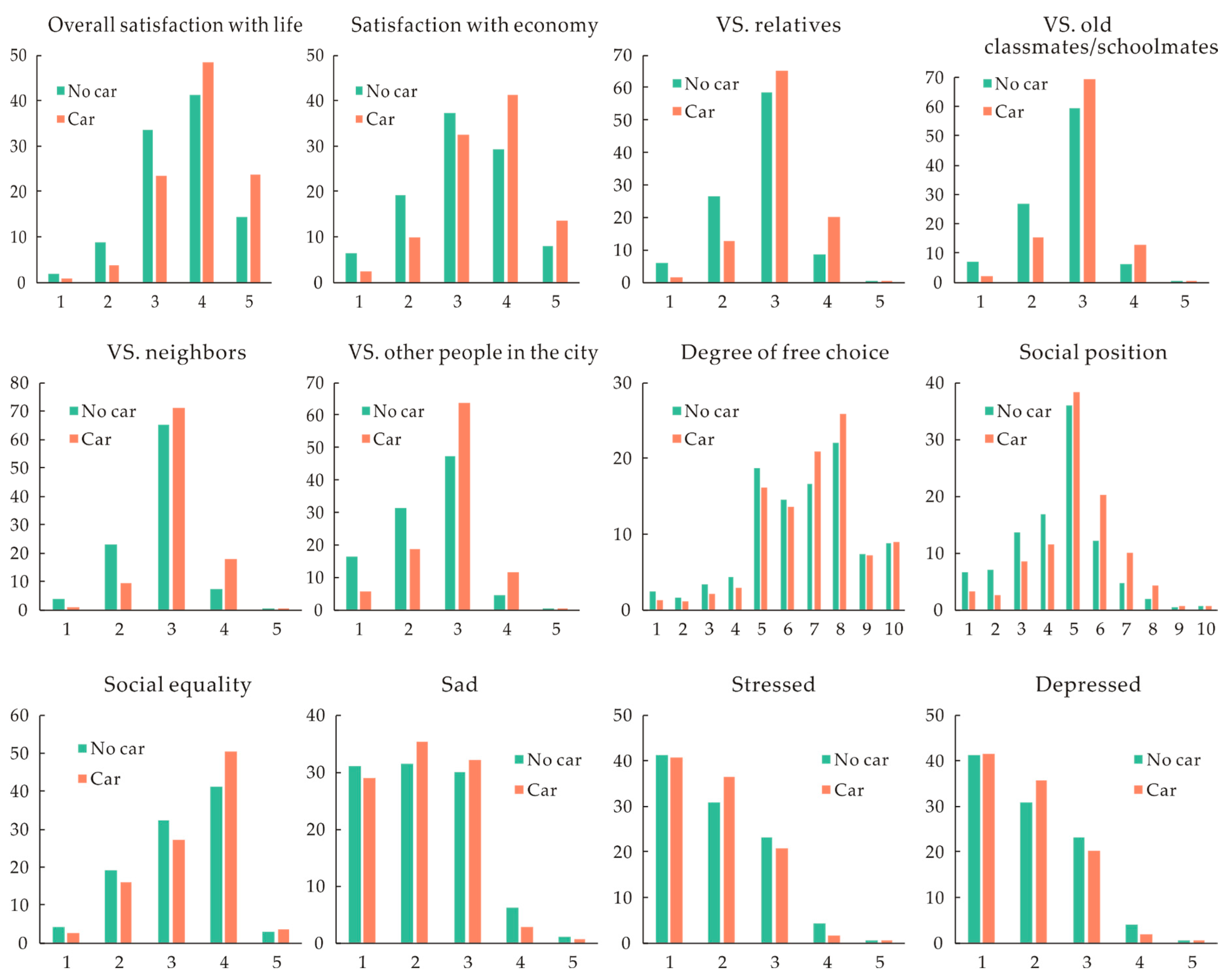
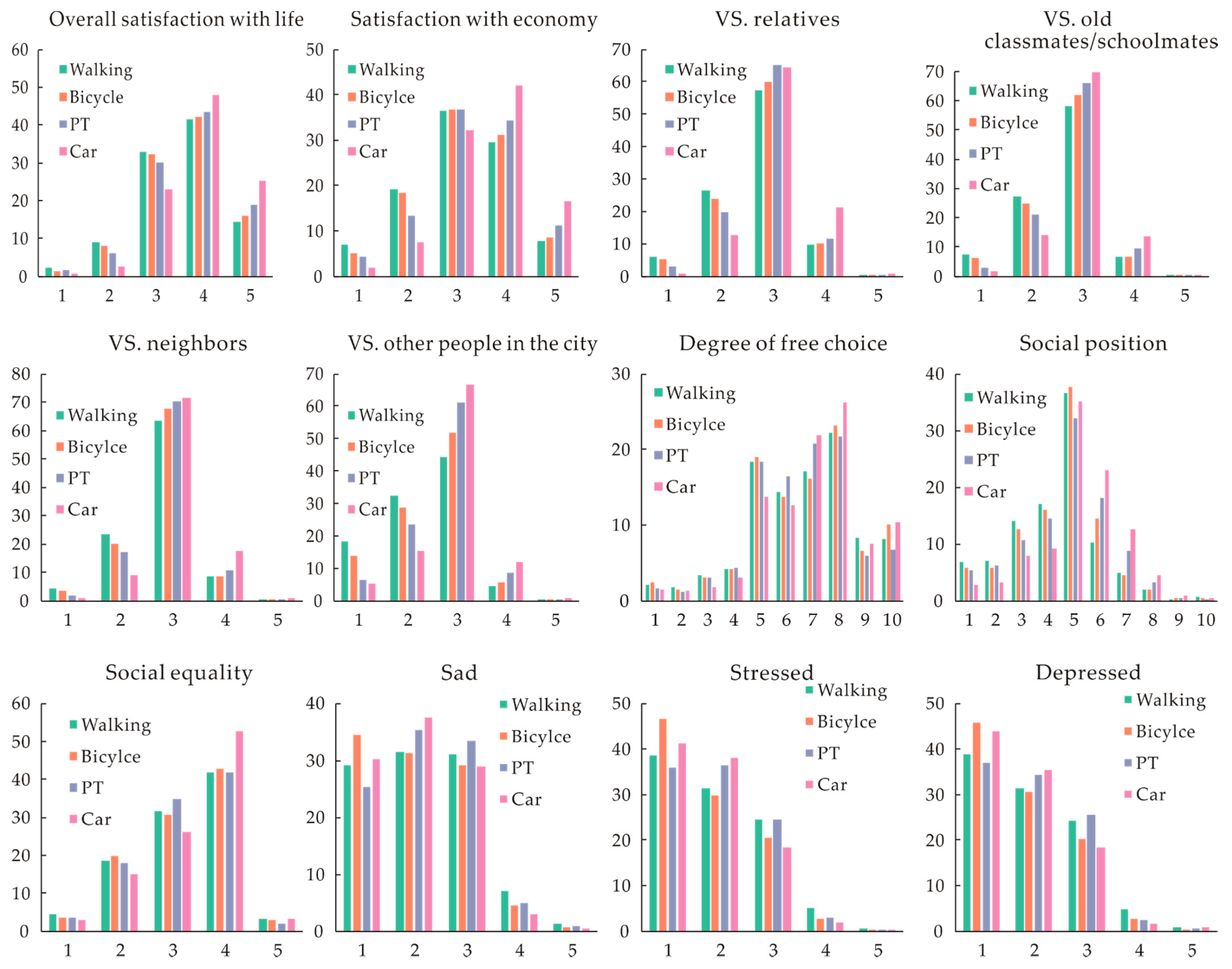
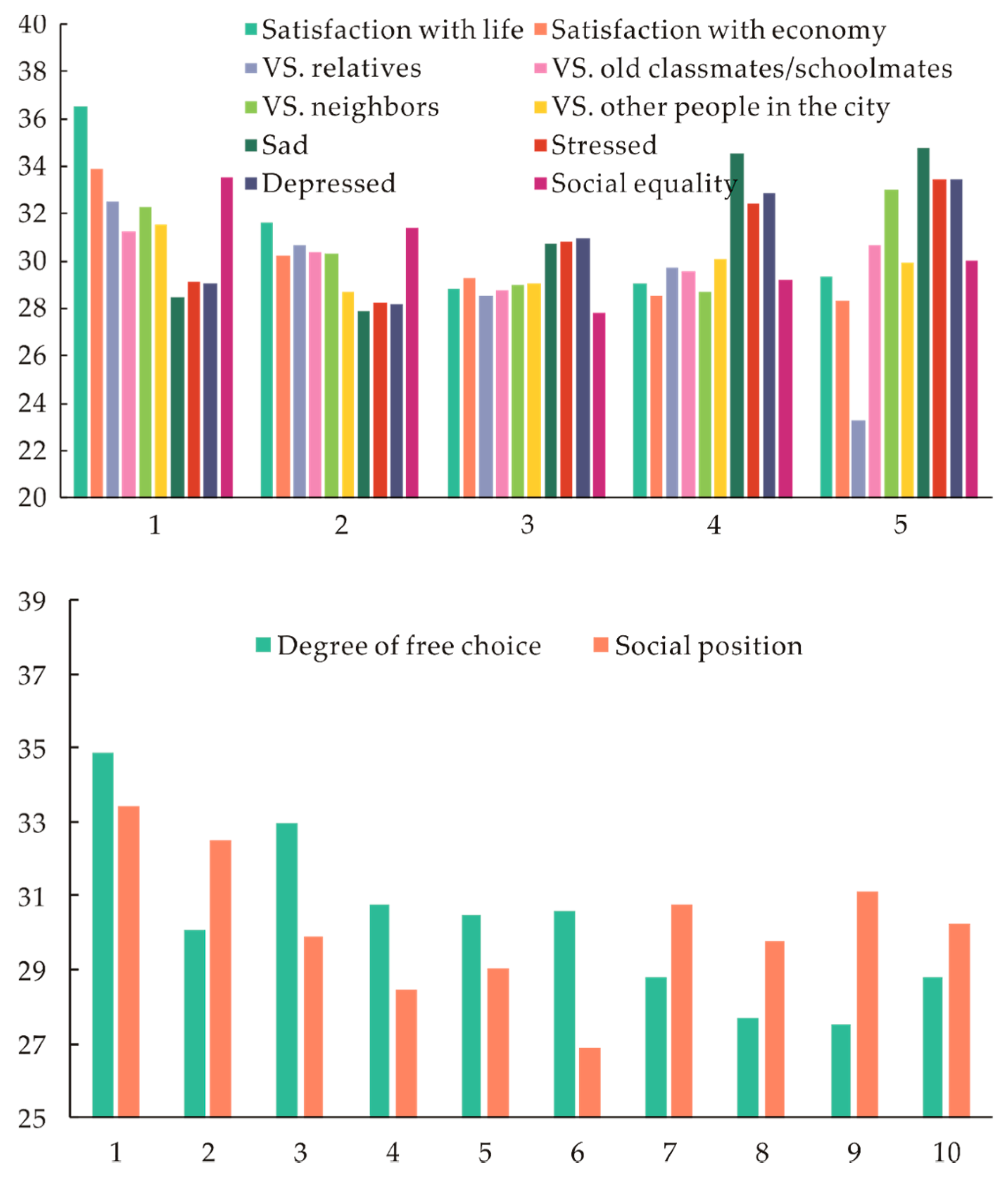
4.1. Descriptive Analysis

Before estimating the ordered probit regression models, we first conducted a descriptive analysis to investigate the associations between the travel-related factors and the twelve items of SWB. Figure 1 and Figure 2 present the distributions of the SWB measures considering car ownership and modal split, respectively. It can be seen that, for the items of satisfaction with life, the proportions of people who reported high satisfaction with life (>3) amongst the group whose family own car(s) are larger than those amongst the group whose family own no car. Similarly, people in the owning-car group are more likely to report high satisfaction with societal perception such as degree of free choice, social position, and social equality. It seems that people in the group without car displayed more negative emotions.

Figure 2 illustrates that the distribution trends of SWB measures for commuters traveled by walking, bicycle, PT, and car are similar. For instance, most people scored 3 or 4 for their satisfaction with life, 5 to 8 for degree of free choice and 5 for social position. Nevertheless, it appears that respondents who commuted by private car are more likely to give high grades to the self-evaluations of cognitive SWB than those commuted by other travel modes. It indicates that the cognitive SWB of people who commuted by car is highest. Figure 2 also shows that people rode to work are more likely to report lowest emotional SWB.

Figure 3 presents the average commuting time of each subjective well-being measure. On the whole, it seems that, for the items of satisfaction with life and societal perception, the longer commuting time is consistent with lower cognitive SWB. In terms of negatively emotional SWB, people with longer commuting time may report more frequency of sadness, stress, and depression. time To clarify the effects of travel-related factors on cognitive and affective SWB, the multivariate analyses using ordered regression models in the next section will provide further findings.

4.2. Multivariate Analysis

4.2.1 Satisfaction with Life

With the first 5000 iterations as burn-in iteration, sufficient iterations (10,000 times) has been simulated for the sample and model convergence was achieved.

Table 3. Ordered probit regression results on satisfaction with life. BCI: Bayesian credible interval.

	Model 1 (Overall Satisfaction with Life)		Model 2 (Satisfaction with Economy)		Model 3 (Versus Relatives)		Model 4 (Versus Old Classmates/Schoolmates)		Model 5 (Versus Neighbors)		Model 6 (Versus Other People in the City)
	Mean (S.D.)	95% BCI	Mean (S.D.)	95% BCI	Mean (S.D.)	95% BCI	Mean (S.D.)	95% BCI	Mean (S.D.)	95% BCI	Mean (S.D.)	95% BCI
Intercept	0.327 (0.214)	(−0.096, 0.755)	−0.808 * (0.210)	(−1.220, −0.392)	−0.332 (0.223)	(−0.769, 0.102)	0.0243 (0.223)	(−0.423, 0.465)	−0.476 * (0.233)	(−0.932, −0.019)	−1.135 * (0.220)	(−1.569, −0.701)
Gender (female = 1)	0.070 * (0.021)	(0.028, 0.112)	0.085 * (0.020)	(0.045, 0.126)	−0.015 (0.022)	(−0.058, 0.027)	0.047 * (0.022)	(0.004, 0.089)	0.034 (0.022)	(−0.009, 0.078)	0.007 (0.021)	(−0.035, 0.048)
Age	−0.015 * (0.006)	(−0.028, −0.002)	−0.031 * (0.006)	(−0.044, −0.017)	−0.032 * (0.007)	(−0.046, −0.018)	−0.054 * (0.007)	(−0.068, −0.039)	−0.024 * (0.007)	(−0.039, −0.010)	0.001 (0.007)	(−0.013, 0.014)
Age squared	0.0003 * (0.000)	(0.0001, 0.0005)	0.0005 * (0.00007)	(0.000, 0.0007)	0.0004 * (0.0001)	(0.000, 0.0005)	0.0006 * (0.00008)	(0.0005, 0.0008)	0.0003 * (0.0001)	(0.0002, 0.0005)	0.00004, (0.0001)	(−0.000, 0.0002)
Marriage (married =1)	0.164 * (0.034)	(0.098, 0.231)	0.015 (0.034)	(−0.052, 0.082)	0.098 * (0.036)	(0.028, 0.168)	0.121 * (0.036)	(0.049, 0.191)	0.061 (0.037)	(−0.011, 0.135)	0.051 (0.035)	(−0.020, 0.120)
Education (reference: primary school or below)
Junior secondary	−0.020 (0.026)	(−0.071, 0.032)	−0.085 * (0.025)	(−0.135, −0.034)	0.008 (0.028)	(−0.046, 0.062)	−0.063 * (0.028)	(−0.117, −0.008)	0.108 * (0.028)	(0.053, 0.163)	0.056 * (0.027)	(0.005, 0.109)
High school	0.045 (0.036)	(−0.026, 0.116)	−0.093 * (0.036)	(−0.162, −0.023)	0.035 (0.038)	(−0.038, 0.110)	−0.063 (0.039)	(−0.139, 0.013)	0.096 * (0.039)	(0.018, 0.172)	0.075 * (0.037)	(0.0002, 0.149)
College or above	0.154 * (0.042)	(0.070, 0.235)	0.073 (0.040)	(−0.006, 0.153)	0.156 * (0.043)	(0.071, 0.240)	0.082 (0.044)	(−0.005, 0.169)	0.215 * (0.045)	(0.126, 0.305)	0.284 * (0.043)	(0.200, 0.370)
Work hours	−0.002 * (0.000)	(−0.003, −0.0006)	−0.003 * (0.0006)	(−0.005, −0.002)	−0.002 * (0.0006)	(−0.003, −0.000)	−0.002 * (0.0006)	(−0.003, −0,001)	−0.002 * (0.0006)	(−0.004, −0.001)	−0.005 * (−.0006)	(−0.006, −0.003)
Work days	−0.002 (0.002)	(−0.006, 0.003)	0.003 (0.002)	(−0.001, 0.008)	0.0006 (0.002)	(−0.004, 0.005)	0.001 (0.002)	(−0.003, 0.006)	−0.001 (0.002)	(−0.006, 0.003)	0.001 (0.002)	(−0.003, 0.006)
Hukou (non-agricultural = 1)	0.016 (0.028)	(−0.038, 0.072)	0.009 (0.028)	(−0.044, 0.064)	−0.015 (0.029)	(−0.072, 0.042)	−0.011 (0.030)	(−0.070, 0.048)	−0.118 * (0.031)	(−0.180, −0.058)	0.188 * (0.029)	(0.131, 0.245)
Household size	−0.016 * (0.005)	(−0.027, −0.005)	−0.021 * (0.005)	(−0.032, −0.010)	−0.011 (0.006)	(−0.023, 0.0005)	−0.021 * (0.006)	(−0.032, −0.009)	−0.011 (0.006)	(−0.022, 0.001)	−0.036 * (0.006)	(−0.048, −0.025)
Household income	0.147 * (0.013)	(0.121, 0.174)	0.223 * (0.013)	(0.196, 0.249)	0.213 * (0.014)	(0.185, 0.241)	0.202 * (0.014)	(0.174, 0.230)	0.243 * (0.014)	(0.214, 0.272)	0.190 * (0.014)	(0.163, 0.218)
City lever (reference: tier 4 and 5)
Tier 1	−0.189 * (0.030)	(−0.248, −0.130)	−0.158 * (0.029)	(−0.216, −0.100)	−0.183 * (0.031)	(−0.248, −0.122)	−0.094 * (0.031)	(−0.155, −0.033)	−0.183 * (0.032)	(−0.245, −0.120)	−0.144 * (0.031)	(−0.205, −0.084)
Tier 2	−0.065 * (0.030)	(−0.124, −0.005)	−0.113 * (0.030)	(−0.172, −0.054)	−0.171 * (0.032)	(−0.234, −0.108)	−0.104 * (0.032)	(−0.167, −0.041)	−0.113 * (0.033)	(−0.178, −0.047)	−0.108 * (0.032)	(−0.172, −0.047)
Tier 3	−0.061 * (0.027)	(−0.114, −0.008)	0.020 (0.026)	(−0.032, 0.072)	−0.075 * (0.028)	(−0.130, −0.020)	−0.027 (0.028)	(−0.082, 0.029)	−0.060 * (0.029)	(−0.118, −0.003)	0.031 (0.028)	(−0.024, 0.088)
Time for sleep	0.039 * (0.008)	(0.023, 0.055)	0.049 * (0.008)	(0.033, 0.065)	0.045 * (0.008)	(0.028, 0.062)	0.046 * (0.008)	(0.029, 0.063)	0.026 * (0.009)	(0.009, 0.044)	0.021 * (0.008)	(0.004, 0.038)
Injuries (yes = 1)	−0.119 * (0.039)	(−0.196, −0.044)	−0.217 * (0.038)	(−0.292, −0.143)	−0.148 * (0.039)	(−0.225, −0.072)	−0.109 * (0.040)	(−0.189, −0.033)	−0.104 * (0.041)	(−0.185, −0.025)	−0.225 * (0.039)	(−0.303, −0.148)
Hospitalization (yes = 1)	0.076 (0.047)	(−0.018, 0.167)	0.035 (0.046)	(−0.056, 0.126)	0.074 (0.049)	(−0.021, 0.173)	0.079 (0.049)	(−0.018, 0.176)	0.161 * (0.051)	(0.063, 0.259)	0.117 * (0.039)	(0.021, 0.214)
Self-reported health (reference: acceptable)
Bad	−0.219 * (0.097)	(−0.406, −0.027)	−0.243 * (0.097)	(−0.435, −0.050)	−0.465 * (0.102)	(−0.667, −0.264)	−0.410 * (0.102)	(−0.610, −0.207)	−0.414 * (0.104)	(−0.618, −0.213)	−0.328 * (0.104)	(−0.532, −0.125)
Less good	−0.200 * (0.039)	(−0.277, −0.122)	−0.197 * (0.038)	(−0.274, −0.122)	−0.147 * (0.040)	(−0.226, −0.067)	−0.131 * (0.040)	(−0.212, −0.051)	−0.187 * (0.040)	(−0.266, −0.108)	−0.146 * (0.040)	(−0.224, −0.068)
Good	0.208 * (0.025)	(0.159, 0.257)	0.277 * (0.025)	(0.229, 0.326)	0.238 * (0.026)	(0.186, 0.291)	0.268 * (0.026)	(0.217, 0.320)	0.241 * (0.027)	(0.188, 0.294)	0.262 * (0.026)	(0.212, 0.314)
Very good	0.591 * (0.030)	(0.532, 0.650)	0.659 * (0.025)	(0.600, 0.716)	0.337 * (0.031)	(0.275, 0.398)	0.465 * (0.031)	(0.404, 0.526)	0.381 * (0.032)	(0.316, 0.443)	0.418 * (0.031)	(0.357, 0.480)
Household car ownership	0.225 * (0.029)	(0.166, 0.283)	0.206 * (0.029)	(0.149, 0.262)	0.343 * (0.031)	(0.283, 0.404)	0.252 * (0.031)	(0.191, 0.313)	0.349 * (0.032)	(0.287, 0.411)	0.299 * (0.031)	(0.240, 0.359)
Commuting time	−0.0006 (0.0004)	(−0.001, 0.0001)	−0.001 * (0.0004)	(−0.002, −0.001)	−0.001 * (0.0004)	(−0.002, −0.001)	−0.001 * (0.0004)	(−0.002, −0.0004)	−0.001 * (0.0004)	(−0.002, −0.0002)	−0.002 * (0.0004)	(−0.003, −0.001)
Commuting mode (reference: walking)
Bicycle	0.013 (0.023)	(−0.032, 0.059)	0.022 (0.023)	(−0.022, 0.068)	−0.035 (0.024)	(−0.082, 0.012)	−0.007 (0.024)	(−0.055, 0.040)	−0.003 (0.025)	(−0.051, 0.046)	0.076 * (0.024)	(0.029, 0.122)
PT	0.066 (0.038)	(−0.009, 0.141)	0.154 * (0.038)	(0.079, 0.229)	0.043 (0.040)	(−0.036, 0.122)	0.122 * (0.040)	(0.044, 0.201)	0.071 (0.042)	(−0.009, 0.152)	0.207 * (0.039)	(0.128, 0.284)
Private car	0.104 * (0.047)	(0.009, 0.198)	0.223 * (0.048)	(0.129, 0.318)	0.083 (0.050)	(−0.015, 0.181)	0.127 * (0.052)	(0.024, 0.228)	0.057 (0.052)	(−0.046, 0.159)	0.133 * (0.050)	(0.034, 0.230)
${\mathit{\gamma }}_{\mathbf{2}}$	0.924 * (0.027)	(0.899, 1.005)	0.899 * (0.017)	(0.887, 0.931)	1.171 * (0.027)	(1.124, 1,200)	1.108 * (0.012)	(1.091, 1.145)	1.220 * (0.027)	(1.157, 1.252)	0.992 * (0.021)	(0.957, 1.022)
${\mathit{\gamma }}_{\mathbf{3}}$	2.100 * (0.026)	(2.074, 2.180)	1.997 * (0.010)	(1.989, 2.025)	3.050 * (0.036)	(2.992, 3.101)	3.149 * (0.019)	(3.118, 3.184)	3.381 * (0.034)	(3.293, 3.410)	2.863 * (0.028)	(2.814, 2.911)
${\mathit{\gamma }}_{\mathbf{4}}$	3.371 * (0.029)	(3.354, 3.471)	3.192 * (0.028)	(3.163, 3.221)	4.640 * (0.054)	(4.578, 4.776)	4.538 * (0.057)	(4.438, 4.694)	4.872 * (0.041)	(4.752, 4.911)	4.320 * (0.061)	(4.230, 4.473)

Notes: *. Denotes significance at the 5% level.

illustrates the results of the six ordered probit regression with respect to satisfaction with life. The negativity and positivity of the estimated mean values indicate the decreasing and increasing influences on SWB.

The results shows that owning a car may significantly and positively associated with people’s satisfaction with life, no matter the satisfaction is measured directly or based on a given specific group. Model 1 shows that longer commuting time is likely to reduce people’s overall satisfaction with life, but this effect is ambiguous, as illustrated by its 95% BCI across zero. This finding is largely in line with some previous studies conducted in China in recent years [11,29]. However, models 3 to 6 show that the effects of commuting time on the satisfactions with life is significant and negative when respondents are required to compare their life level with their familiar groups such as relatives, old classmates and schoolmates, neighbors and other people in the same city. The results also show that there is no significant disparity between the effects of commuting on foot and by bicycle on satisfaction with life, except for the satisfaction with life (versus the other people in the city). Compared to commutes by walking, commutes by PT or private car have relatively positive effect on people’s satisfaction with life, since all the corresponding coefficients (estimated mean values) of PT and private car in Table 3 are positive. However, the positive effects are not significant for all measures of satisfaction with life. For instance, it is not significant for the satisfaction with life (versus relatives and versus neighbors) for private car (95% BCI (−0.015, 0.181) in model 3 and (−0.046, 0.159) in model 5).

In terms of the controlled variables, most of them have a significant effect on satisfaction with life. Age and age squared have significant effects on satisfaction with life. The coefficients of age are negative while the coefficients of age squared are positive, indicating that the relationship between age and satisfaction with life is significant in a U-shaped manner. Increasing of age would decrease the satisfaction with life first but the effect will turn from negative to positive when age reach or exceed the turning point. A probable explanation is that middle-aged people usually take on heavier household responsibility for having elderly and children in their family, considering many Chinese families are within a multi-generational household structure. The relationship between work hours and satisfaction with life is significant at the 5% level. Longer work hours reduce the levels of satisfaction with life and this negative relationship is robust (significances in all the six models). However, results show no significant relationship between work days and satisfaction with life. As the estimated mean values shown, the number of people in a family has a negative effect on satisfaction with life, and this negative effect is strong in models 1, 2, 4, and 6. It is not unexpected that household income has a strongly positive effect on satisfaction with life. Table 3 shows that all the signs of the coefficients of household income remain the same and 95% BCI do not cross zero, indicating that this positive effect is robust.

Table 3 also reports that increasing time for sleep tend to have a positive impact on satisfaction and this effect is significant and quite robust. This is in line with [24] who analyzed the relationship between satisfaction with life and time-use for domains based on the data from Germany. Moreover, we find that there is a significant correlation between health condition (both objective and subjective self-report) and satisfaction with life. Hence, it is important to control for health condition to avoid a potential bias for the results. Unfortunately, most prior researches ignored controlling for health condition. The results from Table 3 also show that there is no clear evidence that hukou status has a significant effect on satisfaction with life. Interestingly, there is significant relationship between city levels and satisfaction with life. Living in larger cities is generally associated with lower satisfaction with life.

4.2.2. Satisfaction with Specific Societal Perception

Table 4. Ordered probit regression results on specific societal perception.

	Model 7 (Degree of Free Choice)		Model 8 (Social Position)		Model 9 (Social Equality)
	Mean (S.D.)	95% BCI	Mean (S.D.)	95% BCI	Mean (S.D.)	95% BCI
Household car ownership	0.069 * (0.028)	(0.014, 0.123)	0.236 * (0.028)	(0.180, 0.291)	0.154 * (0.030)	(0.096, 0.214)
Commuting time	−0.001 * (0.0003)	(−0.002, −0.0002)	−0.001 * (0.0004)	(−0.002, −0.0007)	−0.0001 (0.0004)	(−0.0008, 0.0007)
Commuting mode (reference: walking)
Bicycle	−0.014 (0.022)	(−0.058, 0.030)	0.015 (0.022)	(−0.027, 0.058)	−0.001 (0.023)	(−0.047, 0.044)
PT	−0.019 (0.038)	(−0.092, 0.052)	0.108 * (0.036)	(0.035, 0.181)	0.060 (0.038)	(−0.017, 0.134)
Private car	0.066 (0.046)	(−0.022, 0.157)	0.162 * (0.047)	(0.068, 0.253)	0.089 (0.048)	(−0.005, 0.185)
${\mathit{\gamma }}_{\mathbf{2}}$	0.245 * (0.016)	(0.215, 0.279)	0.416 * (0.012)	(0.392, 0.442)	1.041 * (0.002)	(1.040, 1.046)
${\mathit{\gamma }}_{\mathbf{3}}$	0.547 * (0.020)	(0.512, 0.592)	0.934 * (0.015)	(0.905, 0.964)	1.925 * (0.005)	(1.921, 1.935)
${\mathit{\gamma }}_{\mathbf{4}}$	0.813 * (0.022)	(0.776, 0.866)	1.405 * (0.016)	(1.372, 1.437)	3.777 * (0.023)	(3.729, 3.790)
${\mathit{\gamma }}_{\mathbf{5}}$	1.513 * (0.024)	(1.472, 1.571)	2.449 * (0.019)	(2.415, 2.487)
${\mathit{\gamma }}_{\mathbf{6}}$	1.909 * (0.024)	(1.866, 1.969)	3.074 * (0.021)	(3.038, 3.116)
${\mathit{\gamma }}_{\mathbf{7}}$	2.364 * (0.024)	(2.321, 2.421)	3.592 * (0.022)	(3.549, 3.635)
${\mathit{\gamma }}_{\mathbf{8}}$	3.083 * (0.025)	(3.038, 3.138)	4.083 * (0.030)	(4.029, 4.143)
${\mathit{\gamma }}_{\mathbf{9}}$	3.450 * (0.025)	(3.403, 3.502)	4.292 * (0.036)	(4.233, 4.373)

Notes: *. Denotes significance at the 5% level. For the sake of the research purpose and paper length limitation, only the parameters of the travel-related variables are reported. The detailed regression result is available upon request.

presents the results of satisfaction with specific societal perception. In line with our descriptive findings, the effects of household car ownership suggest that car ownership is positively correlated with the satisfaction with specific societal perception because all the estimated mean values are positive and the corresponding 95% BCI do not cross zero. Commuting time has a negative effect on satisfaction with societal perceptions, but its effect on social equality is not significant (95% BCI = (−0.0008, 0.0007)). When it comes to commuting modes, the results show that there is no significant disparity among the effects of different travel modes on satisfaction with societal perceptions except social position. Nevertheless, people who commute by private car are more likely to report higher levels of satisfaction with societal perception than people who commute by walking, bicycle and PT, which is consistent with our aforementioned descriptive analysis.

4.2.3. Emotional SWB

The relationships between travel-related variables and three negative emotions including sad, stressed, and depressed are reported in

Table 5. Ordered probit regression results on emotional subjective well-being (SWB).

	Model 10 (Sad)		Model 11 (Stressed)		Model 12 (Depressed)
	Mean (S.D.)	95% BCI	Mean (S.D.)	95% BCI	Mean (S.D.)	95% BCI
Household car ownership	0.044 (0.030)	(−0.015, 0.102)	0.013 (0.030)	(−0.045, 0.072)	0.022 (0.030)	(−0.037, 0.080)
Commuting time	0.001 * (0.0004)	(0.0005, 0.002)	0.0005 (0.0004)	(−0.0003, 0.001)	0.0005 (0.0004)	(−0.0002, 0.001)
Commuting mode (reference: walking)
Bicycle	−0.113 * (0.023)	(−0.159, −0.068)	−0.133 * (0.024)	(−0.181, −0.085)	−0.104 * (0.024)	(−0.150, −0.056)
PT	−0.0001 (0.039)	(−0.077, 0.075)	0.069 (0.040)	(−0.008, 0.148)	0.076 (0.040)	(−0.002, 0.155)
Private car	−0.081 (0.049)	(−0.176, 0.016)	−0.024 (0.049)	(−0.121, 0.073)	−0.019 (0.050)	(−0.117, 0.080)
${\mathit{\gamma }}_{\mathbf{2}}$	0.859 * (0.010)	(0.849, 0.884)	0.856 * (0.009)	(0.839, 0.880)	0.852 * (0.009)	(0.838, 0.861)
${\mathit{\gamma }}_{\mathbf{3}}$	2.112 * (0.013)	(2.085, 2.124)	1.997 * (0.009)	(1.990, 2.031)	2.016 * (0.008)	(1.999, 2.039)
${\mathit{\gamma }}_{\mathbf{4}}$	3.020 * (0.018)	(2.999, 3.049)	2.879 * (0.033)	(2.814, 2.914)	2.833 * (0.014)	(2.816, 2.879)

Notes: ^* Denotes significance at the 5% level. For the sake of the research purpose and paper length limitation, only the parameters of the travel-related variables are reported. The detailed regression result is available upon request.

. As expected, household car ownership has a slightly positive effect on negatively emotional SWB, as inferred from the estimated mean values and 95% BCI. Longer commuting time is associated with stronger feeling of sad (mean = 0.001, 95% BCI = (0.0005, 0.002)), while the effects on stressed and depressed emotions are ambiguous. In line with our aforementioned descriptive analysis and Morris and Guerra [10], commuting by bicycle is associated with least negative emotions than commuting by other modes. Compared with walking, commuting by private car also illustrates less sad, stressed, and depressed feelings, while the corresponding 95% BCIs show the disparities are insignificant. Drawing on the data from ATUS, they stated that the relationship between mood and mode tends to be weak, and people travelling by bicycle have the most positive mood while car users have the second most positive emotions [10]. Another study based on the same dataset from USA also showed the similar conclusion [21].

4.3. Wald Test

In this section, we used the Wald test to examine whether or not adding car ownership and commuting variables into the models can significantly improve the prediction of individual SWB [49].

Table 6. Wald test results for each SWB independent variables.

Model.	Chi-Square	df.	P-value
Satisfaction with life
Overall satisfaction with life	84.23	5	0.000
Satisfaction with economy	116.92	5	0.000
Versus relatives	179.81	5	0.000
Versus old classmates/schoolmates	108.32	5	0.000
Versus neighbors	148.83	5	0.000
Versus other people in the city	157.26	5	0.000
Societal perception
Degree of free choice	24.24	5	<0.001
Social position	128.61	5	0.000
Social equality	43.53	5	0.000
Emotional SWB
Sad	39.21	5	0.000
Stressed	49.92	5	0.000
Depressed	37.21	5	0.000

presents the results of Wald test for all cognitive and affective SWB variables. It shows whether adding car ownership and commuting independent variables into the models yields significant differences. Because all chi-square values are associated with a P-value which is less than 0.01, adding car ownership, commuting time, and modes variables are considered to improve the prediction accuracy for all the twelve items of individual SWB. It indicates that travel-related factors should be included as independent variables when assessing individual SWB.

5. Conclusions and Discussion

In this paper, we provide additional insights into the linkages between household car ownership, commuting time, transportation modes and different aspects of SWB based on a national survey in China. There is a need to understand this relationship in the context of such a big emerging market, especially considering that most previous researches were carried out in developed countries, whereas results may not apply to the Chinese situation. Furthermore, this study includes both cognitive and affective aspects of individual SWB and extends the generic cognitive SWB to the relative measures of satisfaction with life and societal perceptions. A series of ordered probit models based on Bayesian inference were utilized to demonstrate how and to what extent travel-related variables affect individual SWB.

Results show that car ownership has a significant effect on cognitive SWB but quite limited influences on affective SWB. Moreover, people whose households own car(s) may report higher satisfactions with life and societal perceptions but also higher negative emotions (e.g., sad, stressed, and depressed), though the effects on emotions are weak. On the whole, increasing commuting time has a negative effect (albeit perhaps weakly sometimes) on individual SWB, both cognitive and affective aspects. This finding is quite consistent with the studies in other countries [9,38]. Relatively, this negative effect is more obvious on satisfactions with life and societal perceptions than on emotions. Compared to walking, commuting by a private car is associated with higher satisfactions with life and societal perceptions. People who commuted by car are prone to report higher cognitive SWB, while this positive trend does not suit for the affective SWB. Commuting by bicycle, however, is associated the lowest negative emotions among all the four modes. In this paper, we extended the measure of satisfactions with life to different specific perspectives. Despite the self-reported average grades of satisfactions with life compared to relatives, classmates/schoolmates, neighbors and other people in the city are far lower than the direct measurement, the analyses results illustrate that the effects of car ownership, commuting time and modes on different measured satisfactions with life do not make big differences since the directions of the estimated mean values are same. Meanwhile, the Wald test demonstrates that adding car ownership, commuting time and modes into the modeling framework contribute to improve individual SWB prediction, which indicates that these travel-related factors are necessary when assessing individual SWB.

Some significant relationships are also found between SWB and socioeconomic variables of individual/household, such as age, education, and income. Since analyzing these relationships is not the focus of this paper, we do not expand the descriptions here. However, we pay more attention to the two special variables related to the Chinese context, hukou and city-tier (perhaps applied to other countries). According to the results, there is no clear evidence that hukou has a significant effect on individual satisfaction with life. People living in big and central cities (tier 1 or 2 cities) report lower satisfaction with life than those who live in smaller cities, which indicates that people living in small cities are more satisfied with life than those living in large- and mega-cities [50].

The findings of this study have plenty of policy implications with respect to improve residents’ SWB in China. First, commuting time indeed has a negative effect on individual SWB, both cognitive and affective aspects. Long commuting time will increase people’s negative emotions and decrease their satisfaction with life. Sustainable urban and transportation development therefore need to not only decrease commuting time but also increase people’s well-being, in the sense that it is necessary to reduce the job-housing imbalance and commuting time through careful spatial planning. Additionally, reducing travel time can also benefit the sustainable development of cities and social well-being regarding carbon emission and energy consumption.

Second, the results indicate that car ownership and commuting by car are associated with high cognitive SWB. This may be attributed to the reality that China is still a developing country. Despite China has been the second-biggest economy in the world, the per capita income is far lower than that of developed countries. The motor vehicles per 1000 people in China is 83, which is far lower than European and North American countries (e.g., 797 for USA, 578 for France, 528 for the Netherlands) [51]. Many families in China, especially in small cities, cannot afford to buy and maintain a car. This means that owning a car to some degree presents household economic power. Car ownership and driving are positively associated with people’s cognitive SWB at the present stage. As urbanization process continues and becomes deeper and wider, private car use would increase as well in China. Therefore, it leads to some additional challenges to urban planners and transportation managers. They may need to pay much effort to reduce the traffic congestion since traffic jams have become a bottleneck in many Chinese cities. Moreover, prior studies from developed countries have shown that terrible traffic conditions would obviously decrease individual SWB [10,38]. Moreover, compared to the use of sustainable transport modes (i.e., public transport, bicycle), car use generates more carbon emission and energy consumption. Car-sharing and new-energy automobiles should be encouraged and supported since air pollution is significantly and negatively associated with individual SWB [52,53].

Third, our study also illustrates that there is a significantly positive correlation between cycling and affective SWB (albeit positive emotions are not examined). Unfortunately, the cycling environment in China needs much improvement, e.g., separate bicycle lanes (motorway and bicycle lanes are always mixed in many Chinese cities), dedicated bike parking slots. Meanwhile, the direct exposure under the serious air pollution also decreases the willingness of cycling to work. This will also accommodate the new bicycle-sharing schemes in China, such as Mobike and OFO, which has attracted a large number of users in recent years. Furthermore, the integrated policies oriented to the combination of bike and transit may encourage wider use of active modes, which in consequence can increase people’s SWB.

References

1. De Vos, J.; Schwanen, T.; Van Acker, V.; Witlox, F. Travel and subjective well-being: A focus on findings, methods and future research needs. Transp. Rev. 2013, 33, 421–442. [Google Scholar] [CrossRef]
2. Ura, K.; Alkire, S.; Zangmo, T. Bhutan. Gross national happiness and the GNH index. In World Happiness Report; Helliwell, J., Layard, E., Sachs, J., Eds.; The Earth Institute: New York, NY, USA, 2012; pp. 108–159. [Google Scholar]
3. Stiglitz, J.E.; Sen, A.; Fitoussi, J.-P. Report by the Commission on the Measurement of Economic Performance and Social Progress; CMEPSP: Paris, France, 2009; Available online: https://www.cps.fgv.br/ibrecps/nw/rapport_anglais_1-18.pdf (accessed on 5 February 2018).
4. Tiefenbach, T.; Kohlbacher, F. Subjective well-being across gender and age in Japan: An econometric analysis. In Gender, Lifespan and Quality of Life: An International Perspective; Eckermann, E., Ed.; Springer: New York, NY, USA, 2014; pp. 183–201. ISBN 9789400778283. [Google Scholar]
5. Cao, J.; Wang, D. The association between travel and satisfaction with travel and life: Evidence from the Twin Cities. In Mobility, Sociability and Well-Being of Urban Living; Wang, D., He, S., Eds.; Springer: Berlin, Germany, 2016; pp. 151–167. ISBN 9783662481837. [Google Scholar]
6. Abou-Zeid, M.; Ben-Akiva, M. Well-being and activity-based models. Transportation 2012, 39, 1189–1207. [Google Scholar] [CrossRef] [Green Version]
7. Wang, F.; Wang, D. Place, geographical context and subjective well-being: State of art and future directions. In Gender, Lifespan and Quality of Life: An International Perspective; Eckermann, E., Ed.; Springer: New York, NY, USA, 2014; pp. 183–201. ISBN 9789400778283. [Google Scholar]
8. Ettema, D.; Gärling, T.; Olsson, L.E.; Friman, M. Out-of-home activities, daily travel, and subjective well-being. Transp. Res. Part A Policy Pract. 2010, 44, 723–732. [Google Scholar] [CrossRef]
9. Stutzer, A.; Frey, B.S. Stress that doesn’t pay: The commuting paradox. Scand. J. Econ. 2008, 110, 339–366. [Google Scholar] [CrossRef]
10. Morris, E.A.; Guerra, E. Mood and mode: Does how we travel affect how we feel? Transportation 2015, 42, 25–43. [Google Scholar] [CrossRef]
11. Zhu, Z.; Li, Z.; Chen, H.; Liu, Y.; Zeng, J. Subjective well-being in China: How much does commuting matter? Transportation 2017. [Google Scholar] [CrossRef]
12. Diener, E.; Emmons, R.A.; Larsen, R.J.; Griffin, S. The satisfaction with life scale. J. Pers. Assess. 1985, 49, 71–75. [Google Scholar] [CrossRef]
13. Watson, D.; Clark, L.A.; Tellegen, A. Development and validation of brief measures of positive and negative affect: The PANAS scales. J. Pers. Soc. Psychol. 1988, 54, 1063–1070. [Google Scholar] [CrossRef]
14. Västfjäll, D.; Friman, M.; Gärling, T.; Kleiner, M. The measurement of core affect: A Swedish self-report measure derived from the affect circumplex. Scand. J. Psychol. 2002, 43, 19–31. [Google Scholar] [CrossRef]
15. Diener, E.; Wirtz, D.; Tov, W.; Kim-Prieto, C.; Choi, D.; Oishi, S.; Biswas-Diener, R. New well-being measures: Short scales to assess flourishing and positive and negative feelings. Soc. Indic. Res. 2010, 97, 143–156. [Google Scholar] [CrossRef]
16. Ettema, D.; Gärling, T.; Eriksson, L.; Friman, M.; Olsson, L.E.; Fujii, S. Satisfaction with travel and subjective well-being: Development and test of a measurement tool. Transp. Res. Part F Traffic Psychol. Behav. 2011, 14, 167–175. [Google Scholar] [CrossRef]
17. De Vos, J.; Schwanen, T.; Van Acker, V.; Witlox, F. How satisfying is the scale for travel satisfaction. Transp. Res. Part F Traffic Psychol. Behav. 2015, 29, 121–130. [Google Scholar] [CrossRef]
18. Luttmer, E.F. Neighbors as negatives: Relative earnings and well-being. Q. J. Econ. 2005, 120, 963–1002. [Google Scholar]
19. Martin, A.; Goryakin, Y.; Suhrcke, M. Does active commuting improve psychological wellbeing? Longitudinal evidence from eighteen waves of the British Household Panel Survey. Prev. Med. 2014, 69, 296–303. [Google Scholar] [CrossRef]
20. St-Louis, E.; Manaugh, K.; van Lierop, D.; El-Geneidy, A. The happy commuter: A comparison of commuter satisfaction across modes. Transp. Res. Part F Traffic Psychol. Behav. 2014, 26, 160–170. [Google Scholar] [CrossRef]
21. Zhu, J.; Fan, Y. Daily Travel Behavior and Emotional Well-Being: A Comprehensive Assessment of Travel-Related Emotions and the Associated Trip and Personal Factors. 2017. Available online: http://hdl.handle.net/11299/185433 (accessed on 10 February 2018).
22. Dickerson, A.; Hole, A.R.; Munford, L.A. The relationship between well-being and commuting revisited: Does the choice of methodology matter? Reg. Sci. Urban Econ. 2014, 49, 321–329. [Google Scholar] [CrossRef]
23. Gao, Y.; Rasouli, S.; Timmermans, H.; Wang, Y. Understanding the relationship between travel satisfaction and subjective well-being considering the role of personality traits: A structural equation model. Transp. Res. Part F Traffic Psychol. Behav. 2017, 49, 110–123. [Google Scholar] [CrossRef]
24. Lorenz, O. Does commuting matter to subjective well-being? J. Transp. Geogr. 2018, 66, 180–199. [Google Scholar] [CrossRef] [Green Version]
25. Bergstad, C.J.; Gamble, A.; Gärling, T.; Hagman, O.; Polk, M.; Ettema, D.; Friman, M.; Olsson, L.E. Subjective well-being related to satisfaction with daily travel. Transportation 2011, 38, 1–15. [Google Scholar] [CrossRef]
26. Gärling, T.; Gärling, A.; Loukopoulos, P. Forecasting psychological consequences of car use reduction: A challenge to an environmental psychology of transportation. Appl. Psychol. 2002, 51, 90–106. [Google Scholar] [CrossRef]
27. Abou-Zeid, M.; Fujii, S. Travel satisfaction effects of changes in public transport usage. Transportation 2016, 43, 301–314. [Google Scholar] [CrossRef]
28. Roberts, J.; Hodgson, R.; Dolan, P. “It’s driving her mad”: Gender differences in the effects of commuting on psychological health. J. Health Econ. 2011, 30, 1064–1076. [Google Scholar] [CrossRef] [PubMed]
29. Nie, P.; Sousa-Poza, A. Commute time and subjective well-being in urban China. China Econ. Rev. 2018, 48, 188–204. [Google Scholar] [CrossRef] [Green Version]
30. Rüger, H.; Pfaff, S.; Weishaar, H.; Wiernik, B.M. Does perceived stress mediate the relationship between commuting and health-related quality of life? Transp. Res. Part F Traffic Psychol. Behav. 2017, 50, 100–108. [Google Scholar] [CrossRef]
31. Jain, J.; Lyons, G. The gift of travel time. J. Transp. Geogr. 2008, 16, 81–89. [Google Scholar] [CrossRef]
32. Olsson, L.E.; Gärling, T.; Ettema, D.; Friman, M.; Fujii, S. Happiness and satisfaction with work commute. Soc. Indic. Res. 2013, 111, 255–263. [Google Scholar] [CrossRef]
33. Ory, D.T.; Mokhtarian, P.L. When is getting there half the fun? Modeling the liking for travel. Transp. Res. Part A Policy Pract. 2005, 39, 97–123. [Google Scholar] [CrossRef] [Green Version]
34. Gatersleben, B.; Uzzell, D. Affective appraisals of the daily commute: Comparing perceptions of drivers, cyclists, walkers, and users of public transport. Environ. Behav. 2007, 39, 416–431. [Google Scholar] [CrossRef]
35. Mokhtarian, P.L.; Papon, F.; Goulard, M.; Diana, M. What makes travel pleasant and/or tiring? An investigation based on the French National Travel Survey. Transportation 2015, 42, 1103–1128. [Google Scholar] [CrossRef]
36. De Vos, J.; Mokhtarian, P.L.; Schwanen, T.; Van Acker, V.; Witlox, F. Travel mode choice and travel satisfaction: Bridging the gap between decision utility and experienced utility. Transportation 2016, 43, 771–796. [Google Scholar] [CrossRef]
37. Kahneman, D.; Krueger, A.B.; Schkade, D.A.; Schwarz, N.; Stone, A.A. A survey method for characterizing daily life experience: The day reconstruction method. Science 2004, 306, 1776–1780. [Google Scholar] [CrossRef] [PubMed]
38. Choi, J.; Coughlin, J.; D’Ambrosio, L. Travel time and subjective well-being. Transp. Res. Rec. 2013, 2357, 100–108. [Google Scholar] [CrossRef]
39. Measuring National Well-being, Commuting and Personal Well-Being. Available online: http://webarchive.nationalarchives.gov.uk/20160105231823/http://www.ons.gov.uk/ons/rel/wellbeing/measuring-national-well-being/commuting-and-personal-well-being--2014/art-commuting-and-personal-well-being.html (accessed on 12 February 2018).
40. Lindström, M. Means of transportation to work and overweight and obesity: A population-based study in southern Sweden. Prev. Med. 2008, 46, 22–28. [Google Scholar] [CrossRef] [PubMed]
41. Nordbakke, S.; Schwanen, T. Well-being and mobility: A theoretical framework and literature review focusing on older people. Mobilities 2014, 9, 104–129. [Google Scholar] [CrossRef]
42. Chng, S.; White, M.; Abraham, C.; Skippon, S. Commuting and wellbeing in London: The roles of commute mode and local public transport connectivity. Prev. Med. 2016, 88, 182–188. [Google Scholar] [CrossRef] [PubMed] [Green Version]
43. Wheatley, D. Travel-to-work and subjective well-being: A study of UK dual career households. J. Transp. Geogr. 2014, 39, 187–196. [Google Scholar] [CrossRef] [Green Version]
44. Ye, R.; Titheridge, H. Satisfaction with the commute: The role of travel mode choice, built environment and attitudes. Transp. Res. Part D Transp. Environ. 2017, 52, 535–547. [Google Scholar] [CrossRef]
45. Ye, R. Impact of Individuals’ Commuting Trips on Subjective Well-Being: Evidence from Xi’an. Ph.D. Thesis, University College London, London, UK, 2017. [Google Scholar]
46. Albert, J.H.; Chib, S. Bayesian analysis of binary and polychotomous response data. J. Am. Stat. Assoc. 1993, 88, 669–679. [Google Scholar] [CrossRef]
47. Cowles, M.K. Accelerating Monte Carlo Markov chain convergence for cumulative-link generalized linear models. Stat. Comput. 1996, 6, 101–111. [Google Scholar] [CrossRef]
48. Martin, A.D.; Quinn, K.M.; Park, J.H. MCMCpack: Markov chain monte carlo in R. J. Stat. Softw. 2011, 42, 1–21. [Google Scholar] [CrossRef]
49. Tajalli, M.; Hajbabaie, A. On the relationships between commuting mode choice and public health. J. Transp. Health 2017, 4, 267–277. [Google Scholar] [CrossRef]
50. Chen, J.; Davis, D.S.; Wu, K.; Dai, H. Life satisfaction in urbanizing China: The effect of city size and pathways to urban residency. Cities 2015, 49, 88–97. [Google Scholar] [CrossRef]
51. NationMaster. Motor Vehicles per 1000 People: Countries Compared. Available online: http://www.nationmaster.com/country-info/stats/Transport/Road/Motor-vehicles-per-1000-people (accessed on 5 February 2018).
52. Welsch, H. Environment and happiness: Valuation of air pollution using life satisfaction data. Ecol. Econ. 2006, 58, 801–813. [Google Scholar] [CrossRef]
53. Smyth, R.; Mishra, V.; Qian, X. The environment and well-being in urban China. Ecol. Econ. 2008, 68, 547–555. [Google Scholar] [CrossRef]
Figure 1. Distributions of subjective well-being measures for household car ownership. X-axis: measurement scales, Y-axis: percent (%).
Sustainability 11 00084 g001
Figure 2. Distributions of subjective well-being measures for modal split. X-axis: measurement scales, Y-axis: percent (%).
Sustainability 11 00084 g002
Figure 3. Average commuting time of subjective well-being measures. X-axis: measurement scales, Y-average time (minutes).
Sustainability 11 00084 g003