How does the Built Environment Influence Public Transit Choice in Urban Villages in China?


1
School of Architecture, Harbin Institute of Technology (Shenzhen), Shenzhen 518000, China
2
Department of Building and Real Estate and Research Institute of Sustainable Development, The Hong Kong Polytechnic University, Hong Kong 99077, China
*
Authors to whom correspondence should be addressed.
Sustainability 2019, 11(1), 148; https://doi.org/10.3390/su11010148
Submission received: 2 November 2018
/
Revised: 13 December 2018
/
Accepted: 24 December 2018
/
Published: 28 December 2018
Abstract
:With growing traffic congestion and environmental issues, the interactions between travel behaviour and the built environment have drawn attention from researchers and policymakers to take effective measures to encourage more sustainable travel modes and to curb car trips, especially in urbanising areas where travel demand is very complicated. This paper presents how built environmental factors affect public transit choice behaviour in urban villages in China, where a large population of low-income workers are accommodated. This location had a high demand for public transit and special built environmental characteristics. Multinomial logistic regression was employed to examine both the determinants and magnitude of their influence. The results indicate that the impacts of built environments apply particularly in urban villages compared to those in formal residences. In particular, mixed land use generates an adverse effect on public transit choice, a surprising outcome which is contrary to previous common conclusions. This study contributes by addressing a special type of neighbourhood in order to narrow down the research gap in this domain. The findings help to suggest effective measures to satisfy public transit demand efficiently and also provide a new perspective for urban regeneration.
1. Introduction
For decades, public transit (PT) has gained increasing attention due to its significance in addressing environmental problems, limited urban land resources, job-housing unbalance issues as well as the demand for equity and equality of various classes of population in society with the advancing urbanisation process [1,2]. Generally, PT is regarded as a sustainable travel mode, beneficial to both individuals and the society. To individuals, it is an effective motorised mode, meeting the needs of medium and long distance urban trips, with a low level of cost and acceptable time consumption. To the society at large, PT acts as an alternative to private cars that alleviates urban congestion and air pollution, especially in dense urban areas [3,4,5].
Considering PT’s positive and significant functions, governments have implemented supportive measures and invested substantial funds to construct PT infrastructure and enhance PT services to attract more PT travel demand, while the sharing of PT has not undergone a breakthrough. For instance, in China, the fixed investment into PT grew from 66 billion yuan in 2004 to 368 billion yuan in 2014, accounting for the total investment in road transport going up from 8.96% in 2004 to 19.45% in 2014, but the share of PT passenger volume did not increase significantly, only growing from 16.3% in 2004 to 18.2% in 2014. Only a few studies have investigated the reasons for this situation, claiming that the PT travel demand was not paid as much attention as the supply of PT infrastructure [1,6]. To be specific, transport planners attached more importance to adding bus lines or bus stops, but ignored the features of the travel demand, such as what types of groups would prefer PT travel and how to satisfy their PT travel demand, or neglected to encourage more people to choose PT for daily trips. In fact, various groups of the population or different urban forms would generate distinct patterns of travel behaviour, so it would be more effective and significant to probe into a particular demand segment rather than the overall demand. Therefore, the study reported in this paper chose a segment with large demand for PT but a lack of attention to certain characteristics of population and urban form, so as to provide specific policy suggestions for PT encouragement.
In China, an urban village area is such a segment that importance needs to be attached to regarding PT travel. Urban villages are unique informal residences accommodating large amounts of migrant workers in mega-cities, especially in China. They are derived from rapid urbanisation when villagers still kept their dwelling spaces while their cultivating lands in original villages were requisitioned and surrounded by built-up areas in the city, either in urban centres or peri-urban areas in the process of urban regeneration [7]. This phenomenon is especially popular in high-speed developing metropolises in China, such as Beijing, Shanghai, Guangzhou and Shenzhen, where great job opportunities attract much external labour. In this context, for profit, the indigenous villagers or aborigines reconstructed their original cottages into multilayer buildings (under poor quality and arbitrarily without authorisation from governments) and then leased their village apartments to migrant workers at a relatively low rent compared to formal residences. A Formal Residence is defined as a type of residence approved by the government within the scope of legal urban planning and which conforms to the procedures and rules stipulated by the government. It serves as a comparison to the urban village which is a typical Informal Residence. Spontaneously, urban village areas assembled a large number of low-income workers and generated a large volume of PT commuting demand. Therefore, to meet the PT demand or in other words, to avoid the probability of car use increasing due to unsatisfied PT demand, this trend has been prompting states and localities to turn to land planning and urban design to encourage car users to switch to PT [8]. Urban villages are results of urbanisation and China is still undergoing an unprecedented surge of urbanisation and motorisation, with a rapidly expanding urban population and the rapid increase of private car ownership. Chinese cities are mimicking the suburbanisation trends and patterns of the US during the Post-World-War-Two period, which is the world’s most car-dependent nation [9]. In order to prevent an auto-dependent tendency, China’s urbanisation should follow the transit-oriented development, with the integration of land use and transport to attract more citizens to take public transit as their main trip mode choice. Besides, regeneration in urban villages is a demand for efficient land use. Therefore, it is vital to understand the relationship of the built environment with public transit behaviour in urban villages in China.
So far, there have been several, but not abundant, studies concerning PT choice. In general, previous studies have emphasised the relationship between PT and land use policies [5,10], giving rise to the trend of connecting the built environment and travel behaviour as a feasible way to switch mode choice behaviour. However, regarding to PT choice, previous studies have mainly focused on the general elements of the built environment without distinguishing its features under particular contexts of urban forms, especially in compact cities in developing countries [11]. In the last four decades, Chinese cities have undergone rapid spatial transformation and expansion, and the regeneration process is still underway. New developments in Chinese cities, however, are generally being built according to the typical modernisation following the developed world (western) style, regardless of the compact city and population features in China [12]. Particularly, the suitable built environment to meet PT demand is neglected because of the differences of transport structures between western countries and China. Subsequently, traffic problems have appeared in all directions due to the unsuitable built environments. But urban villages faced with undergoing or future renewal still have chances for better planned development if we find a more self-adapted method for urban regeneration in the aspect of built environments for sustainable transport. Also, the urban villages may face their future choice from the perspective of their transport role. Thus, urban villages play a significant role for PT development, and so PT choice behaviour in urban villages matters to sustainable urban transport.
Therefore, we pose the following research questions for this paper: How can we describe the travel behaviour of residents in urban villages in China? How influential is the built environment on travel choice behaviour? Specifically, we attempt to investigate how the unique urban form settings in China, interacting with other attributes, affect the public transit choices of residents living in urban villages in Shenzhen, China, compared to those in formal residences. Quantitative and qualitative data about travel information of residents in Shenzhen are used. We answer the research questions in the following five sections. Section 2 starts with a review of relevant literature on the status and determinants of travel mode choice behaviour. Section 3 presents an overview of the methodology, followed by results of regression models in Section 4. The final Section 5 discusses the conclusions and policy implications of our analyses.
2. Review of Factors Influencing Choice of Mode of Travel and Behaviour by Urban Travellers
Although there is a paucity of studies that have targeted the PT choice behaviour in urban villages, most have started from a more general research area focusing on the influencing factors of travel mode choice behaviour. Generally, determinants of travel mode choice behaviour are grouped into two general categories: socio-demographic factors involving demographic and socioeconomic attributes, and built environmental characteristics associated with travel mode choice.
Demographic and socioeconomic variables play critical roles in the mode-choice decision process made by travellers. A different segment of the population of different age, gender, education, income, and employment make a different travel mode choice [13,14]. Besides, household socioeconomic characteristics, such as car ownership, household size and structure, as well as household income, also significantly influence traveller mode choice [15,16]. For example, men are more likely to travel by car in commuting activities, while when it comes to shopping activities, women are more prominent car travellers [17]. Regarding employment, compared to the unemployed, the employed make a large proportion of car trips in spite of making fewer total trips [18]. Also, low-income groups have been claimed to have low mobility, but are more likely to use PT or a non-motorised mode [19].
In terms of built environmental factors, it is considered to increasingly affect travel mode choice in recent years, but the debate on its impacts is far from reaching a consensus [14]. The built environment has been summarised as 5Ds, i.e., density, diversity, design, distance to transit and destination accessibility [8]. In general, three factors: high residential density, compact cities with mixed land use, and good accessibility to public transit are considered to motivate more non-motorised, and PT travel, though this conclusion is based on research studies in the context of developed western countries [8,18]. To be specific, built environment density is linked to employment, household and building density. Higher density has been claimed to reduce car use and this encourages more people to choose PT [20]. Diversity refers to the mixed use of land. The closer the housing, job and social amenities, the less often the choice of the motorised travel mode is made [2]. Design is an important feature of urban road networks. When there is an advantageous design for walking in a community, the possibility of people choosing private cars for travel will decrease [21]. As to distance to transit and destination accessibility, a long distance to a destination or inconvenience walking to bus stops or metro stations always leads to greater car use [22,23].
PT travel demand and choice behaviour of the targeted population should be considered more carefully and in detail. There is heterogeneity among different groups of people when choosing PT services, so the measures and policies relating to PT supply could be more effective when it meets the differentiation of travel demand [24]. Among the various groups of population, PT travel behaviour of low-income populations deserves more in-depth research because they occupy a prominent position under the social background of travel equity and equality [6,25,26,27]. In particular, habitation communities with a low-income population such as urban villages are worthy of more attention because these places tend to form more massively regular PT travel demand. Therefore, the mechanism of travel behaviour is of vital importance to solving the traffic congestion of urban regions. Research studies that have been focusing on slightly different urban areas to villages but in with similar low-income populations have been conducted for years. Recently, Mushi supplemented the empirical evidence on the relationship between the built environment and mode choice in the context of the Indian city of Rajkot [28]. The study claimed that there was a strong tendency to walk or use a bicycle or auto rickshaw when locations had higher mixed land use, so the study inferred that land use policy should focus on the mix of diverse land use, which had to be location-based to support non-motorised and public transport travel [28]. In China, when Luo studied the relationship between urban fringe development and transportation supply, he compared the demand for travel by private cars and bus and the result showed that the growth of urban traffic had considerably changed the configuration of the edge of the city, but the lack of bus services made commuters dislike living in the fringe community, which led to the formation of a crowded city centre [29]. Wang investigated the impacts of built environments on travel behaviour in Hong Kong, comparing the differences between public housing and private housing and he found that people living in public and private housing in Hong Kong had significantly different built and social environments, and built environments exerted a significant influence on travel behaviour, concluding a result that density and accessibility affected private housing residents’ auto ownership, travel time and trip frequency, but had few influences on public housing dwellers [18,30].
To conclude this review, it is clear that several areas of investigation would be of interest. Apart from different groups of people, the research team also intends to investigate how travel behaviour varies in different types of neighbourhoods. Few research studies have shed light on causality between what type of residential neighbourhood one chooses and what travel behaviour one produces [17,31,32,33]. Actually, the principle of neighbourhood type choice is residential self-selection which could confound the relationships between the built environment and travel behaviour. The influence of the built environment on travel behaviour of residents may be overestimated because of residential self-selection effects [34]. To exclude the effect of residential self-selection, the most effective method is to conduct a natural experiment. If a change in built environments in a neighbourhood is observed and travel behaviour before and after this change is investigated, then we can attribute the change in travel behaviour to built environments and determine that any change in travel behaviour is irrelevant with residential self-selection.
3. Materials and Methods
3.1. Data Source and Study Area
As mentioned before, urban villages are widespread in rapidly developing cities in China. As one of the most prosperous cities, and also as a Special Economic Zone in China, Shenzhen is a typical dual-structured city with informal urban villages and formal residences co-existing for more than thirty years. Shenzhen has experienced a significant growth in population from 0.31 million since its establishment in 1979 to 12 million in 2016, about 7 million of whom live in urban villages predominately because of the low rent. This generates large demand for PT travel either for commuting or for non-commuting activities [35]. Figure 1 demonstrates the extensive distribution of urban villages in Shenzhen covering almost 60% of the built-up areas of the whole city. Taking account of these characteristics, we selected Shenzhen as our case study area.
In this study, the raw data came from a large-scale household travel survey in Shenzhen, conducted by a public sector body named the Shenzhen Urban Planning and Land Resource Research Centre (UPLR) in 2014. The survey mainly investigated four areas in the city centre and fringes where urban villages are compactly located, namely Shangxiasha (SXS), the Longhua centre (LHC), the HW tech centre (HWT) and the Tianbei community (TBC), including 8309 respondents in total. As part of the agreement with UPLR, we were eligible to select one of the four areas for our research use because the survey contained some information that was not public. We picked SXS as our study area because it is located in the city centre called the Futian district and is one of the largest urban village localities in Shenzhen (see Figure 2). More than 100 thousand people live in the SXS area, covering an area of 1.41 square kilometres and substantially 70% of the residents live in urban villages. Formal residences are also considered as a contrast.
The selected SXS area covers six urban villages and five formal residences (residential communities) (see Figure 3). As shown in Figure 3, urban villages seem to be more compact than formal residences, but in fact, the residential density is just the opposite, because the plot ratio of urban villages is much lower than that of formal residences. The survey in this area contains 249 households with 565 trips in urban villages and 263 households with 985 trips in formal residences. Also, according to our survey, there are 46 bus stops and one metro station within 500 metres of the area.
The integrated dataset in this research included not only the 2014 Shenzhen Household Travel Survey, which recorded individual, household, and travel information, but also the 2014 Shenzhen Land Use data and 2014 Shenzhen Construction Census as well, from which the built environment information could be extracted. This information was integrated as shown in Figure 4.
3.2. Travel Choice Behaviour Characteristics
Figure 5 and Figure 6 show the travel characteristics of residents in urban villages in SXS area in terms of travel mode choice and travel purpose. To provide the contrast, travel behaviour in formal residences is also shown in the two figures. As indicated in Figure 5, PT is the most popular mode for both urban villages and formal residences, while people in urban villages are more likely to travel by PT than those in their formal counterpart. Regarding travel purpose, we can see from Figure 6 that when travelling by PT, substantially 82% of people in formal residences travel for commuting, while only about 50% of residents in urban villages travel for commuting. In other words, people in urban villages travel by PT for more varied purposes, whereas those in formal residences travel by PT mainly for commuting purposes.
In addition, other travel characteristics of urban villagers also indicate significant differences compared to those of formal residents as shown in Table 1.
As can be seen from Table 1, PT features of urban villages exceed those of formal residences in every aspect, that is travel distance and travel rate apart from mode choice. Beyond that, features of travelling by non-motorised mode and by car also show significant differences. As a result, non-motorised and car mode will be considered as reference dependents in the following regression model.
3.3. Model and Variables Specification
Random utility theory is the basic core to model choice behaviour and its determinants. Given j is one option from a set of M options (j = 1, 2, …, M), the utility derived from the jth option selected by the ith individual can be expressed as . Supposing this utility is a linear function of H factors (determinants). Of these H factors, assume that R of these factors are personal related but are irrelevant to option attributes, and S of these factors are option related but are irrelevant to individuals. Assume that represents the characteristics of ith individual with R attributes (r = 1, 2, …, R), and represents the value of jth attributes (s = 1, 2, …, S), so the utility functions can be written as the following Equations (1) and (2):
is the coefficient between the the jth option and the rth characteristic, and is the coefficient between the ith individual and the sth attribute. In addition, the relationship between the utility function and its determinant variables is not quite precise, with possibilities that some factors may be excluded or the measurement of some factors is inaccurate, so an error term is added to the equation to capture this uncertainty. Therefore, the utility function is called a stochastic utility model. Only if the mth option provides the highest utility of all available options, will a person choose j = m. In other words, if is a random variable, its value j () represents the choice made by the ith individual, the probability that the ith individual chooses the mth option is shown as the following Equation (3):
To investigate the relationships between one dependent variable and independent variables, mainly when modelling the associations between a categorical (more than two categories) dependent and one or more predictor variables, a multinomial logistic regression model is widely employed in this domain [36]. Multinomial logistic regression has been performed fitting results from the evidence of previous studies [37,38]. In our study, the observed numbers of mode choices made by individuals are classified into five categories as demonstrated in Table 1. Therefore, we will use multinomial logistic regression (MNL) to examine the impacts of several variables including built environments on PT choice behaviour.
In an MNL model, all = 0, and the individual specific model is represented as Equation (4).
However, there are m equations in the MNL model but only m-1 independent unknowns. In order to standardise this problem, we set and , so the probabilities are shown in Equations (5) and (6).
A comprehensive set of variables collected and defined from four dimensions are incorporated in the model, comprising socio-demographic attributes, PT service attributes, daily travel features, and, most importantly, the built environment attributes. As mentioned in the literature review section, PT service attributes are particularly concerned in the PT choice study here. Table 2 and Table 3 display detailed statistical information of the variables. The final sample contains 565 respondents from urban villages and 985 respondents from formal residences as a contrast. The built environment variables were measured in the scale of each residence area, which is smaller and more precise than those in previous studies that were measured in TAZ scale [18,27,39]. Importantly, before applying data into the model, some diagnostic checks have been conducted to check the models. Firstly, the collinearity statistics show that the tolerance values are all larger than 0.1 and the VIF value is smaller than 10 (actually between 1 to 6) for both urban villages model and formal residences model, suggesting that there is no collinearity in the data-set of the models. Secondly, when examining the goodness-of-fit, the significance values are all larger than 0.05, proving that the model meets the assumption. Finally, the Pseudo R-Square value for the urban villages model and formal residences model are 0.634 and 0.659 respectively, which means that the model can explain most of the actual data.
4. Results
As shown in Figure 1 above, there are five types of travel modes, including non-motorised, PT, car, taxi and others. When running the MNL model with one baseline, the relative advantage of the other four modes are shown. However, to make the results easy to read and understand, travelling by non-motorised mode and car mode will act as reference dependents (a baseline) in the MNL model and we only tabulate the PT result. We omit “taxi” and “others”, because non-motorised, PT and car travelling are the main travel modes in urban villages and formal residences, and we only want to know how advantageous PT is with respect to non-motorised and car modes. The data analysis procedure using the MNL model was run for four times referring to the non-motorised mode in urban villages and formal residences respectively, and then referring to the car mode in urban villages and formal residences respectively.
Table 4 demonstrates the regression results of the PT choice regression referring to non-motorised mode, with a comparison between urban villages and formal residences. Among the built environment variables, after controlling for variables of other dimensions, only residential density shows a significant influence for both urban villages and formal residences, respectively at the 90% and 95% confidence level. Also, the direction of the influence is consistent for both urban villages and formal residences. Although urban villages and formal residences are in urban centre areas, the correlation in urban villages is less significant than that in formal residences. This implies that people in urban villages are less encouraged by density to switch from PT mode to a non-motorised mode for travel. Meanwhile, other built environmental variables did not show significant effects on travel mode. Therefore, it is not much helpful to alter built environments to attract PT travellers to shift to non-motorised travelling in urban villages.
Apart from the built environment, other variables also show significant influences. First, it is consistent with most previous studies that income remarkably affects travel mode choice behaviour [13,19]. People in different income levels exert different modes of preference. Compared to non-motorised mode, people in urban villages with incomes below CNY80 thousand are less like to choose PT, while people in formal residences with incomes above CNY200 thousand are more likely to choose PT. Secondly, travel distance is another significant factor encouraging people to choose PT instead of a non-motorised mode, but urban villages (an 16.1% increase) are less likely to be affected than formal residences (an 33.9% increase) regarding this. In addition, more factors, like age, car ownership and travel time encourage people to choose PT or non-motorised mode in formal residences, but these variables do not show a significant influence in urban villages. This could reflect that people in urban villages exhibit a more stable status than those in formal residences when they have to decide whether to choose PT or a non-motorised mode.
Table 5 illustrates the regression results of PT choice regression referring to the private car mode, with a comparison between urban villages and formal residences. Regarding the built environment variables, it is found that most of the factors show a significant influence, which is a great disparity from the results in Table 4 where only residential density matters. This suggests that the built environment plays a more important role in switching people between PT and cars than the shift between PT and non-motorised mode. Firstly, with the increase of bus stops within 500 metres, there will be a larger population with a 77.6% and 32.2% rise in urban villages and formal residences respectively to choose PT rather than car at 95% and 99% significance confidence levels. This shows that adding bus stops could encourage more PT choice and hinder car use effectively. Secondly, when residential density increases, people in urban villages will transfer from car use to PT choice, which is also consistent with most previous studies [20]. Thirdly, people in urban villages are more tolerant than those in formal residences regarding greater distances to transit. Even it takes 10 to 20 min to reach bus stops or metro stations, people in urban villages prefer to travel by PT than by car. Specifically, mixed land use shows the distinctive influence on PT choice versus car use. In the case of people in formal residences, the land use mix shows a positive effect on their PT choice, which is in accord with claims from most past research studies [2,8,20]. However, the mixed land use influences urban villages in an opposite way. To clarify, while increased land use mix is in correlation with less traveling by PT mode, in fact, people almost completely give up PT mode in urban villages. This may be due to the fact that the higher mixed land use in urban villages means a great improvement of their living environment and this would lead to higher rents in this region, which could make low-income residents have to leave this community, while those with a relatively higher income still living in this community would exert an increased proportion of car use.
In terms of other variables, more females in urban villages tend to prefer to drive instead of taking the bus than males, while there is an opposite result in the case of formal residences. Also, resident occupation demonstrates a significant influence in urban villages but not in formal residences. Regarding income, people earning 80–150 thousand yuan per year prefer PT over using cars. Although car ownership shows no significant influence in urban villages, people having no car in formal residences would be more likely to choose PT. Concerning daily travel features, a longer distance is correlated with a higher probability of choosing car mode, even though it is not in direct proportion to travel time. The reason for this could be that the congestion context could not be neglected and maybe BRT (Bus Rapid Transit) plays an important role in reducing travel time by PT.
5. Discussion and Conclusions
Urban villages highlight a spatial advantage of gathering a large population of Public Transport (PT) demand for research significance and convenience. This research has focused on a better understanding of the associations between the built environment and PT choice behaviour in urban villages, particularly in China. To discover the particularity and generality of the connection, the study has generally experienced three steps. First, a framework of influential factors was set up on the basis of previous related research and the need for this research. To be specific, four dimensions of variables were developed in the model, and they were socio-demographic, PT service, daily travel features, and most importantly the built environment attributes. Second, formal residences were incorporated as a contrast to highlight the special nature of urban villages. Third, travelling by non-motorised transport or by car were set as reference dependents when implementing multinomial logistic regression models to clearly explain the findings.
Generally, the regression results showed that built environment factors had significant influences on PT choice behaviour in urban villages, and notably played an eco-friendly and land use effective role to encourage PT choice and consequently to reduce car use. Increasing bus stops and residential density displayed a positive effect on PT choice, which was a consensus with most previous studies in the context of developed countries [14,15], while people from urban villages showed a much higher probability of choosing PT than those from formal residences. That is, for policy implications, adding bus stops around urban villages would bring a more evident effect on PT incentives and would relieve regional traffic congestion correspondingly. Interestingly, in terms of mixed land use, it did not show a positive impact on PT choice in the case of urban villages, as most previous studies have claimed [2,8,20], although the influence was still significant. Rapid urbanisation has led cities in more compact and mixed-use directions, so the inconsistency of urban villages with the developing trend could urge the regeneration of urban villages to some extent. Therefore, the findings relating people’s choice of PT with the built environment in urban villages not only provide references for traffic policymakers but also offer well-founded guidelines for urban planners.
It should be noted that there are still limitations in this paper. The sample size may not be large enough, because we only studied urban-centre villages, but we have not considered the different features of urban-fringe villages. Urban villages are confronted with transformation everywhere in the city. Our findings indicate that different location characteristics of urban villages could lead to different results of the correlation of built environment and travel behaviour.
Further studies are needed to investigate the different types of urban-centre villages and urban-fringe villages to provide type-based transformation strategies for urban villages. In addition, the model used in this paper appeared to be indirect because a reference category is necessary to explain both dependent and independent variables in the model. The model could not reflect the direct influence of the determinants but could only indicate a comparative advantage. Therefore, optimising the method and enriching the sample deserve more efforts in the future. Last, but nevertheless important, the underlying effect of residential self-selection has not yet been estimated. We have mentioned that the most effective way to exclude residential self-selection is by natural experiment. However, apply this method requires the household travel survey to be conducted twice, in order to obtain longitudinal data. This method is very hard to realise, but future studies should try to determine a suitable approach.
Author Contributions
Conceptualisation, B.X.; Data curation, L.Y.; Formal analysis, L.Y.; Funding acquisition, B.X.; Investigation, L.Y.; Methodology, L.Y.; Project administration, E.H.W.C.; Software, L.Y.; Supervision, E.H.W.C.; Writing—original draft, L.Y. and E.H.W.C.
Funding
This research was funded by the National Natural Science Foundation of China, grant number 71473060.
Acknowledgments
The authors would like to thank the anonymous reviewers for their valuable comments.
Conflicts of Interest
The authors declare no conflict of interest.
References
- Abenoza, R.F.; Cats, O.; Susilo, Y.O. Travel satisfaction with public transport: Determinants, user classes, regional disparities and their evolution. Transp. Res. A 2017, 95, 64–84. [Google Scholar] [CrossRef]
- Zailani, S.; Iranmanesh, M.; Masron, T.A.; Chan, T.-H. Is the intention to use public transport for different travel purposes determined by different factors? Transp. Res. D 2016, 49, 18–24. [Google Scholar] [CrossRef]
- Zhu, Y.; Wang, Y.; Ding, C. Investigating the influential factors in the metro choice behavior: Evidences from Beijing, China. KSCE J. Civ. Eng. 2016, 20, 2947–2954. [Google Scholar] [CrossRef]
- Haywood, L.; Koning, M.; Monchambert, G. Crowding in public transport: Who cares and why? Transp. Res. A 2017, 100, 215–227. [Google Scholar] [CrossRef] [Green Version]
- Chen, C.; Varley, D.; Chen, J. What Affects Transit Ridership? A Dynamic Analysis involving Multiple Factors, Lags and Asymmetric Behaviour. Urban Stud. 2010, 48, 1893–1908. [Google Scholar] [CrossRef]
- Serulle, N.U.; Cirillo, C. Transportation needs of low income population: A policy analysis for the Washington D.C. metropolitan region. J. Public Transp. 2016, 8, 103–123. [Google Scholar] [CrossRef]
- Zhang, L.; Ye, Y.; Chen, J. Urbanization, informality and housing inequality in indigenous villages: A case study of Guangzhou. Land Use Pol. 2016, 58, 32–42. [Google Scholar] [CrossRef]
- Ewing, R.; Cervero, R. Travel and the Built Environment. J. Am. Plann. Assoc. 2010, 76, 265–294. [Google Scholar] [CrossRef]
- Cervero, R. Transit-Oriented Development’s Ridership Bonus: A Product of Self-Selection and Public Policies. Environ. Plan. A 2007, 39, 2068–2085. [Google Scholar] [CrossRef]
- Soria-Lara, J.A.; Aguilera-Benavente, F.; Arranz-López, A. Integrating land use and transport practice through spatial metrics. Transp. Res. A 2016, 91, 330–345. [Google Scholar] [CrossRef]
- Feng, J.; Dijst, M.; Wissink, B.; Prillwitz, J. The impacts of household structure on the travel behaviour of seniors and young parents in China. J. Transp. Geogr. 2013, 30, 117–126. [Google Scholar] [CrossRef]
- Feng, J. The influence of built environment on travel behavior of the elderly in urban China. Transp. Res. D 2017, 52, 619–633. [Google Scholar] [CrossRef]
- Khan, S.; Maoh, H.; Lee, C.; Anderson, W. Toward sustainable urban mobility: Investigating nonwork travel behavior in a sprawled Canadian city. Int. J. Sustain. Transp. 2014, 10, 321–331. [Google Scholar] [CrossRef]
- Ding, C.; Wang, D.; Liu, C.; Zhang, Y.; Yang, J. Exploring the influence of built environment on travel mode choice considering the mediating effects of car ownership and travel distance. Transp. Res. A 2017, 100, 65–80. [Google Scholar] [CrossRef]
- Su, F.; Schmöcker, J.-D.; Bell, M.G.H. Mode Choice of Older People Before and After Shopping: A Study with London Data. J. Transp. Land Use 2009, 2, 29–46. [Google Scholar] [CrossRef]
- Sun, B.; Ermagun, A.; Dan, B. Built environmental impacts on commuting mode choice and distance: Evidence from Shanghai. Transp. Res. D 2017, 52, 441–453. [Google Scholar] [CrossRef]
- Schwanen, T.; Mokhtarian, P.L. What if you live in the wrong neighborhood? The impact of residential neighborhood type dissonance on distance traveled. Transp. Res. D 2005, 10, 127–151. [Google Scholar] [CrossRef] [Green Version]
- Wang, D.; Lin, T. Built environments, social environments, and activity-travel behavior: A case study of Hong Kong. J. Transp. Geogr. 2013, 31, 286–295. [Google Scholar] [CrossRef]
- Ureta, S. To Move or Not to Move? Social Exclusion, Accessibility and Daily Mobility among the Low-income Population in Santiago, Chile. Mobilities 2008, 3, 269–289. [Google Scholar] [CrossRef]
- Zhang, L.; Nasri, A.; Hong, J.H.; Shen, Q. How built environment affects travel behavior: A comparative analysis of the connections between land use and vehicle miles traveled in US cities. J. Transp. Land Use 2012, 5. [Google Scholar] [CrossRef] [Green Version]
- Jenelius, E.; Mattsson, L.-G.; Levinson, D. Traveler delay costs and value of time with trip chains, flexible activity scheduling and information. Transp. Res. B 2011, 45, 789–807. [Google Scholar] [CrossRef]
- Jenelius, E. The value of travel time variability with trip chains, flexible scheduling and correlated travel times. Transp. Res. B 2012, 46, 762–780. [Google Scholar] [CrossRef]
- Lucas, K.; Bates, J.; Moore, J.; Carrasco, J.A. Modelling the relationship between travel behaviours and social disadvantage. Transp. Res. A 2016, 85, 157–173. [Google Scholar] [CrossRef] [Green Version]
- Páez, A. Exploring contextual variations in land use and transport analysis using a probit model with geographical weights. J. Transp. Geogr. 2006, 14, 167–176. [Google Scholar] [CrossRef]
- Lucas, K. Making the connections between transport disadvantage and the social exclusion of low income populations in the Tshwane Region of South Africa. J. Transp. Geogr. 2011, 19, 1320–1334. [Google Scholar] [CrossRef]
- Barton, M.S.; Gibbons, J. A stop too far: How does public transportation concentration influence neighbourhood median household income? Urban Stud. 2016, 54, 538–554. [Google Scholar] [CrossRef]
- Yung, E.H.K.; Chan, E.H.W.; Xu, Y. Sustainable development and the rehabilitation of a historic urban district—Social sustainability in the case of Tianzifang in Shanghai. Sustain. Dev. 2014, 22, 95–112. [Google Scholar] [CrossRef]
- Munshi, T. Built environment and mode choice relationship for commute travel in the city of Rajkot, India. Transp. Res. D 2016, 44, 239–253. [Google Scholar] [CrossRef]
- Luo, J. Evaluating the relationship between transport service supply and urban fringe development. In Proceedings of the ICSSSM ’05. 2005 International Conference on Services Systems and Services Management, Chongqing, China, 13–15 June 2005; IEEE: Beijing, China, 2005; Volume 2, pp. 1451–1456. [Google Scholar]
- Wang, D.; Cao, X. Impacts of the built environment on activity-travel behavior: Are there differences between public and private housing residents in Hong Kong? Transp. Res. A 2017, 103, 25–35. [Google Scholar] [CrossRef]
- Manaugh, K.; El-Geneidy, A. The importance of neighborhood type dissonance in understanding the effect of the built environment on travel behavior. J. Transp. Land Use 2015, 8. [Google Scholar] [CrossRef] [Green Version]
- Cao, X. Heterogeneous effects of neighborhood type on commute mode choice: An exploration of residential dissonance in the Twin Cities. J. Transp. Geogr. 2015, 48, 188–196. [Google Scholar] [CrossRef]
- Cao, X. Disentangling the influence of neighborhood type and self-selection on driving behavior: An application of sample selection model. Transportation 2009, 36, 207–222. [Google Scholar] [CrossRef]
- Tran, M.T.; Zhang, J.; Chikaraishi, M.; Fujiwara, A. A joint analysis of residential location, work location and commuting mode choices in Hanoi, Vietnam. J. Transp. Geogr. 2016, 54, 181–193. [Google Scholar] [CrossRef]
- Bureau, S. Shenzhen Statistic Yearbook; China Statistics Press: Beijing, China, 2017. [Google Scholar]
- Abdul Hamid, H.; Bee Wah, Y.; Xie, X.-J.; Seng Huat, O. Investigating the power of goodness-of-fit tests for multinomial logistic regression. Commun. Stat.-Simul. Comput. 2017, 47, 1039–1055. [Google Scholar] [CrossRef]
- Cao, X.; Fan, Y. Exploring the Influences of Density on Travel Behavior Using Propensity Score Matching. Environ. Plan. B 2012, 39, 459–470. [Google Scholar] [CrossRef]
- Bhat, C.R.; Astroza, S.; Sidharthan, R.; Alam, M.J.B.; Khushefati, W.H. A joint count-continuous model of travel behavior with selection based on a multinomial probit residential density choice model. Transp. Res. B 2014, 68, 31–51. [Google Scholar] [CrossRef] [Green Version]
- Manoj, M.; Verma, A. Effect of built environment measures on trip distance and mode choice decision of non-workers from a city of a developing country, India. Transp. Res. D 2016, 46, 351–364. [Google Scholar] [CrossRef]
Figure 1.
Distribution of urban villages in Shenzhen (small polygons). Source: Shenzhen Urban Planning and Land Resource Research Centre.
Figure 1.
Distribution of urban villages in Shenzhen (small polygons). Source: Shenzhen Urban Planning and Land Resource Research Centre.
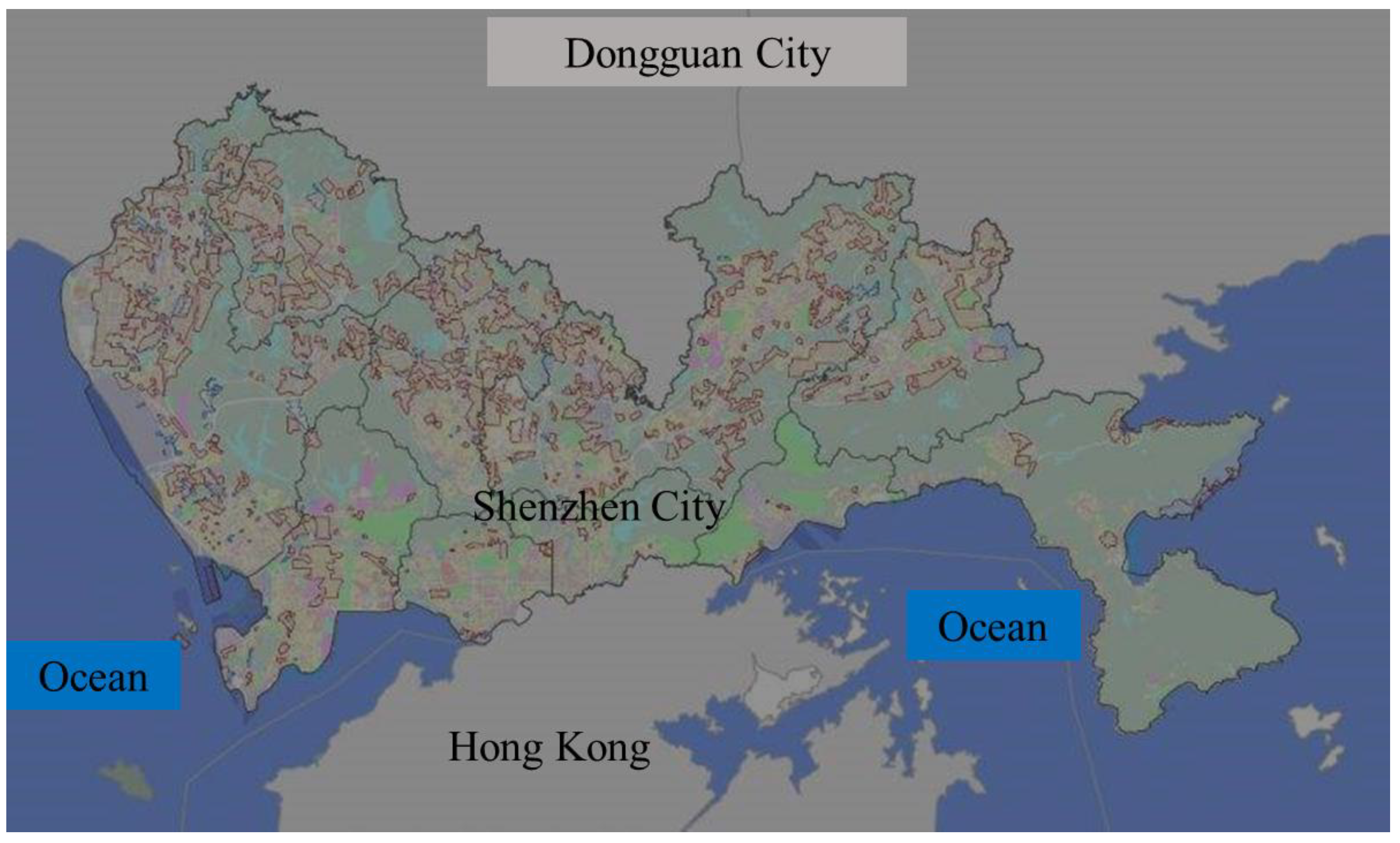
Figure 2.
Location of SXS area.

Figure 3.
Distribution of urban villages and formal residences in SXS area. (The solid circle refers to urban villages; the hollow circle refers to formal residences).
Figure 3.
Distribution of urban villages and formal residences in SXS area. (The solid circle refers to urban villages; the hollow circle refers to formal residences).
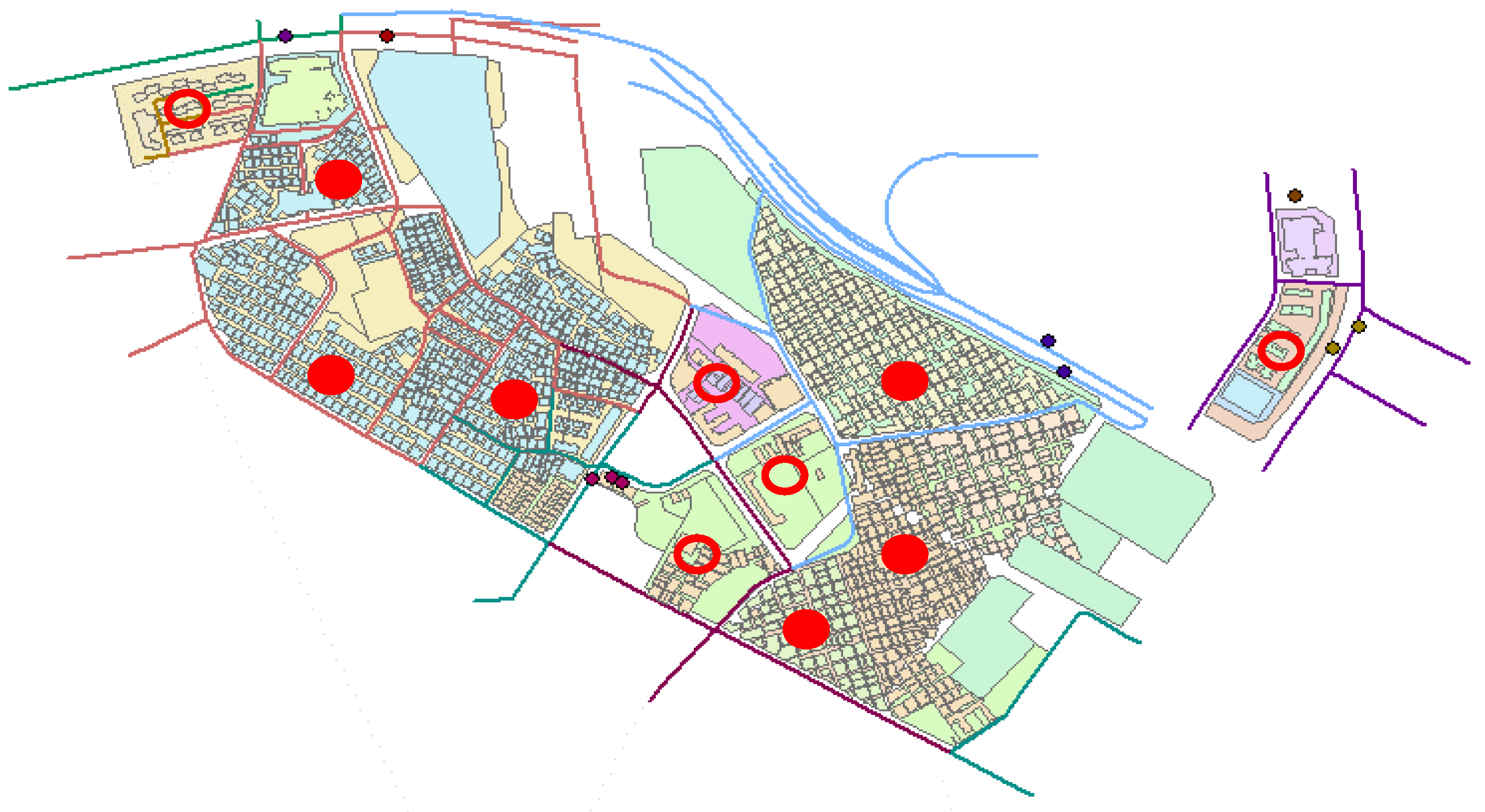
Figure 4.
Integrated database for research.

Figure 5.
Travel mode choice in urban villages and formal residences.
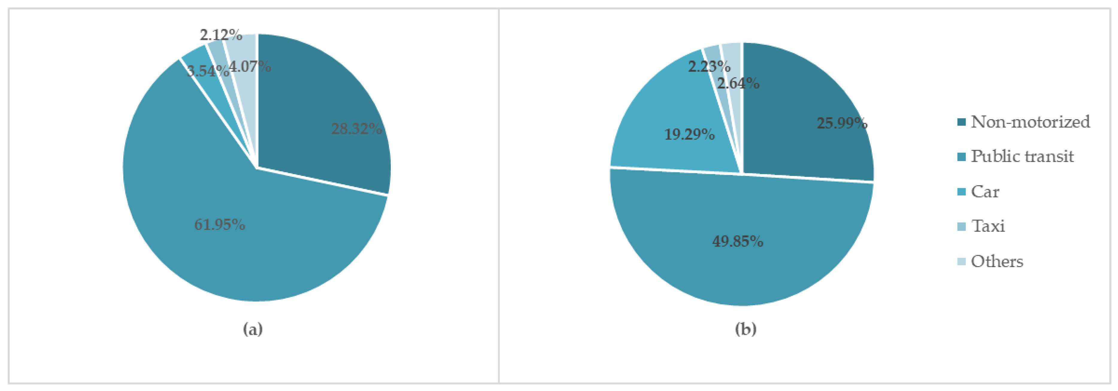
Figure 6.
Travel purpose by PT.


Table 1.
Travel characteristics comparison.
| Non-Motorised | Public Transit | Car | Taxi | Others | Total | ||
|---|---|---|---|---|---|---|---|
| 28.32 * | 61.95 * | 3.54 * | 2.12 | 4.07 | 100 | ||
| Formal residences | 25.99 * | 49.85 * | 19.29 * | 2.23 | 2.64 | 100 | |
| Travel distance (km) | Urban villages | 1.99 * | 14.77 * | 11.08 | 14.36 * | 16.85 * | 12.30 * |
| Formal residences | 2.17 * | 13.29 * | 13.40 | 5.85 * | 11.24 * | 9.87 * | |
| Travel rate 1 | Urban villages | 0.30 * | 0.78 * | 0.04 * | 0.03 | 0.05 | 1.20 * |
| Formal residences | 0.37 * | 0.72 * | 0.28 * | 0.03 | 0.04 | 1.44 * | |
* means p ≤ 0.05, ANOVA and Chi-square test show significant differences of travel features between urban villages and formal residences; 1 Travel rate means the average frequency of trips per day.
Table 2.
Socio-demographic variables profile.
| Variables | Order | Categories | Survey Data | |||
|---|---|---|---|---|---|---|
| Urban Villages (n = 565) | Formal Residences (n = 985) | |||||
| Frequency | Percentage (%) | Frequency | Percentage (%) | |||
| Gender | 0 | Female | 251 | 44.42 | 452 | 45.89 |
| 1 | Male | 314 | 55.58 | 533 | 54.11 | |
| Age | 1 | <15 | 34 | 6.02 | 114 | 11.57 |
| 2 | 15–35 | 433 | 76.64 | 687 | 69.75 | |
| 3 | 35–59 | 94 | 16.64 | 172 | 17.46 | |
| 4 | >60 | 4 | 0.71 | 12 | 1.22 | |
| Income (thousand yuan/year) | 1 | <80 | 379 | 67.08 | 244 | 24.77 |
| 2 | 80–150 | 170 | 30.09 | 681 | 69.14 | |
| 3 | 150–200 | 16 | 2.83 | 34 | 3.45 | |
| 4 | >200 | 0 | 0 | 26 | 2.64 | |
| Car ownership | 0 | No car | 535 | 94.69 | 833 | 84.57 |
| 1 | Have car | 30 | 5.31 | 152 | 15.43 | |
| Occupation | 1 | Common labour | 181 | 32.04 | 129 | 13.10 |
| 2 | High-skilled labour | 90 | 15.93 | 487 | 49.44 | |
| 3 | Self-employed | 244 | 43.19 | 234 | 23.76 | |
| 4 | Others | 50 | 8.85 | 135 | 13.71 | |
Table 3.
Other variables profile.
| Dimension | Name | Description |
|---|---|---|
| Built environment variables | Residential density | Residential density of each residential unit |
| Mixed land use | An entropy measured index 1 | |
| Distance to transit | Walking time from home to the nearest bus stop (min): 1. <5 min; 2. 5–10 min; 3. 10–20 min; 4. >20 min | |
| Bus stops | Number of bus stops within 500 m | |
| Public transit service variable | Frequency | Actual waiting time at bus stops (min): 1. <5 min; 2. 5–10 min; 3. 10–20 min; 4. >20 min |
| Daily travel features variables | Purpose | 1. Commuting; 2. Non-commuting |
| Travel distance | Distance from origin to destination (km) | |
| Travel time | Time spent during one trip (min) |
1, E refers to mixed land use (entropy); j refers to the type of land use (j = 1, 2, …, n); refers to the proportion of land use type j.
Table 4.
PT choice regression referring to non-motorised mode.
| PT Choice Variables | Urban Villages | Formal Residences | ||
|---|---|---|---|---|
| Coef. | OR | Coef. | OR | |
| Socio-demographic | ||||
| (Age = 1) | −1.707 | 0.181 | 1.944 | 6.983 |
| (Age = 2) | 1.869 | 6.480 | 3.690 *** | 40.040 |
| (Age = 3) | 1.740 | 5.696 | 2.529 ** | 12.543 |
| (Age = 4) | 0 | - | 0 | - |
| (Gender = 0) | 0.167 | 1.182 | 0.119 | 1.126 |
| (Gender = 1) | 0 | - | 0 | - |
| (Occupation = 1) | 0.200 | 1.222 | 0.783 | 2.187 |
| (Occupation = 2) | −0.063 | 0.939 | 0.564 | 1.758 |
| (Occupation = 3) | 0.658 | 1.931 | −0.036 | 0.964 |
| Occupation = 4) | 0 | - | 0 | - |
| (Income = 1) | −2.618 *** | 0.073 | −0.112 | 0.894 |
| (Income = 2) | −1.360 | 0.257 | 0.307 | 1.360 |
| (Income = 3) | 0 | - | 1.985 * | 7.280 |
| (Income = 4) | - | - | 0 | - |
| (Car ownership = 0) | 1.021 | 2.777 | 0.547 * | 1.728 |
| (Car ownership = 1) | 0 | - | 0 | - |
| Public Transit Service | ||||
| (Frequency = 1) | −0.183 | 0.833 | 0.677 | 1.968 |
| (Frequency = 2) | 0.014 | 1.014 | 0.416 | 1.516 |
| (Frequency = 3) | 0.244 | 1.276 | 0 | - |
| (Frequency = 4) | 0 | - | - | - |
| Daily Travel Features | ||||
| Travel distance | 0.150 ** | 1.161 | 0.292 *** | 1.339 |
| Travel time | 0.080 | 1.084 | 0.304 ** | 1.355 |
| (Purpose = 1) | 0.794 | 2.213 | 0.571 | 1.770 |
| (Purpose = 2) | 0 | - | 0 | - |
| Built Environment | ||||
| Bus stops | 0.020 | 1.020 | −0.175 | 0.840 |
| Residential density | −0.352 * | 0.703 | −0.454 ** | 0.561 |
| Mixed land use | −0.492 | 0.611 | 2.941 | 20.380 |
| (Distance to transit = 1) | 0.498 | 1.646 | −3.038 | 0.000 |
| (Distance to transit = 2) | 0.432 | 1.540 | −2.706 | 0.000 |
| (Distance to transit = 3) | −0.746 | 0.474 | −2.955 | 0.000 |
| (Distance to transit = 4) | 0 | - | 0 | - |
| Intercept | −0.797 | - | −33.839 | - |
*: significance < 0.1; **: significance < 0.05; ***: significance < 0.01.
Table 5.
PT choice regression referring to car mode.
| PT Choice Variables | Urban Villages | Formal Residences | ||
|---|---|---|---|---|
| Coef. | OR | Coef. | OR | |
| Socio-demographic | ||||
| (Age = 1) | 9.141 | 33.641 | −30.728 | 0.000 |
| (Age = 2) | −16.224 | 0.000 | −15.958 | 0.000 |
| (Age = 3) | −16.853 | 0.000 | −15.911 | 0.000 |
| (Age = 4) | 0 | - | 0 | - |
| (Gender = 0) | −3.278 * | 0.038 | 0.377 * | 1.458 |
| (Gender = 1) | 0 | - | 0 | - |
| (Occupation = 1) | 6.352 ** | 15.514 | −18.420 | 0.000 |
| (Occupation = 2) | 5.085 ** | 6.591 | −17.365 | 0.000 |
| (Occupation = 3) | 11.305 *** | 8.012 | −17.187 | 0.000 |
| (Occupation = 4) | 0 | - | 0 | - |
| (Income = 1) | 22.320 | 16.503 | 0.196 | 1.217 |
| (Income = 2) | 4.176 ** | 5.076 | −0.049 | 0.952 |
| (Income = 3) | 0 | - | 0.036 | 1.037 |
| (Income = 4) | - | - | 0 | - |
| (Car ownership = 0) | 1.078 | 2.938 | 2.211 *** | 9.128 |
| (Car ownership = 1) | 0 | - | 0 | - |
| Public Transit Service | ||||
| (Frequency = 1) | 13.735 | 9.471 | 0.026 | 1.027 |
| (Frequency = 2) | −0.469 | 0.626 | −0.183 | 0.833 |
| (Frequency = 3) | −1.639 | 0.194 | 0 | - |
| (Frequency = 4) | 0 | - | - | - |
| Daily Travel Features | ||||
| Travel distance | −0.115 * | 0.891 | −0.025 ** | 0.975 |
| Travel time | 6.717 *** | 16.205 | 1.366 *** | 3.922 |
| (Purpose = 1) | −15.983 | 0.000 | 0.759 | 2.137 |
| (Purpose = 2) | 0 | - | 0 | - |
| Built Environment | ||||
| Bus stops | 0.574 ** | 1.776 | 0.279 *** | 1.322 |
| Residential density | 2.278 *** | 3.103 | −0.016 | 0.984 |
| Mixed land use | −12.556 ** | 0.000 | 2.006 * | 9.593 |
| (Distance to transit = 1) | 0.561 | 1.753 | 1.577 * | 4.842 |
| (Distance to transit = 2) | 3.149 | 13.318 | 2.210 ** | 9.119 |
| (Distance to transit = 3) | 4.899 * | 14.156 | 1.616 | 5.032 |
| (Distance to transit = 4) | 0 | - | 0 | - |
| Intercept | 26.806 | - | 7.293 | - |
*: significance < 0.1; **: significance < 0.05; ***: significance < 0.01.
© 2018 by the authors. Licensee MDPI, Basel, Switzerland. This article is an open access article distributed under the terms and conditions of the Creative Commons Attribution (CC BY) license (http://creativecommons.org/licenses/by/4.0/).
Share and Cite
MDPI and ACS Style
Yu, L.; Xie, B.; Chan, E.H.W. How does the Built Environment Influence Public Transit Choice in Urban Villages in China? Sustainability 2019, 11, 148. https://doi.org/10.3390/su11010148
AMA Style
Yu L, Xie B, Chan EHW. How does the Built Environment Influence Public Transit Choice in Urban Villages in China? Sustainability. 2019; 11(1):148. https://doi.org/10.3390/su11010148
Chicago/Turabian StyleYu, Le, Binglei Xie, and Edwin H. W. Chan. 2019. "How does the Built Environment Influence Public Transit Choice in Urban Villages in China?" Sustainability 11, no. 1: 148. https://doi.org/10.3390/su11010148
Note that from the first issue of 2016, this journal uses article numbers instead of page numbers. See further details here.