Short-Term Wind Power Forecasting: A New Hybrid Model Combined Extreme-Point Symmetric Mode Decomposition, Extreme Learning Machine and Particle Swarm Optimization

Abstract

The nonlinear and non-stationary nature of wind power creates a difficult challenge for the stable operation of the power system when it accesses the grid. Improving the prediction accuracy of short-term wind power is beneficial to the power system dispatching department in formulating a power generation plan, reducing the rotation reserve capacity and improving the safety and reliability of the power grid operation. This paper has constructed a new hybrid model, named the ESMD-PSO-ELM model, which combines Extreme-point symmetric mode decomposition (ESMD), Extreme Learning Machine (ELM) and Particle swarm optimization (PSO). Firstly, the ESMD is applied to decompose wind power into several intrinsic mode functions (IMFs) and one residual(R). Then, the PSO-ELM is applied to predict each IMF and R. Finally, the predicted values of these components are assembled into the final forecast value compared with the original wind power. To verify the predictive performance of the proposed model, this paper selects actual wind power data from 1 April 2016 to 30 April 2016 with a total of 2880 observation values located in Yunnan, China for the experimental sample. The MAPE, N_MAE and N_RMSE values of the proposed model are 4.76, 2.23 and 2.70, respectively, and these values are lower than those of the other eight models. The empirical study demonstrates that the proposed model is more robust and accurate in forecasting short-term wind power compared with the other eight models.

1. Introduction

The utilization of renewable energy is one of the world’s hot topics. As an essential component of renewable energy, wind energy is an environmentally friendly clean energy and its development has been highly valued by all countries including China. In recent years, under the guidance and motivation of renewable energy law, the policy of energy-saving and emission-reduction in China, new energy power generation is burgeoning, especially wind power, and the account for the proportion of low valley load capacity has increased. However, it can seriously affect the quality of the grid power and the operation of the power system when the proportions of wind power in the network load more than a certain value. Simultaneously, the characteristics of instability and volatility also have an unbearable impact on the power system. The most effective way to conquer the shortcomings is to forecast wind power, so that the electric power dispatching departments can ensure the safety of the power balance of the power grid according to the change in wind power.

As for wind power prediction, there are different partitions on the basis of different scales. The prediction time scale can be divided into long-term forecast, medium-term forecast and short-term prediction. Meanwhile, according to the prediction of physical quantities, it can be roughly divided into two categories: a direct method and an indirect method [1]. The first category, which can be called the statistical model, is to forecast the wind power directly; this method has a strong dependency on the input data and is based on the assumption that linear structures exist among time series. Faghani et al. exploited the extrapolation methods to robustly determine wind speed and wind power density at higher altitudes, which can be extrapolated to the wind speeds data at any heights within any geographical region [2]. In order to overcome the limitations of the individual forecasting models, Song et al. built a combined model with the theory of a data preprocessing technique, forecasting algorithms, advanced optimization algorithm, and no negative constraint [3]. Han et al. investigated historical wind power data and used Phase Space Reconstruction (PSR), Principle Component Analysis (PCA) and Resource Allocating Network (RAN), respectively, to analysis the wind power [4]. With the aim of demonstrating the effect of the proven model, the study made a comparison with Persistence (PER), New-Reference (NR), and Adaptive Wavelet Neural Network (AWNN) models.

Jiang and Huang improved the real–time decomposition-based forecasting method; at the same time, they used feature selection and error correction to enhance the performance of the model and the prediction accuracy [5]. Oktay et al. believed that the wind speed time series has non-linear characteristics, then, the study adapted Polynomial AR (PAR) models to make power predictions, and compared the differences between PAR and artificial neural network adaptive neuron fuzzy inference system (ANN-ANFIS) models [6]. Ilhami et al. developed the moving average (MA), weighted moving average (WMA), autoregressive moving average (ARMA) and autoregressive integrated moving average (ARIMA) methods to forecast wind speed and wind power at different time horizons [7]. Zhao et al. proposed a self-adaptive (SA) and an auto-regressive integrated moving average (ARIMAX) optimized by a chaotic particle swarm optimization (CPSO) algorithm, which can be called the SA-ARIMA-CPSO approach, to predict wind speed. It concluded that the hybrid model has the best performance compared with several other models [8]. Maatallah et al. made a comparison between the Hammerstein model and an Autoregressive (HAR) approach with a classical Autoregressive Integrated Moving Average (ARIMA) model and a multi-layer perception Artificial Neural Network (ANN), and the results show that the HAR model is beneficial for wind speed forecasting [9]. Kavasseri and Seetharaman employed fractional-ARIMA (f-ARIMA) models to forecast wind speeds on the day-ahead (24 h) and it concluded that the model significantly improves the accuracy of forecasting wind power [10]. Aiming to solve the nonlinearity and uncertainty problems of linear autoregressive integrated moving average (ARIMA) model, Shukur and Lee used an artificial neural network (ANN) and Kalman filter (KF) to optimize ARIMA, and established a hybrid KF-ANN model [11].

The principle of second category, which can be called physical methods, is to forecast wind power according to varied parameters; however, the prediction accuracy of this method is mainly restricted by wind speed. At the same time, it will be affected by many factors such as temperature, and humidity, and prediction accuracy is limited. Francis et al. evaluated the use of Soil Moisture Ocean Salinity (SMOS) wind speeds within Met Office numerical weather prediction (NWP), and provide information on the ocean surface wind speed under high wind and rain conditions [12]. Based on Numerical Weather Prediction (NWP) models, Allena et al. predicted long-term wind speeds with the boundary layer scaling (BLS) method, and the result indicated that using the BLS model for wind speed and NWP data for power density predictions has advantages. There are also intelligent methods, such as artificial neural network methods; these methods are suited to predicting over a shorter time scale. It is known that nonlinear prediction methods such as artificial neural networks (ANN) and adaptive neuron fuzzy inference systems (ANFIS) perform better than linear autoregressive (AR) and AR moving average models [13]. Niu et al. proposed an artificial neural network and optimized it with a modified bat algorithm with cognition strategy to effectively predict wind power. The study indicated that the model can remedy the deficiencies of artificial neural networks [14]. Li and Shi utilized three types of neural networks including adaptive linear element, back propagation and radial basis function, to observe the hourly mean wind speed. It reflected that the reliablity of wind speed forecasting depends on data sources and models [15]. Madhiarasan and Deepa developed an artificial neural networks (ANN) model to prove that the model can enhance the accuracy rate, reduce error and converge fast. At the same time, it also proved the applicability of ANN [16]. Due to the random fluctuations of wind speed, Kadhem et al. applied the hybrid artificial neural network (HANN) to ensure the accuracy of forecasting [17].

However, each method has its own inherent defects in forecasting wind power including the high accuracy and strong stability of the method. Thus, with the aim of taking the advantages and overcoming the shortages of each model, many combined wind speed forecasting methods have been put forward. Zheng et al. proposed a flexibility and efficiency model, which uses a composite quintile regression outlier-robust extreme learning machine and a hybrid population-based algorithm to explore the characteristics of wind speed variables while also improving model robustness and predictive capability [18]. Wang et al. developed a novel combined forecasting model consisting of four artificial neural networks and incorporated the MOBA (multi-objective bat algorithm) and data decomposition [19]. Hu, Wang, and Xiao used the Empirical Wavelet Transform (EWT), Expectation Propagation (EP) algorithm and Gaussian process regression with the Student-t Observation Model (GPR-t) to study the dynamic characteristics of wind speed [20]. Yu, Li, and Zhang adopted Improved WT (IWT) and Singular Spectrum Analysis (SSA) to preprocess the options and designed a model combined with the IWT-ENN and Elman Neural Networks (ENN) [21]. Liu et al. employed Wavelet Decomposition-WD, Wavelet Packet Decomposition-WPD, Empirical Mode Decomposition-EMD and Fast Ensemble Empirical Mode and Decomposition-FEEMD to decompose the influence factors, and proposed the model of FEEMD-MLP and FEEMD-ANFIS to improve the forecast precision of wind speed [22]. Compared with the BP model, the WPD-BP model, the WPD-CEEMDAN-BP model, the RBF model, the WPD-RBF model, the WPD-CEEMDAN-RBF model, the GRNN model, the WPD-GRNN model and the WPD-CEEMDAN-GRNN model, Liu et al. established a new hybrid framework, which was based on WPD (Wavelet Packet Decomposition), the CEEMDAN (Complete Ensemble Empirical Mode Decomposition) and the ANN (Artificial Neural Network). The study indicated that the new hybrid model performed better [23]. Li et al. took advantage of the EWT-LSTM-RELM-IEWT model and validated the forecasting capacity of the proposed hybrid [24]. Han et al. explored and compared the hybrid autoregressive moving average non-parametric and hybrid non-parametric autoregressive moving average models, and this study indicated that the non-parametric based hybrid models generally outperform the other models and have more robust forecast performances [25]. For averting the drawback of weak generalization capability and robustness of a single approach, Chen et al. proposed a novel method called Ensem LSTM, which uses a nonlinear-learning ensemble of deep learning time series prediction based on LSTMs (Long Short Term Memory neural networks), SVRM (support vector regression machine) and EOA (external optimization algorithm) [26]. Niu et al. (2018) adopted a preprocessing module, a feature selection module, an optimization module, a forecast module and an evaluation module, respectively, to select the optimal input and predict the wind speed. The current research is focused on improving the precision of short-term power. Machine learning (ML) is one of the core research areas of artificial intelligence and neural computation [27]. Using a wind speed time series, Santamaría-Bonfil et al. conducted training on a Support Vector machine (SVM), and forecast the wind speed with the Time Delay Coordinates model. Compared with autoregressive models (AR, ARMA, and ARIMA) tuned by Akaike’s Information Criterion and the Ordinary Least Squares method. The results verified the accuracy of the hybrid methodology [28]. Based on Hybrid Ensemble Empirical Mode Decomposition (EEMD) and Least Square Support Vector Machine (LSSVM), Tan et al. predicted short-term wind speed. Subsequently, the study compared the model with LSSVM, Back Propagation Neural Networks (BP), Auto-Regressive Integrated Moving Average (ARIMA), combination of Empirical Mode Decomposition (EMD) with LSSVM, and hybrid EEMD with ARIMA models [29]. Combining the methods of the multi-step wind speed forecasting based on Wavelet Domain Denoising, Wavelet Packet Decomposition, Empirical Mode Decomposition, Auto Regressive Moving Average, Extreme Learning Machine and Outlier Correction Method, Mi, Liu, and Li decomposed the factors of wind speed forecasting twice; finally, the study estimated the performance of the new method [30]. Zhang et al. established a compound structure of extreme learning machine (ELM) with hybrid backtracking search algorithm (HBSA); the real-valued BSA (RBSA), partial autocorrelation function (PACF), optimized variation mode decomposition (OVMD), and the residual evaluation index (REI) provided an effective hybrid model to forecast wind power [31]. Based on the WPD (Wavelet Packet Decomposition), the EMD (Empirical Mode Decomposition) and the ELM (Extreme Learning Machine), Liu, Mi, and Li built a combined forecasting method and compared it with the PM (Persistent Model), the ARIMA model, the SVM model, the ELM model, the WPD-ELM model, the WPD-EMD (LF)-ELM model, the WPD-EMD (HF)-ELM model and the WPD-EMD-ELM model [32].

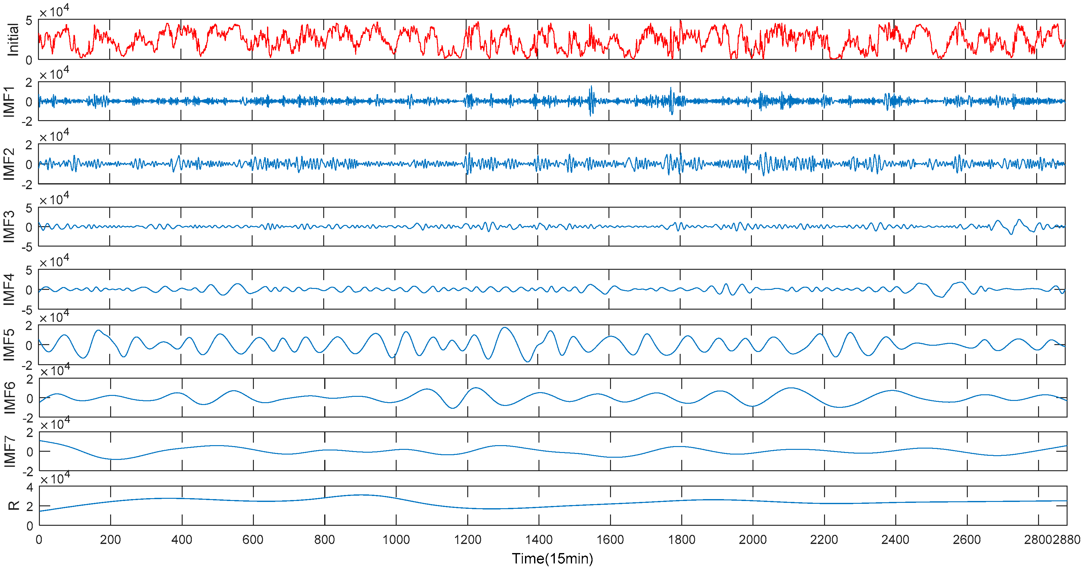
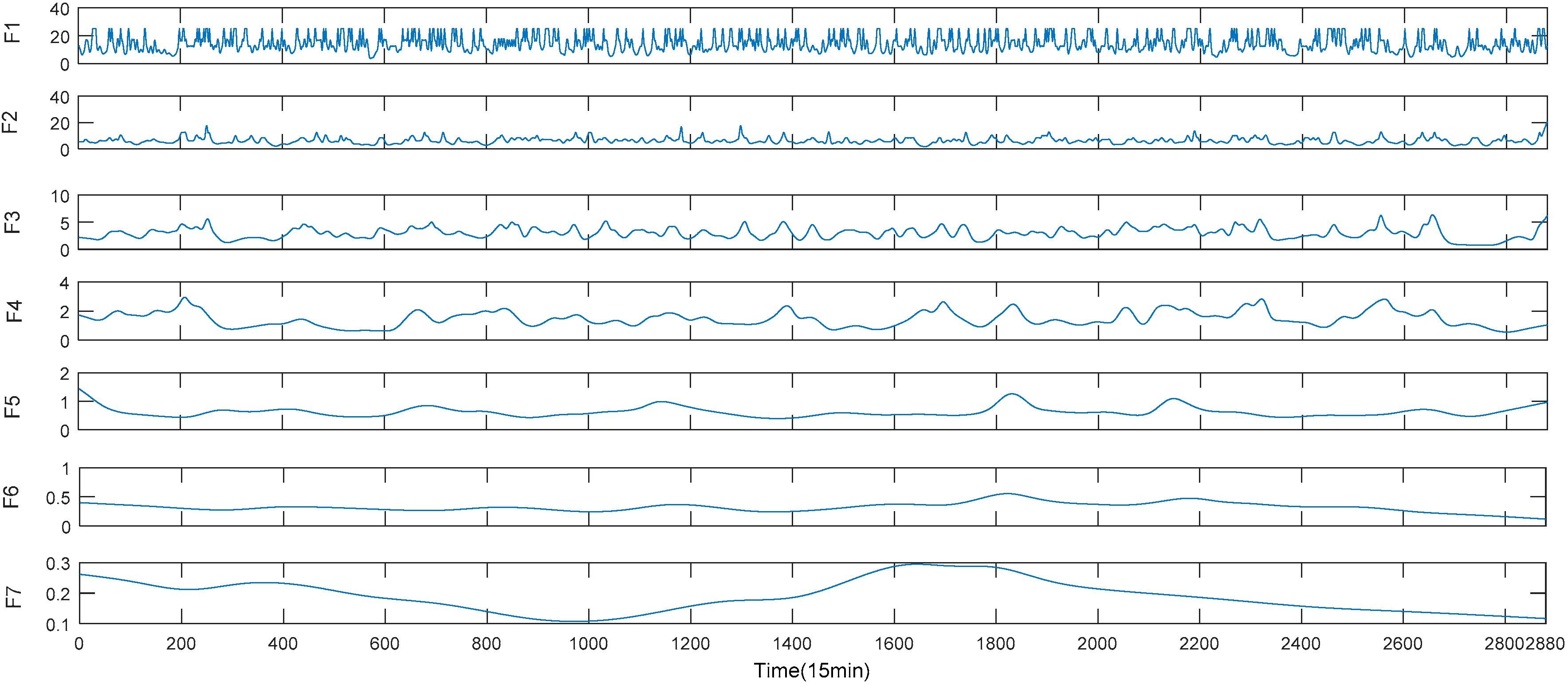
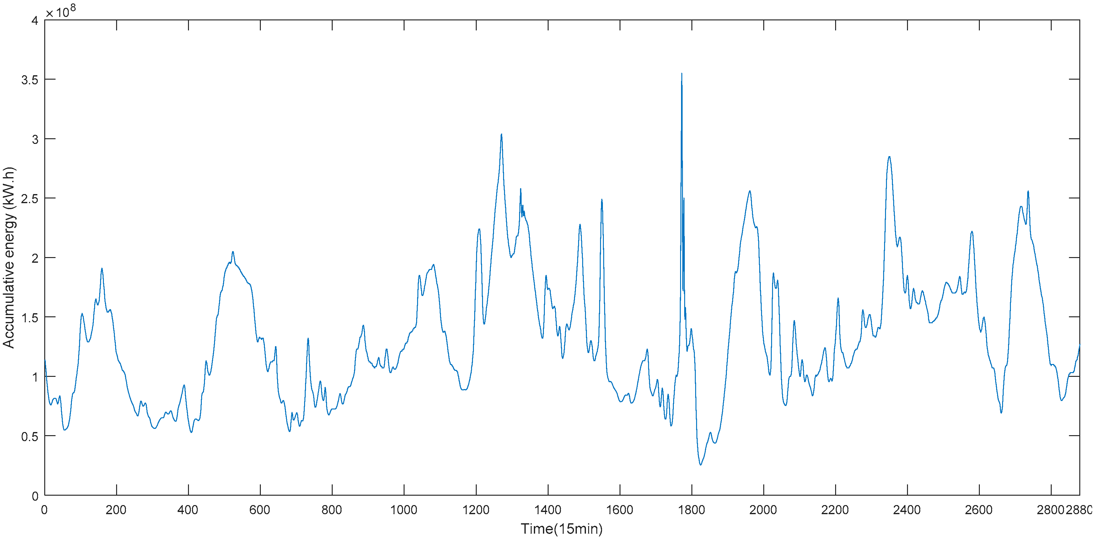
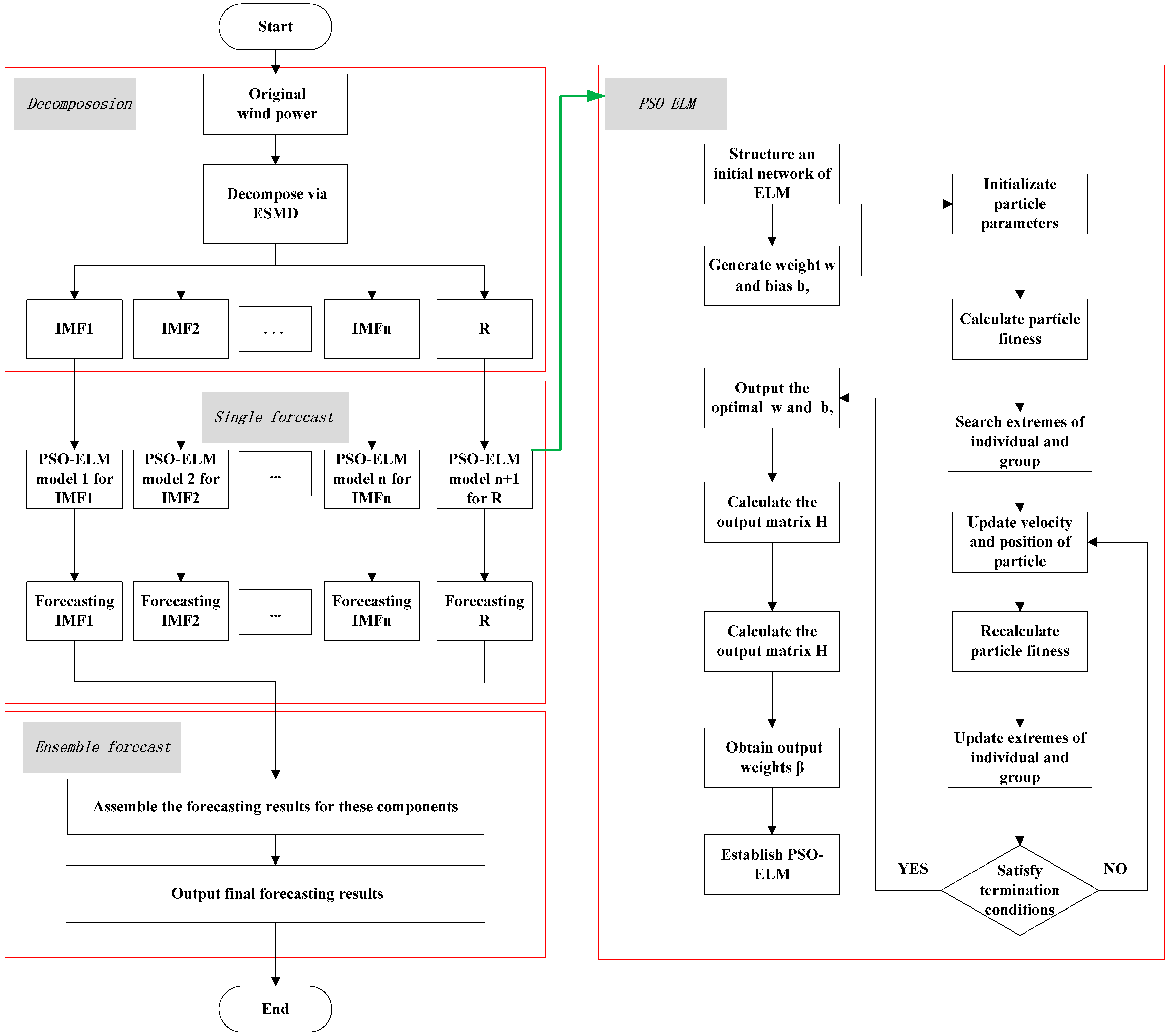
Given the great significance of short-term power prediction for electric power dispatching and taking into account the characteristics of wind speed time series, this paper constructed a new hybrid model, the ESMD-PSO-ELM model. ESMD has better adaptive processing characteristics for nonlinear and non-stationary time series. Among these, a direct interpolation (DI) method is used for ESMD and this method directly depicts the frequency and amplitude variability of each component. This method can also intuitively reflect the total energy with time-variation. ELM has the advantage of training fast, high fitting precision and good generalization performances. The PSO algorithm has the characteristics of a simple algorithm, strong robustness and fast convergence. The combined model can not only reduce the running time of the model, but also increase the accuracy of the results.

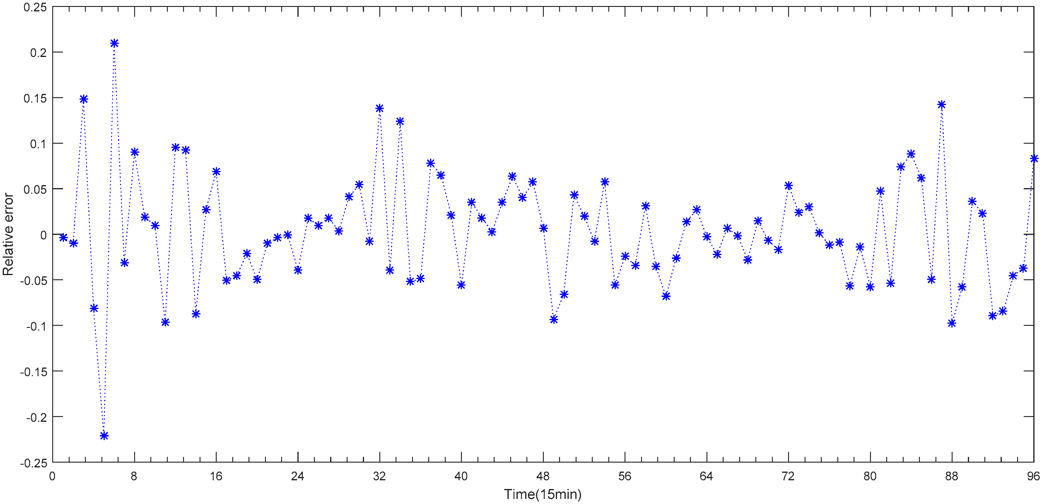
This paper is structured as follows: Section 2 discusses the ESMD, ELM and PSO, respectively; Section 3 introduces the flow chart of ESMD-PSO-ELM model; the empirical analysis is conducted in Section 4; Section 5 analyzes the prediction results of short-term wind power; Conclusions are presented in Section 6.

2. Methods

2.1. EMD Algorithm

Empirical mode decomposition (EMD) is an efficient and adaptive analysis method for handling nonlinear and non-stationary time series data. This method decomposes the original signal with a large amount of information into simple components at different scales and frequencies via iterative steps [33]. Each simple component serves as an IMF, which needs three prerequisites: (a) there are at least two extremes in the original signal, namely, a maximum value and a minimum value; (b) the characteristic time scale in the original signal is determined by the time length between the two extremes; (c) the original signal can be derived from the extreme value by the difference if only inflection points. The detailed EMD procedure is briefly expressed in Algorithm 1:

Algorithm 1. Empirical mode decomposition (EMD) Algorithm

Step 1: Mark the original signal as time series $x(t)$, Identify all the maxima and minima of $x(t)$ and generate its upper and lower envelopes, $a(t)$ and $b(t)$, via cubic spline interpolations.

Step 2: Compute the mean values $m(t)$ of the envelopes. ($m(t)=\left[a(t)+b(t)\right]/2$).

Step 3: Calculate the difference ($c(t)=x(t)-m(t)$).

Step 4: Check the properties of $c(t)$. If $c(t)$ cannot satisfy the two criteria of the IMF, let $x(t)=c(t)$, and return to the step 1; otherwise, $c(t)$ is defined as an IMF, and let the residual $r(t)=x(t)-c(t)$.

Step 5: Repeat steps 1–4 only when the termination criterion is satisfied.

Step 6: The x(t) can be reconstructed as follows: $x(t)={\displaystyle \sum _{i=1}^n{c}_i}(t)+r(t)$

2.2. ESMD Algorithm

Extreme-point symmetric mode decomposition (ESMD) is a nonlinear time-varying signal decomposition method that is data driven, which has better adaptive processing characteristics for nonlinear and non-stationary time series [34]. This algorithm is developed on the basis of the EMD. It determines that the spline interpolation of the outer envelope in the EMD is changed to the internal pole symmetric interpolation. It utilizes the least square method to optimize the intrinsic mode in order to extend it from local adaptation to global adaptation and iterate to generate the best number of filters. The method effectively solves the problem of frequency crossover in EMD. In view of the inherent defects of some classical time-frequency transform methods, a direct interpolation (DI) method is used for ESMD and the method directly depicts the frequency and amplitude variability of each component. It completely changes the theory of spectrum analysis of integral transformation. The detailed ESMD procedure is briefly expressed in Algorithm 2:

Algorithm 2. Extreme–point symmetric mode decomposition (ESMD) Algorithm

Step 1: Find all of the local extreme points included maximum points and minimum points of time series X(t), and then label them as Ei with 1 ≤ i ≤ n.

Step 2: Calculate all of the adjacent poles Ei and mark the midpoints by Fi with 1 ≤ i ≤ n − 1.

Step 3: Add a left boundary midpoint F0 and a right boundary midpoint Fn through a direct interpolation.

Step 4: Construct p interpolating curves L1, …, LP (p ≥ 1) though the n + 1 midpoints and calculate the mean value L* = (L1 + … + LP)/p.

Step 5: Repeat the step 1–step 4 about X(t) − L* until |L*| ≤ ε (ε is called a permitted error) or the shifting times gain a pre-set maximum number K. And then the first mode M1 is produced.

Step 6: Repeat the step 1–step 5 about X(t) − M1 and gain M2, M3 … until the last residual R has no more than a certain number of extreme points.

Step 7: Alter the maximum number K and repeat the step 1–step 6 and then calculate standard deviation σ of X(t) − R when K takes different values.

Step 8: Find the K corresponds to a minimum σ and gain the corresponding mode M1, …, R, which are used as the decomposition result.

The explanations for the key steps in view of the ESMD algorithm are as follows: In Step 4, the ESMD has three main forms of ESMD_I, ESMD_II, ESMD_III according to the difference of P number and the form of this article is ESMD_II [35]. In Step 5, the permissible error ε and the maximum number K need to be set in advance.

The formula of data standard deviation ${\sigma }_0$:

$${\sigma }_0=\frac{1}{N}{\displaystyle \sum _{i=1}^N}{(x_i-\overline{X})}^2$$

(1)

wherein, N is the number of sampling points; X_i is the value of the ith sampling point; $\overline{X}$ is the average value of the data.

The formula of numerical definition $\sigma$:

$$\sigma =\frac{1}{N}{\displaystyle \sum _{i=1}^N}{(x_i-r_i)}^2$$

(2)

The fitting Degree $\sigma$ is the ratio of (1) and (2), which reflects the trend change of the trend term and the original signal. If the value is smaller, the decomposition result is better. In Step 6, the number of residual points is set at least 4 poles because modal oscillation characteristics are shown for at least 2 poles and modal oscillations repeated at least 2 times are shown periodically. Nevertheless, the set value cannot be too big in order to avoid the modality omission.

2.3. ELM and PSO Algorithm

Extreme Learning Machine (ELM) was proposed as a new type of single-hidden-layer feed forward neural network (SLFN) by Huang et al. [36]. The network is simple and efficient and it only needs to set the number of hidden layer nodes. The network randomly generates the connection weights between the input layer and the hidden layer and the output weights between the hidden layer and the output layer are acquired via the least squares method using the minimizing squared loss function. The advantage of ELM is the fast training speed, high fitting precision and good generalization performances. At the same time, it overcomes the disadvantages of long learning time and the susceptibility to easily fall into local minimum. It has been widely used in many fields.

Particle swarm optimization (PSO), proposed by Kennedy and Eberhart [37], is a stochastic optimization algorithm that simulates the social behavior of biological organisms such as birds [38]. For particle optimization, the solution of every optimization problem is like a bird in search space, which is called a particle. Each particle has initialization speed and initialization location, the fitness value determined by fitness function. Each particle is given a memory function that can search the best position; moreover, the velocity of each particle determines the direction and distance of their flight so that the particles can be searched for in the optimal solution space.

As a random search and parallel optimization algorithm, the PSO algorithm has the characteristics of a simple algorithm—strong robustness and fast convergence. The algorithm is good at finding the global optimal solution of the problem with large probability. In this paper, the PSO algorithm is used to optimize the weight $w$ and bias. $b$ of ELM, to establish the short-term prediction model of wind power.

The procedure of PSO-ELM is briefly described in Algorithm 3.

Algorithm 3. Particle swarm optimization–extreme learning machine (PSO-ELM) Algorithm

Step 1: Preset training set, $N=\{(x_i,y_i)\}|x_i\in R^n,y_i\in R,i\in [1,m]$ with the activation function g(x), and the number of hidden layer neurons $N$

Step 2: Generate random values for the weight $w_i$ and bias $b_i$,$i\in [1,N]$

Step 3: Initialize the particle swarm, and randomly set the population, position and velocity of each particle.

Step 4: Calculate the fitness and update the velocity and the position parameters.

Step 5: Output the optimal $w$ and $b$ parameters.

Step 6: Calculate the hidden layer output matrix, H,

$H=\left[\begin{array}{ccc}g(w_1{x}_1+b_1)& \cdots & g(w_N{x}_1+b_N)\\ g(w_1{x}_2+b_1)& \cdots & g(w_N{x}_2+b_N)\\ ⋮& \cdots & ⋮\\ g(w_1{x}_N+b_1)& \cdots & g(w_N{x}_N+b_N)\end{array}\right]$

Step 7: Calculate the output weight, $\beta =H^{†}Y$, wherein $H^{†}$ is Moore-Penrose pseudo inverse and the label matrix of the training set is $Y={\left[y_1,y_2,\cdots ,y_N\right]}^T$

Step 8: Obtain output weights, $\beta$

3. ESMD-PSO-ELM Model

The paper proposes a hybrid prediction model based on the ESMD algorithm (ESMD-PSO-ELM) to forecast short-term wind power. ESMD is used to decompose an original sequence into several subseries and then the PSO-ELM is used to forecast each subseries according to their characteristics. This flow chart of the ESMD-PSO-ELM model is as shown in Figure 1. The model comprises following key steps: First, each nonlinear and non–stationary wind power sequence is decomposed into several stable regular IMFs and one residual via ESMD algorithm. Then, the PSO-ELM is applied to predict each IMF and one residual R. Finally, the predicted values of these components are assembled into the final forecast value compared with the original wind power.

4. Empirical Analysis

4.1. Data Selection

In order to verify the availability and practicability of the proposed model, the paper selects wind power data from site A, a wind farm located in Yunnan, China. The rated installed capacity of the wind farm is 49.5 MW. The climate type in this area is the north subtropical north plateau monsoon and the altitude of the wind farm is between 2100 m and 2370 m. This area has abundant wind energy resources due to its particular favorable terrain and the influence of atmospheric circulation. In this paper, the experimental data chooses is 15 min wind power data from 1 April 2016 to 30 April 2016 with a total of 2880 observation values. It is shown in Figure 2 and

Table 1. The statistical descriptions of wind power.

Sample	Mean	Std. Dev	Median	Maximum	Minimum	Skewness	Kurtosis
2880	23,704.88	11,674.68	24,512.06	48,323.11	111.11	−0.14	−0.98

. The wind power sequence has non–stationary and nonlinear characteristics.

4.2. Determine the Number of Screening

ESMD is applied to analyze wind power sequence. The best screening number is determined before the sequence decomposition. After repeated tests and comparisons, the number of remaining extreme points of wind power is 15 and the number of iterations is 40. The minimum value of the variance ratio corresponds to the 29th time and is shown in Figure 3.

4.3. Analysis of the IMFs

After setting the best number of screening time, the original sequence is divided into seven IMFs and one residual via ESMD. Then the frequency and amplitude fluctuations of each component are plotted separately. The purpose is to compare the variation of time frequency and amplitude at the same time. The decomposition is shown in Figure 4. The frequency and amplitude is shown in Figure 5 and Figure 6.

Each IMF decomposed by ESMD method is independent from every other. Overall, the frequency fluctuation range gradually decreases from F1 to F7. The amplitude fluctuation range increases from A1 to A5 and declines from A6 to A7. From the point view of each IMF, the frequency of A1 and A2 changes rapidly vary from 5 to 30 Units. The IMF1 and IMF2 show a very short interval time and almost without periodicity, which belongs to a short-term trend. However, the amplitude of F1 and F2 varies very little in the original sequence, which belongs to the local intense shock of the curve. These changes should be mainly associated with meteorological factors. The frequency of F6 and F7 changes slightly, the value of which remains less than 1 Units. And there are quite long time intervals between adjacent extreme points. The IMF6, IMF7 and trend R are associated with the medium or long–term trend of the original sequence. Though the amplitude fluctuations of A6 and A7 are small, they occupy a large proportion in the original sequence. These changes should be mainly related to national macroeconomic regulation policy and national economic development. The frequency of A3, A4 and A5 changes slowly and it has certain regularity. These components make up the medium–term trend in the original sequence. However, the amplitude variation of F5 is the largest of all components and the curve trend of IMF5 is closest to the original sequence. The IMF3, IMF4 and IMF5 mainly reflect the regional power grid regulation policies and the local economy.

In summary, the stability of the sequence from IMF1 to IMF7 gradually becomes stronger and the fluctuation situation decreases steadily. The IMFs with great frequency variation have a small proportion in the original sequence, that is to say, the violent oscillation of the high-frequency part will not affect the overall trend of the original sequence. In contrast, the low frequency part with a smooth and stable trend has a large proportion of the original sequence. It can be shown that the IMFs are more stable than the original signal sequence through ESMD and hence is more conducive to the acquisition of signal information characteristics and the prediction of the nonlinear and nonstationary sequences.

4.4. Analysis of AGM

The adaptive global mean (AGM) line is the unique decomposition product of HHT theory. In the process of decomposition, the curve is adaptively decomposed according to the sequence curve of the original signal. As shown in Figure 7, this curve depicts the general trend of the original sequence over this period. Although it is difficult to find an inherent law in the wind power curve, the corresponding adaptive global mean is a stable curve with periodic regularity. AGM shows the overall trend of wind power and the situation of its trend changes. According to the relevant literature, the corresponding value of AGM is close to that of trend R. The study of trend R and AGM can better predict wind power more effectively and therefore improve the overall prediction accuracy.

4.5. Analysis of Accumulative Energy

In this paper, time-frequency analysis is used to characterize the accumulative energy time series of wind power series. Figure 8 well reflects the trend line of energy accumulation for IMFs and trend R at the corresponding time. Among them, the number of points corresponding to the peak points is not large. It is further explained that the wind power via the ESMD is very effective. The most drastic change of the peak points is mainly between the 1200th and 2000th sample points, which also confirm the volatility of IMFs in this area. The purpose is to prepare for the next prediction method selection and the fitting accuracy evaluation.

5. Short-Term Wind Power Forecasting

The main procedures in the paper were performed in the MATLAB R2015b environment, running on the Windows 7 system. The prediction experiments of short-term wind power were carried out based on the establishing evaluation criteria and comparison models, which verified the practicability and effectiveness of the proposed hybrid model.

5.1. Model Performance Evaluation

In general, performance measures—the mean absolute percentage error (MAPE), the mean absolute error (MAE), and the root mean square error (RMSE)—are usually applied. Among these, the MAPE is mean value of relative distance at each data point, the MAE shows the average distance between the actual value and the predicted value, the RMSE is a quadratic scoring rule estimating the average magnitude of error. To quantitatively examine the prediction performances of the proposed hybrid model, the paper needs to normalize the MAE and RMSE.

Improved performance measures for the wind power prediction model named N_MAE and N_RMSE [39]. The smaller MAPE, N_MAE and N_RMSE values indicate lower deviations of the prediction value from the actual values. The algorithms are shown in Equations (3)–(5).

$$\mathrm{MAPE}=\frac{1}{n}{\displaystyle \sum _{t=1}^n\left|\frac{y_t-{\stackrel{⌢}{y}}_t}{y_t}\right|}\times 100\%$$

(3)

$${\mathrm{N}}_{\mathrm{MAE}}=\frac{1}{P_{c}n}{\displaystyle \sum _{t=1}^n\left|y_t-{\stackrel{⌢}{y}}_t\right|}\times 100\%$$

(4)

$${\mathrm{N}}_{\mathrm{RMSE}}=\sqrt{\frac{1}{P_{c}n}{{\displaystyle \sum _{t=1}^n\left|y_t-{\stackrel{⌢}{y}}_t\right|}}^2}\times 100\%$$

(5)

wherein, P_c is the rated installed capacity of site A wind farm, $y_t$ is the t-th actual values, ${\stackrel{⌢}{y}}_t$ is the t-th prediction value, n represents the number of evaluated data points.

5.2. The Comparison Models

The paper adopts three kinds of prediction models combined with three data processing methods, which are showed in Figure 9 in detail. The ESMD-PSO-ELM is the proposed hybrid model, which compares to other eight models. The purpose is to verify the validity of the proposed hybrid model.

5.3. Parameter Setting and Input Selection

In this paper, the three prediction models, PSO-ELM, ELM and BPNN, were applied. In PSO, the initial population size was set to 40, the max-generation was 100 and the mutation probability was set to 0.6. Moreover, the range of the variance was [−5, 5], and the velocity range was [−1, 1]. In ELM, the number of hidden layer nodes was between 10 and 30 according to the characteristics of IMFs and R. In BPNN, the maximum number of training was 1000, the learning rate was 0.01, the training requirement accuracy was 0.001 and the number of neurons in the hidden layer was 9. The experimental data were a total of 2880 points—the wind power data. Among these, the first 2784 points of IMFs and R were selected as the training sample to establish the prediction model while the rest of the 96 points of IMFs and R were employed for testing. The data statistical description of wind power is shown in

Table 2. The statistical description of wind power data.

Label		Size	Maximum	Minimum	Mean	Std. Dev.
Train data	IMF1	2784	15,218.20	−14,149.83	30.48	2421.54
	IMF2	2784	15,158.62	−14,441.81	−7.73	2988.16
	IMF3	2784	19,802.86	−22,281.22	18.33	4108.04
	IMF4	2784	15,156.57	−15,907.55	−64.77	4470.38
	IMF5	2784	18,156.85	−17,473.82	8.18	6998.89
	IMF6	2784	10,152.59	−11,261.46	132.31	3702.37
	IMF7	2784	6857.93	−7069.60	3804.15	66.14
	IMF8	2784	3584.14	−3900.91	−190.48	2140.34
	R	2784	24,562.71	22,723.71	23,587.10	634.43
Test data	IMF1	96	3948.54	−3405.46	−43.06	1577.14
	IMF2	96	6886.71	−6715.46	−98.93	2557.48
	IMF3	96	8816.44	−11,719.07	−484.03	5301.74
	IMF4	96	12,397.51	−12,679.34	−2649.74	6803.399
	IMF5	96	2406.28	−1626.55	277.73	1385.30
	IMF6	96	365.64	−1.06	253.07	97.24
	IMF7	96	4468.50	1146.62	3309.66	1036.19
	IMF8	96	2872.25	2162.35	2562.75	209.91
	R	96	24,280.99	24,139.06	24,212.46	41.67

. The paper adopts the PSO-ELM to predict each IMF and one residual R and then the predicted values of these components are assembled into the final forecast value compared with the actual value.

5.4. Forecast Results

The relative errors of the proposed hybrid model are depicted in Figure 10. It is relatively stable, generally ranging between plus and minus 0.1. Moreover, the relative errors of four points are between 0.1 and 0.15 and only two points have an absolute value of relative error greater than 0.2. This indicates that the proposed model has high accuracy in forecasting short-term wind power. Figure 11 shows the fitting curves of short-term wind power for nine models. The following conclusions can be drawn: the hybrid model proposed by ESMD-PSO-ELM has the best prediction accuracy and the lowest prediction error between the actual value and predicted value. The EMD-PSO-ELM, the ESMD-ELM, and the EMD-ELM performances are very good on fitting degree, while single prediction models including BPNN and ELM have a poor prediction performance. Among all the models, the BPNN model shows the lowest performance compared with other models because the inherent characteristics may lead to low efficiency and local optimums. Moreover, the selection of the hidden nodes of BPNN depends on trial and error procedures, making it difficult to obtain an optimal network that can improve prediction performance. In a word, the hybrid models have better prediction accuracy than single form models. Decomposition by EMD and ESMD affords good results in improving the prediction performance of neural network models.

5.5. Comparative Analysis and Discussions

Table 3. The performance statistics of the nine models.

Model	MAPE (%)	NMAE (%)	NRMSE (%)
BPNN	14.74	6.26	7.57
ELM	12.80	5.69	7.00
PSO-ELM	11.04	4.85	6.01
EMD-BPNN	12.39	5.07	6.44
EMD-ELM	8.09	3.41	4.17
EMD-PSO-ELM	5.93	2.88	3.25
ESMD-BPNN	10.62	4.54	5.46
ESMD-ELM	7.35	3.28	3.78
ESMD-PSO-ELM	4.76	2.23	2.70

reveals the predictive performance of nine models on the three evaluation indicators. In order to display the comparison clearly and intuitively, the paper depicts an acicular graph as shown in Figure 12. The results allow the following conclusions: (a) The MAPE, N_MAE and N_RMSE values of the error-type performance index analysis of the ESMD-PSO-ELM model are 4.76, 2.23 and 2.70, respectively. These values are lower than those of the other eight models, which indicate that the proposed prediction model has the highest prediction accuracy. Moreover, BPNN has the highest prediction error and the forecasting performance is the worst; (b) The MAPE, N_MAE and N_RMSE values of PSO-ELM (11.04, 4.85 and 6.01) are lower than those of ELM. The PSO-ELM is more generalized than the ELM due to the strong performance of the swarm intelligence algorithm, which indicates that the hybrid forecasting model is superior to those of the corresponding single format model; (c) The prediction error of ESMD-type is the lowest but the prediction error of its single model is the highest. Data-processing by decomposition reflects better fitting degree than undecomposed data, which confirmed the superiority of signal decomposition method in dealing with nonlinear and non-stationary time series. Among these, this paper further compares ESMD-type with EMD-type. The prediction performance of ESMD-type is better than that of EMD-type in all prediction models. On the one hand, the spline interpolation of the external signal is changed to the internal pole symmetric interpolation and the least square is used to optimize the inherent modal function so that it is extended from the local adaptive to the global adaptive. This effectively solves the problem of frequent crossover in EMD. On the other hand, ESMD adopts a direct interpolation method, which can directly depict the frequency and amplitude variability of each IMF. This method performs much better than the spectral analysis of integral transform in EMD; and (d) From the error-type performance measures, the meaning of each indicator is very different yet the corresponding trend among the indicators is exactly the same. The MAPE of ESMD-PSO-ELM is the lowest. The N_MAE and N_RMSE of ESMD-PSO-ELM are the lowest. This means that a good prediction model can be measured in any error-type indicator.

As mentioned in the previous sections, the proposed model in this paper has achieved significant advantages in forecasting short-term wind power. The core of the proposed model is the ESMD algorithm. The ESMD algorithm is a data adaptive decomposition method, without a priori basis function, the operation of which is simple and efficient. Modal decomposition is selected from original data and the sum is equal to the original data. However, the ESMD also has its limitations. Because the decomposition rule is to interpolate a straight line within the signal, the interpolation line may produce lower frequency modes, which will result in little difference in the amplitude of the other modes except for the AGM. In addition, meteorological factors should also be considered, such as wind speed, wind direction, atmospheric pressure, air density, temperature and humidity, which could also affect wind power. The following research can combine these factors to verify the effectiveness and practicality of the proposed hybrid model.

6. Conclusions

The intermittency and uncertainty of wind power pose a difficult challenge to the stable operation of the power system when wind power accesses the grid. Improving the prediction accuracy of short-term wind power is beneficial to the power system dispatching department to formulate a power generation plan, reduce the rotation reserve capacity and improve the safety and reliability of the power grid operation. This paper proposed a hybrid model—ESMD-PSO-ELM—to forecast short-term wind power. Using the wind power data from site A, a wind farm located in Yunnan, China as samples, the proposed model was empirically tested. The case study demonstrates that its relative error is very low and its predictive performance is very great. The proposed model in this paper has an expandable application in forecasting short-term wind power.

In summary, the predictive performance depends mainly on two aspects. One aspect is the selection of data-processing methods. More and more data present nonlinear and non-stationary characteristics due to the data containing lots of information. But these data can be decomposed into various IMFs and R via EMD or ESMD. Among these, this paper has come to the conclusion that the decomposition capability of ESMD-type is superior to that of EMD-type. Another aspect is the establishment of the prediction model. Different prediction models are constructed according to different data characteristics combined with multidisciplinary knowledge and cross domain research. The predictive performance of PSO-ELM is superior to that of ELM and BPNN, which indicates that the hybrid forecasting model is better than those corresponding single format models.

References

1. Liu, H.; Duan, Z.; Han, F.Z.; Li, Y.F. Big multi-step wind speed forecasting model based on secondary decomposition, ensemble method and error correction algorithm. Energy Convers. Manag. 2018, 156, 525–541. [Google Scholar] [CrossRef]
2. Faghani, G.R.; Ashrafi, Z.N.; Sedaghat, A. Extrapolating wind data at high altitudes with high precision methods for accurate evaluation of wind power density, case study: Center of Iran. Energy Convers. Manag. 2018, 157, 317–338. [Google Scholar] [CrossRef]
3. Song, J.J.; Wang, J.Z.; Lu, H.Y. A novel combined model based on advanced optimization algorithm for short-term wind speed forecasting. Appl. Energy 2018, 215, 643–658. [Google Scholar] [CrossRef]
4. Han, L.; Romero, C.E.; Yao, Z. Wind power forecasting based on principle component phase space reconstruction. Renew. Energy 2015, 81, 737–744. [Google Scholar] [CrossRef]
5. Jiang, Y.; Huang, G.Q. Short-term wind speed prediction: Hybrid of ensemble empirical mode decomposition, feature selection and error correction. Energy Convers. Manag. 2017, 144, 340–350. [Google Scholar] [CrossRef]
6. Karakus, O.; Kuruoglu, E.E.; Altinkaya, M.A. One-day ahead wind speed/power prediction based on polynomial autoregressive model. IET Renew. Power Gener. 2017, 11, 1430–1439. [Google Scholar] [CrossRef]
7. Colak, I.; Sagiroglu, S.; Yesilbudak, M. Multi-Time Series and Time Scale Modeling for Wind Speed and Wind Power Forecasting Part I: Statistical Methods, Very Short-Term and Short-Term Applications. In Proceedings of the International Conference on Renewable Energy Research and Applications, Palermo, Italy, 22–25 November 2015; pp. 209–214. [Google Scholar]
8. Zhao, E.D.; Zhao, J.; Liu, L.W.; Su, Z.Y.; An, N. Hybrid Wind Speed Prediction Based on a Self-Adaptive ARIMAX Model with an Exogenous WRF Simulation. Energies 2016, 9, 7. [Google Scholar] [CrossRef]
9. Maatallah, O.A.; Achuthan, A.; Janoyan, K.; Marzocca, P. Recursive wind speed forecasting based on hammerstein auto-regressive model. Appl. Energy 2015, 145, 191–197. [Google Scholar] [CrossRef]
10. Kavasseri, R.G.; Seetharaman, K. Day-ahead wind speed forecasting using f-ARIMA models. Renew. Energy 2009, 34, 1388–1393. [Google Scholar] [CrossRef]
11. Shukur, O.B.; Lee, M.H. Daily wind speed forecasting through hybrid KF-ANN model based on ARIMA. Renew. Energy 2015, 76, 637–647. [Google Scholar] [CrossRef]
12. Cotton, J.; Francis, P.; Heming, J.; Forsythe, M.; Reul, N.; Donlon, C. Assimilation of SMOS L-band wind speeds: Impact on Met Office global NWP and tropical cyclone predictions. Q. J. R. Meteorol. Soc. 2018, 28, 614–629. [Google Scholar] [CrossRef]
13. Allen, D.J.; Tomlin, A.S.; Bale, C.; Skea, A.; Vosper, S.; Gallani, M.L. A boundary layer scaling technique for estimating near-surface wind energy using numerical weather prediction and wind map data. Appl. Energy 2017, 208, 1246–1257. [Google Scholar] [CrossRef]
14. Niu, T.; Wang, J.; Zhang, K.; Du, P. Multi-step-ahead wind speed forecasting based on optimal feature selection and a modified bat algorithm with the cognition strategy. Renew. Energy 2018, 118, 213–229. [Google Scholar] [CrossRef]
15. Li, G.; Shi, J. On comparing three artificial neural networks for wind speed forecasting. Appl. Energy 2010, 87, 2313–2320. [Google Scholar] [CrossRef]
16. Madhiarasan, M.; Deepa, S.N. Comparative analysis on hidden neurons estimation in multi layer perceptron neural networks for wind speed forecasting. Artif. Intell. Rev. 2017, 48, 449–471. [Google Scholar] [CrossRef]
17. Kadhem, A.A.; Wahab, N.; Aris, I.; Jasni, J.; Abdalla, A. Advanced Wind Speed Prediction Model Based on a Combination of Weibull Distribution and an Artificial Neural Network. Energies 2017, 10, 1744. [Google Scholar] [CrossRef]
18. Zheng, W.; Peng, X.; Lu, D.; Zhang, D.; Liu, Y.; Lin, Z.; Lin, X. Composite quantile regression extreme learning machine with feature selection for short-term wind speed forecasting: A new approach. Energy Convers. Manag. 2017, 151, 737–752. [Google Scholar] [CrossRef]
19. Wang, J.Z.; Heng, J.N.; Xiao, L.Y.; Wang, C. Research and application of a combined model based on multiobjective optimization for multi-step ahead wind speed forecasting. Energy 2017, 125, 591–613. [Google Scholar] [CrossRef]
20. Hu, J.; Wang, J.; Xiao, L. A hybrid approach based on the Gaussian process with t-observation model for short-term wind speed forecasts. Renew. Energy 2017, 114, 670–685. [Google Scholar] [CrossRef]
21. Yu, J.C.; Li, Y.L.; Zhang, M.J. An improved Wavelet Transform using Singular Spectrum Analysis for wind speed forecasting based on Elman Neural Network. Energy Convers. Manag. 2017, 148, 895–904. [Google Scholar] [CrossRef]
22. Liu, H.; Tian, H.Q.; Li, Y.F. Comparison of new hybrid FEEMD-MLP, FEEMD-ANFIS, Wavelet Packet-MLP and Wavelet Packet-ANFIS for wind speed predictions. Energy Convers. Manag. 2015, 89, 1–11. [Google Scholar] [CrossRef]
23. Liu, H.; Mi, X.W.; Li, Y.F. Comparison of two new intelligent wind speed forecasting approaches based on Wavelet Packet Decomposition, Complete Ensemble Empirical Mode Decomposition with Adaptive Noise and Artificial Neural Networks. Energy Convers. Manag. 2018, 155, 188–200. [Google Scholar] [CrossRef]
24. Li, Y.F.; Wu, H.P.; Liu, H. Multi-step wind speed forecasting using EWT decomposition, LSTM principal computing, RELM subordinate computing and IEWT reconstruction. Energy Convers. Manag. 2018, 167, 203–219. [Google Scholar] [CrossRef]
25. Han, Q.; Meng, F.; Hu, T.; Chu, F. Non-parametric hybrid models for wind speed forecasting. Energy Convers. Manag. 2017, 148, 554–568. [Google Scholar] [CrossRef]
26. Chen, J.; Zeng, G.Q.; Zhou, W.N.; Du, W.; Lu, K.D. Wind speed forecasting using nonlinear-learning ensemble of deep learning time series prediction and extremal optimization. Energy Convers. Manag. 2018, 165, 681–695. [Google Scholar] [CrossRef]
27. Niu, T.; Wang, J.; Lu, H.; Du, P. Uncertainty modeling for chaotic time series based on optimal multi-input multi-output architecture: Application to offshore wind speed. Energy Convers. Manag. 2018, 156, 597–617. [Google Scholar] [CrossRef]
28. Santamaría-Bonfil, G.; Reyes-Ballesteros, A.; Gershenson, C. Wind speed forecasting for wind farms: A method based on support vector regression. Renew. Energy 2016, 85, 790–809. [Google Scholar] [CrossRef]
29. Kang, A.; Tan, Q.; Yuan, X.; Lei, X.; Yuan, Y. Short-term wind speed prediction using eemd-lssvm model. Adv. Meteorol. 2017, 2017, 6856139. [Google Scholar] [CrossRef]
30. Mi, X.W.; Liu, H.; Li, F.Y. Wind speed forecasting method using wavelet, extreme learning machine and outlier correction algorithm. Energy Convers. Manag. 2017, 151, 709–722. [Google Scholar] [CrossRef]
31. Zhang, C.; Zhou, J.; Li, C.; Fu, W.; Peng, T. A compound structure of ELM based on feature selection and parameter optimization using hybrid backtracking search algorithm for wind speed forecasting. Energy Convers. Manag. 2017, 143, 360–376. [Google Scholar] [CrossRef]
32. Liu, H.; Mi, X.W.; Li, Y.F. An experimental investigation of three new hybrid wind speed forecasting models using multi-decomposing strategy and ELM algorithm. Renew. Energy 2018, 123, 694–705. [Google Scholar] [CrossRef]
33. Huang, N.E.; Shen, Z.; Long, S.R.; Wu, M.C.; Shih, H.H.; Zheng, Q.; Yen, N.C.; Tung, C.C.; Liu, H.H. The empirical mode decomposition and the Hilbert spectrum for nonlinear and non-stationary time series analysis. Proc. Math. Phys. Eng. Sci. 1998, 454, 903–995. [Google Scholar] [CrossRef]
34. Wang, J.L.; Li, Z.J. Extreme-point symmetric mode decomposition method for data analysis. Adv. Adapt. Data Anal. 2013, 5, 1350015. [Google Scholar] [CrossRef]
35. Wang, J.L.; Li, Z.J. Extreme-Point Symmetric Mode Decomposition Method; Hisher Education Press: Beijing, China, 2015; pp. 43–61. [Google Scholar]
36. Huang, G.B.; Zhu, Q.Y.; Siew, C.K. Extreme learning machine: Theory and applications. Neurocomputing 2006, 70, 489–501. [Google Scholar] [CrossRef] [Green Version]
37. Kennedy, J.; Eberhart, R. Particle swarm optimization. In Proceedings of the IEEE International Conference on Neural Networks, Perth, Australia, 27 November–1 December 1995. [Google Scholar]
38. Han, F.; Yao, H.F.; Ling, Q.H. An improved evolutionary extreme learning machine based on particle swarm optimization. Neurocomputing 2013, 116, 87–93. [Google Scholar] [CrossRef]
39. Zhang, Y.; Liu, K.; Liang, Q. Short-term wind power multi-leveled combined forecasting model based on variational mode decomposition-sample entropy and machine learning algorithms. Power Syst. Technol. 2016, 40, 1334–1340. [Google Scholar]
Figure 1. The flow chart of the proposed ESMD-PSO-ELM model.
Sustainability 10 03202 g001
Figure 2. The time sequence diagram of wind power.
Sustainability 10 03202 g002
Figure 3. The number of iterations corresponding to the variance ratio.
Sustainability 10 03202 g003
Figure 4. The decomposition of winder power via the ESMD.
Sustainability 10 03202 g004
Figure 5. The frequency of each IMF.
Sustainability 10 03202 g005
Figure 6. The amplitude of each IMF.
Sustainability 10 03202 g006
Figure 7. Comparison of AGM and original sequence.
Sustainability 10 03202 g007
Figure 8. Accumulative energy time-varying of wind power.
Sustainability 10 03202 g008
Figure 9. The framework of the comparison models.
Sustainability 10 03202 g009
Figure 10. The relative errors of the proposed hybrid model.
Sustainability 10 03202 g010
Figure 11. The prediction results of the nine models.
Sustainability 10 03202 g011
Figure 12. The performance comparisons of the nine models.
Sustainability 10 03202 g012