Sustainable Land Urbanization and Ecological Carrying Capacity: A Spatially Explicit Perspective

1
Department of Land Management, Huazhong Agricultural University, Wuhan 430070, China
2
Department of Geography and Resource Management, The Chinese University of Hong Kong, Hong Kong 999077, China
3
Institute of Geographical Sciences and Natural Resources Research, Chinese Academy of Sciences, Beijing 100101, China
4
School of Economics, Renmin University of China, Beijing 100872, China
5
Department of City and Regional Planning, University of North Carolina-Chapel Hill, Chapel Hill, NC 27599, USA
6
School of Resource and Environmental Sciences, Wuhan University, Wuhan 430079, China
*
Author to whom correspondence should be addressed.
Sustainability 2018, 10(9), 3070; https://doi.org/10.3390/su10093070
Submission received: 13 July 2018
/
Revised: 20 August 2018
/
Accepted: 25 August 2018
/
Published: 29 August 2018
Abstract
:Rapid urbanization has become a common occurrence all over the world, particularly in developing countries, and has thus resulted in various eco-environmental problems. In China, urban land has expanded at an unprecedented rate in the past several decades, and sustainable land urbanization has become an important issue in promoting sustainable development. Hence, scholars have proposed ecological carrying capacity (ECC) as a solution to balance socio-economic development and the ecosystems for achieving sustainable development. In the current work, we explored the spatial influence of ECC on land urbanization and its driving mechanism, using the Wuhan agglomeration as a case study. In the first step, we calculated the ECC at the county level using the ecological footprint method. Then, we applied a combination of kernel density and the “densi-graph method” on the basis of points of interest, in order to identify urbanized areas and to measure land urbanization rates. Finally, we devised spatial models with ECC-based spatial weight matrices to examine the potential spatial interactions or constraints and the influencing factors. Results indicate the following. (1) Land urbanization rates in most counties increased, whereas the average ECC per capita in the Wuhan urban agglomeration decreased from 2010 to 2015; (2) China’s land urbanization is primarily driven by socio-economic development, in which fixed asset investments and urban income present positive influences and agricultural outputs show a negative influence; (3) Spatial interaction was formulated through ECC during the land urbanization process. However, this effect was attenuated in 2010–2015. The findings are beneficial for understanding the regional spatial influence of ECC on urban land urbanization. They should also facilitate the formulation of relevant policies for protecting, restoring, and promoting the sustainable use of terrestrial ecosystems to ultimately achieve coordinated and balanced regional development.
1. Introduction
Urbanization is the process of expansion in terms of the urban population and urban scale with relevant economic and social changes [1]. The urban population of the world increased rapidly from 751 million in 1950 to 4.2 billion in 2018 [2]. Tremendous demographic migration and socio-economic development have led to an unprecedented urban land expansion to accommodate urban dwellers and support the construction of urban infrastructure [3]. Thus, land urbanization is proposed to be different from people-oriented urbanization, in which urbanized people and land become asynchronous, and to emphasize land-dominated expansion in the urban scale in developing countries, particularly in China [4]. Sustainable terrestrial ecosystems have been imperiled by various problems, such as the loss of cultivated land, the increase of CO2 emissions, environmental degradation, and poverty and inequality among urban–rural residents [5,6,7]. In this context, sustainable land urbanization has been highlighted, and eco-environmental concepts have been applied to coordinate anthropogenic activities and natural ecosystems and achieve the goals of sustained socio-economic and ecological development, which includes ecological carrying capacity (ECC) [8].
Generally speaking, ECC is the maximum number of individuals that can be supported at a certain given condition of nutrients, space, sunlight, and other life infrastructure [9] or the capacity of an area to sustain healthy populations of native species [10]. ECC depicts the relationship between population and environment, and the relationship between socio-economic systems and natural eco-systems, and serves as the link to balance demographic explosion, sector development, and natural resilience [11]. In general, ECC can be considered an integrated concept that embraces resource and environmental carrying capacities, with the former emphasizing quantity and the latter highlighting quality [12]. ECC is also widely applied in urban planning, resource and environmental management, and regional development as an important indicator to measure the degree of sustainability. Previous studies used a series of approaches, such as the ecological footprint method [13], evaluation index system [14], and system dynamics model [15], to evaluate urban ECC. The relationship between urbanization and ECC has become an appealing topic among scholars and relevant decision makers in recent years. The unremitted advancement of land urbanization has resulted in the massive loss of eco-land and has threatened the resilience of ecosystems [16]; in other words, the outcomes have caused ECC to decline and put pressure on sustainable urban development [17]. Using Yiwu, a city exhibiting rapid urban land expansion in the Yangtze River Delta, as an example, Li et al. (2013) [18] revealed that economic growth is attained with high ecological cost and that ECC declines gradually during rapid urbanization. Zhang et al. (2016) [19] took Chongqing as the research subject and proposed that the ECC of the central city districts differs from that of other districts and counties; the authors projected an unsustainable urbanization in the Chongqing metropolitan area in the near future. Obviously, the role of ECC in land urbanization and its potential effects on regional sustainable development necessitate comprehensive exploration.
However, most previous studies focused on the calculation and evaluation of ECC at the provincial, municipal, and county levels. Thus, the spatial interaction and constraint engendered by ECC in the process of land urbanization have been rarely examined at the regional level. In fact, ECC can hardly be regarded as a local concept and is generally viewed as a regional process [20,21]. Such perspective stems from ecological variation being a dynamic process that involves temporal and spatial influences. Various trade-offs are recognized among different spatial units in eco-environmental factors. These trade-offs potentially restrain or promote changes in terrestrial ecosystems and lead to their transformation into urban land. This spatial effect is a factor that cannot be neglected while exploring the driving mechanism of land urbanization. In addition, identifying urbanized land and producing “real urban land” are other intractable issues that have aroused wide concern in the academia [22,23]. Urbanized land is associated with human activities and infrastructure and does not simply refer to the urban land areas from statistical yearbooks or those interpreted from Landsat Thematic Mapper (TM) images as proxies for urbanized land [24,25,26]. However, neither the spectral characteristics of urban land nor the government-delineated urban boundaries reflect the existence of anthropogenic activities or necessary urban infrastructure. Thus, determining whether an “urban” land area has been urbanized is difficult and is likely to bring about bias in the measurement of land urbanization.
The remainder of this paper is organized as follows. Section 2 constructs an ECC-based spatial regression model to gauge the spatial interactions from ECC in land urbanization. The “densi-graph” method is employed to derive urbanized land using the Wuhan urban agglomeration as an example. Section 3 provides the results. Section 4 presents the discussion. Section 5 draws the conclusions.
2. Material and Methods
2.1. Data and Study Area
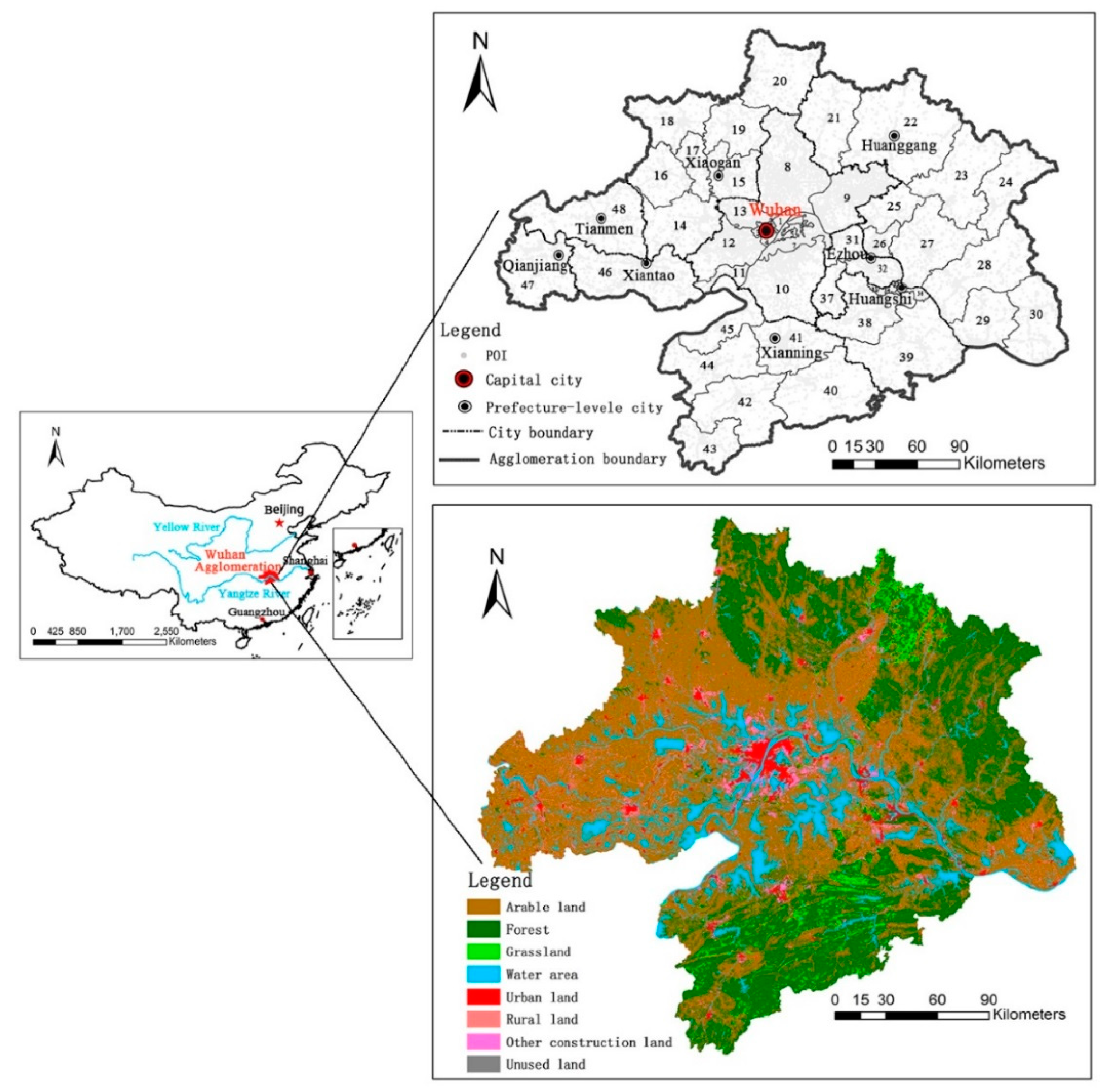
The Wuhan urban agglomeration is situated in the eastern part of Hubei Province (upper left longitude 112°30′ E and latitude 29°05′ N, lower right longitude 116°10′ E and latitude 31°50′ N) [27]. The Wuhan urban agglomeration includes the capital of Hubei Province (i.e., Wuhan) and eight other prefecture-level cities, namely, Huangshi, Ezhou, Xiaogan, Xianning, Xiantao, Huanggang, Qianjiang, and Tianmen (Figure 1). This agglomeration is composed of 48 counties and covers a total area of approximately 58,000 km2, which is less than one-third the size of Hubei Province [28]. Nevertheless, the Wuhan urban agglomeration accounts for more than 50% of the population and gross domestic product (GDP) of Hubei Province [29]. The Wuhan urban agglomeration includes Jianghan Plain, and the Yangtze River runs from west to east. The water area is 6344 km2, accounting for 11% of the total area in 2015 according to Landsat TM images. The Wuhan urban agglomeration was selected in this study because it is one of the largest and fastest growing urban agglomerations in China with a strategic position [28]. Similar to its central city, namely, Wuhan, the theme of which is “Wuhan, Different Every Day”, the Wuhan urban agglomeration is highly representative of urbanization [27].
The data used included interpreted land use maps from Landsat TM images in 2010 and 2015, with a spatial resolution of 30 m. Thematic land use maps (Figure 1) with eight categories, namely, arable land, forest, grassland, water area, urban area, rural area, other construction land, and unused land, were generated on the basis of the National Land Use Classification System (GB/T21010-2007) and the image processing results. The point of interest (POI) map of China was provided by Baidu open platform (http://lbsyun.baidu.com/index.php?title=lbscloud/poitags), and the POI for the Wuhan urban agglomeration was extracted (Figure 1). The income, population, GDP, revenue, agricultural output, consumption, and fixed asset investment of all the counties were collected from the Wuhan City Yearbook (2010–2016), Hubei Yearbook (2010–2016), and Chinese City Yearbook (2010–2016). Not all the indices were available for the 48 counties in the agglomeration area. Thus, regressions and predictions were used as substitutes for the missing data.
2.2. Methods
2.2.1. Calculation of ECC
ECC can be calculated using various methods, with the ecological footprint being the most widely applied one [30,31]. The ecological footprint analysis method proposed by Rees and Wachernagel in 1992 is used to calculate ECC according to biological physical quantity. This method balances the imperfections of single carrying capacity models for resources or the environment and helps obtain necessary data [32]. Owing to its straightforwardness and effectiveness, this method has been employed by many scholars worldwide to evaluate ecological environmental quality and sustainable development [32,33,34,35,36]. Furthermore, most studies transformed the calculation of ECC into measurements of ecologically productive land areas through the quantification of a set of indicators [37,38], which have been widely used to assess ECC at different levels [39,40]. Specifically, the calculation equation for ECC is as follows:
where ECC is the total ECC, N represents the population, ecc is the per capita ECC, 12% represents 12% of the land area deducted from the total area since the beginning of biodiversity conservation, j is the type of land use, aj is the ecological productive land area per capita, rj is the equilibrium factor, and yj is the yield factor. The data of the equilibrium factors were based on the “Living Planet Report” published by the World Wildlife Fund [41], and the data of the yield factors were adjusted on the basis of the output level in the study area [42] (Table 1).
2.2.2. Calculation of Land Urbanization Rate
Urban development leads to urban land expansion, sprawl, and regeneration, thereby providing a basis for the formation of land urbanization. The boundary of an urbanized land area is defined as the urban spatial extent that has actually been constructed and developed. It has the essential urban infrastructure and facilities to meet the needs of daily life and production activities of residents. Several studies used data from arbitrarily delineated areas obtained by the government, land surveying, or land use classification from remote sensing to represent urban land areas for calculating land urbanization [43]. However, this approach may induce bias or limitation because urbanized land is neither defined by the government nor confined to its superficial or spectral attributes. It is closely related to human activities and the physical attachments on the land. In the intersection of urban and rural areas, suburban areas, or urban fringes, the socio-economic development is high level. Moreover, anthropogenic activities are closely linked to the city. In this sense, these intersection area should also be regarded as part of the urbanized area. The urban–rural boundary threshold is a key element in determining the boundary of urban built-up areas, whereas the threshold in the existing literature often depends on human judgment [44,45].
In fact, a new method that identifies the boundaries of urbanized areas on the basis of the kernel density distribution of the POI data has become popular [24,25]. POI data refer to points, polylines, or polygons that describe the spatial distribution of primary infrastructure and facilities, such as shopping centers, hospitals, schools, and restaurants. POIs have various classifications according to regional characteristics and research objectives [46]. We classified POI data by considering the POIs that are used to derive urbanized land as follows (Table 2).
Kernel density and the densi-graph method are combined to obtain the boundary of the urbanized area. Kernel density estimation enables high-quality density estimation of point data without being affected by grid size and grid position [47], and it has been widely used in spatial analysis, especially in identifying urban–rural fringes [48,49]. The spatial distribution differences of POI density reflect the varying regional development levels, and the density in urbanized areas is generally higher than that in rural areas. Specifically, the estimated density of each point is the weighted average density of all points in the area. The kernel density Pi of an arbitrary point i in space is defined as the highest density and exhibits an outward decreasing function at the center (2):
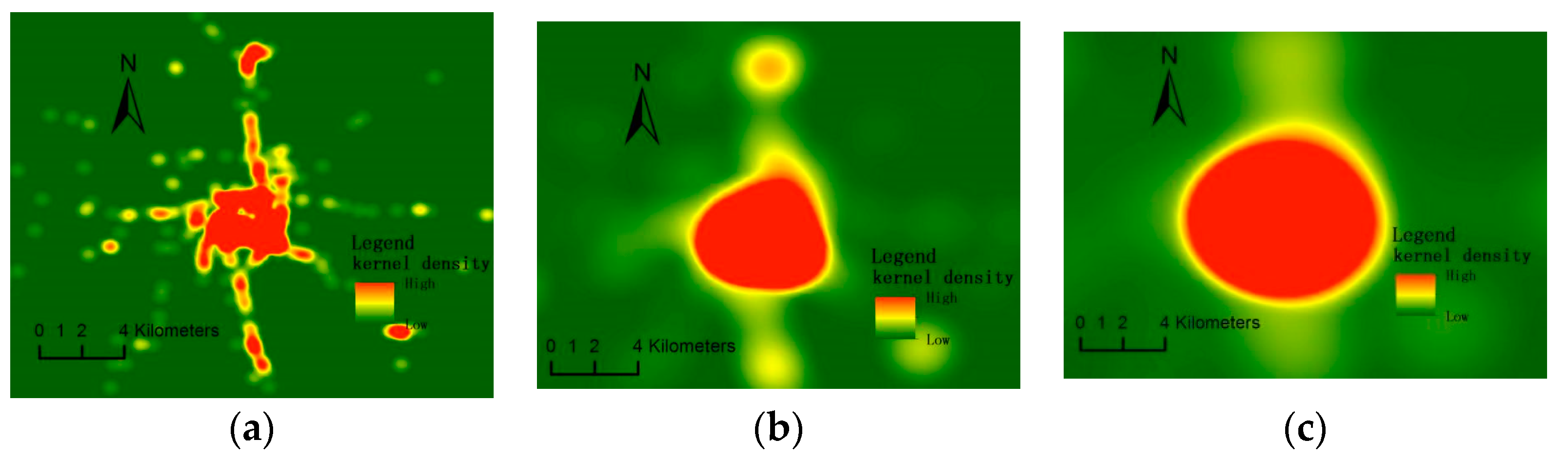
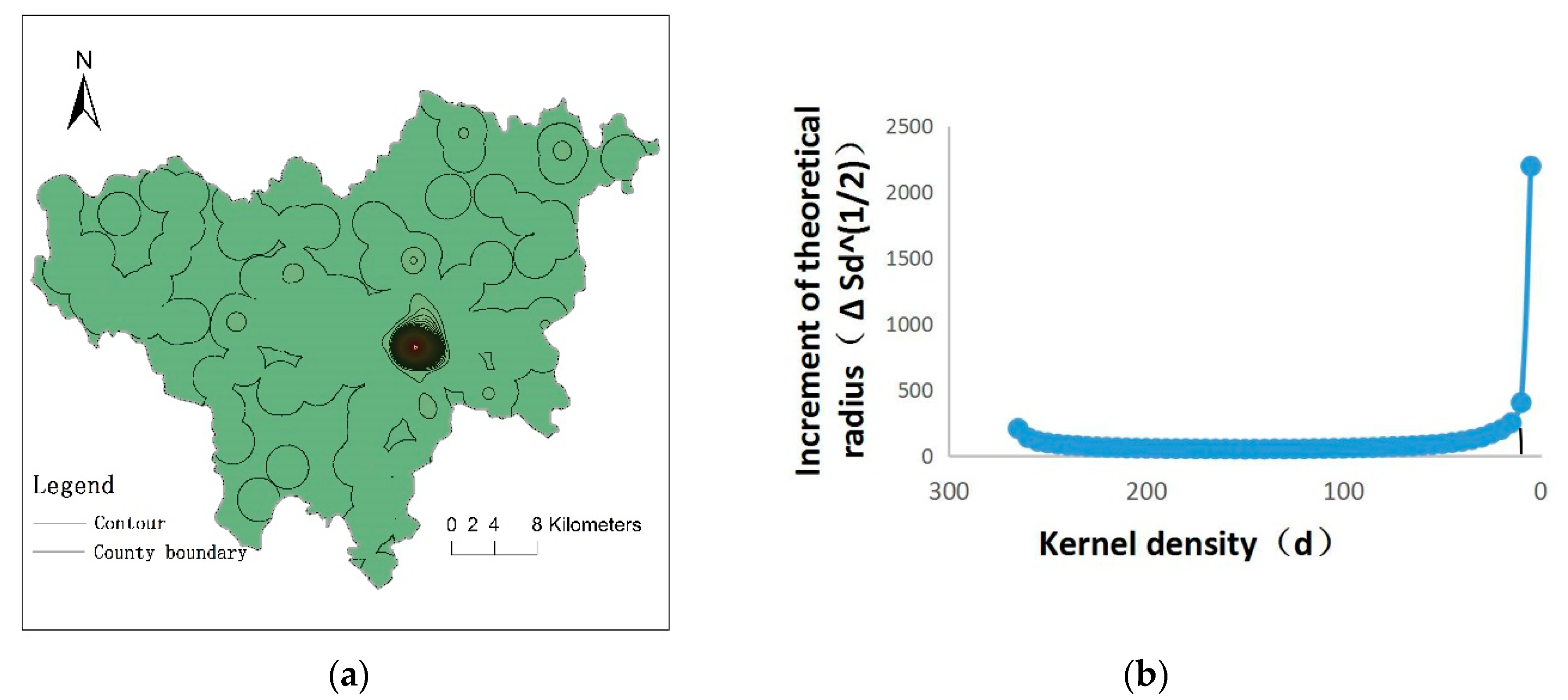
where Kj is the weight of the target j, Dij is the distance between neighboring point i and target j, R is the bandwidth of the selected regular region (Dij < R), and n is the range of the bandwidth R within the quantity of study object j. The selection of bandwidth R exerts a remarkable effect on the results of kernel density analysis [50], and a certain amount of bandwidth keeps the density center stable [51]. R is 2000 in 2015 and 1000 in 2010 according to the estimation of POI density distribution in different years (Figure 2). Then, the densi-graph method is proposed to identify the actual urbanized areas using the contour map of the kernel density of the POI [25].The basic idea of the densi-graph is to obtain the urbanized area through the discovery of the point with abrupt change through the contour map generated by the kernel density estimation of POIs. In the first step, we produced the contour lines with consecutively increasing radii according to the kernel density estimation of POIs in each county. Then, we calculated the closed areas Sd and the corresponding theoretical radius at each density point in each county. Subsequently, we produced the densi-graph with the density value d as the x-axis and the theoretical radius increment as the y-axis. Finally, we induced the critical point in the densi-graph, which showed the density curve undergoing an abrupt increase through differentiation and normalization; this curve was regarded as the threshold to generate the boundary of the urbanized and non-urbanized areas. We used the urbanized land percentage (ULP) to represent land urbanization (3).
where ULPi is the urbanized area in the ith county, ULi represents the urban land area of the ith county, and Si represents the land area of the ith county.
2.2.3. Driving Factors and Spatial Interactions in Land Urbanization
The most widely accepted driving factors of land urbanization, urban sprawl, and urban land expansion can be categorized into socioeconomic, proximity, physical, accessibility, and neighborhood aspects on the basis of the review of existing studies [52]. By considering empirical studies, regional characteristics, and data accessibility, we selected nine potential factors, namely, disposable personal income for rural residents (DPIR), disposable personal income for urban residents (DPIU), proportion of contribution of second industries to GDP (PSI), proportion of contribution of tertiary industries to GDP (PTI), fixed asset investment per area (PFAI), government revenue per area (PGV), agricultural output value per capita (PAU), foreign trade export per area (PFT), and retail sales of consumer goods per capita (PRSC) [53,54,55]. We used “per capita” or “per area” to transform these explanatory variables into ratio form for comparison. Then, we performed correlation and regression analyses to find highly correlated factors and eliminate multicollinearity.
Spatial dependence and influence, which reflect the necessity to incorporate spatial effects into operational models, are widely considered in statistical calculation and regional science [56]. Spatial regression has been proven to be a suitable method for spatially identifying the urban expansion mechanism [57]. This approach provides a theoretical basis and spatial analysis technique for exploring underlying driving forces. In our study, the spatial interactions among ecological counties were represented by the mutual transfer process of urban ECC [58]. The spatial interactions among counties decline due to the distance among them, as described by Newton’s law of universal gravitation. The gravity between two ecological counties can be described as follows Equation (4):
where Eij is the ecological gravity between ecological counties i and j, ki and kj represent the ECC per capita that the two ecological counties can provide, dij is the distance between the two ecological counties, and r is the constant for the interaction of the ecological counties and is r = 1 in this study [58].
Spatial autocorrelation analysis is also performed to test whether the observations of a variable with a spatial position are closely associated with the observations at adjacent spatial points. Moran’s I is a commonly used indicator that can be divided into two local spatial autocorrelation aspects [59]. We used global spatial autocorrelation to measure the degree of urban decentralization, which is defined as Equation (5):
where n represents the number of observations, which is 48 in the Wuhan urban agglomeration; xi is the value of ULP in the ith county; xj is the value of ULP for county yj; is the mean value; and wij is the value of the spatial weight matrix [60].
3. Results
3.1. ECC in the Wuhan Urban Agglomeration
Table 3 presents the ECC per capita of the counties in the Wuhan urban agglomeration in 2010 and 2015. The largest ECC per capita was observed in Liangzihu District, which is located in the south of the city circle (5.6166 hm2/cap in 2010 and 5.5393 hm2/cap in 2015), whereas the smallest ECC was observed at the center of the city circle, that is, Jianghan District (0.0589 hm2/cap in 2010 and 0.0389 hm2/cap in 2015). From 2010 to 2015, 13 counties exhibited an increase in ECC per capita, and the maximum increase of 0.9739 hm2/cap occurred in Caidian District. A total of 35 counties demonstrated a decrease in ECC per capita, and the maximum decrease of 2.7199 hm2/cap occurred in Qinshui County. The unit of improving ECC in the urban circle was less than the unit of declining ECC in the Wuhan urban agglomeration, and the average ECC per capita decreased.
3.2. Land Urbanization in the Wuhan Urban Agglomeration
Figure 2 illustrates the kernel estimation of bandwidths with 500, 2000, and 4000 m in 2015. The kernel density distribution is too scattered in the 500 m bandwidth and is too aggregated in the 4000 m bandwidth. As a result, we selected 2000 m as the appropriate bandwidth to estimate the kernel density and produce a contour line map, as presented in Figure 3a. The densi-graph curve was generated (Figure 3b) to identify the point of abrupt change. Using the combined kernel density estimation and the densi-graph method in the 48 counties in the Wuhan urban agglomeration, we determined that the captured differentiated and normalized radius values with abrupt changes were 20% in 2010 and 5% in 2015. Twelve counties had a threshold of 2% in 2010, and nine counties had a threshold value of 5‰ in 2015.
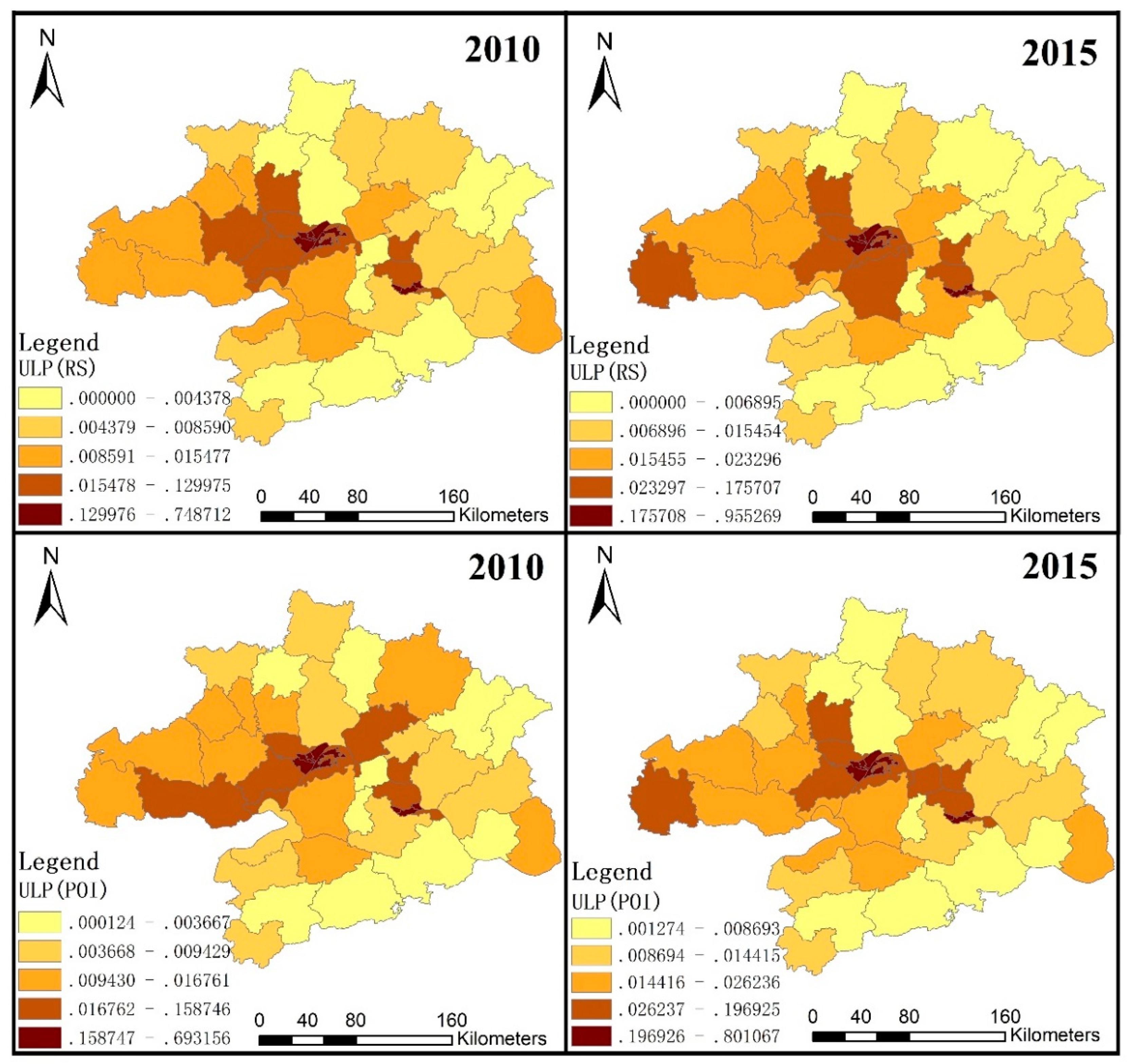
We also compared the results of the urbanized land area extracted using the densi-graph method and the urban land area obtained from remote sensing images. Figure 4 further illustrates the results of urban land extraction through remote sensing images and the results of urbanized land area obtained through the combined kernel density and densi-graph method. The urbanized land area is slightly higher than the urban area because we included suburban areas or urban fringes with considerable urban infrastructure and great development potential. In this sense, the measurement of land urbanization is accurate given the focus on the “real” construction and terrestrial attributes of urbanized land. In terms of ULP, 45 counties exhibited an evident increase from 2010 to 2015, and the highest increment (24.64%) was recorded in Jiangan District. The land urbanization degrees in Qingshan District, Tieshan District, and Xisaishan District declined, but the decrease was less than 10%. The highest ULP values were observed in the central and western areas, particularly in the urban district of Wuhan. By contrast, the counties in the south, southeastern, and northeastern areas presented the least urbanization values.
3.3. Driving Forces and Spatial Effects of ECC on Land Urbanization
3.3.1. Driving Forces of Land Urbanization Change
Table 4 lists the important variables for urbanization in 2010 and 2015. As shown in the table, certain factors, such as PTI, PFAI, DPIU, DPIR, PGV, PAU, PFT, and PRSC, considerably influenced land urbanization in 2010 and 2015. PFAI and PGV were the most highly correlated indicators in 2010 and 2015.
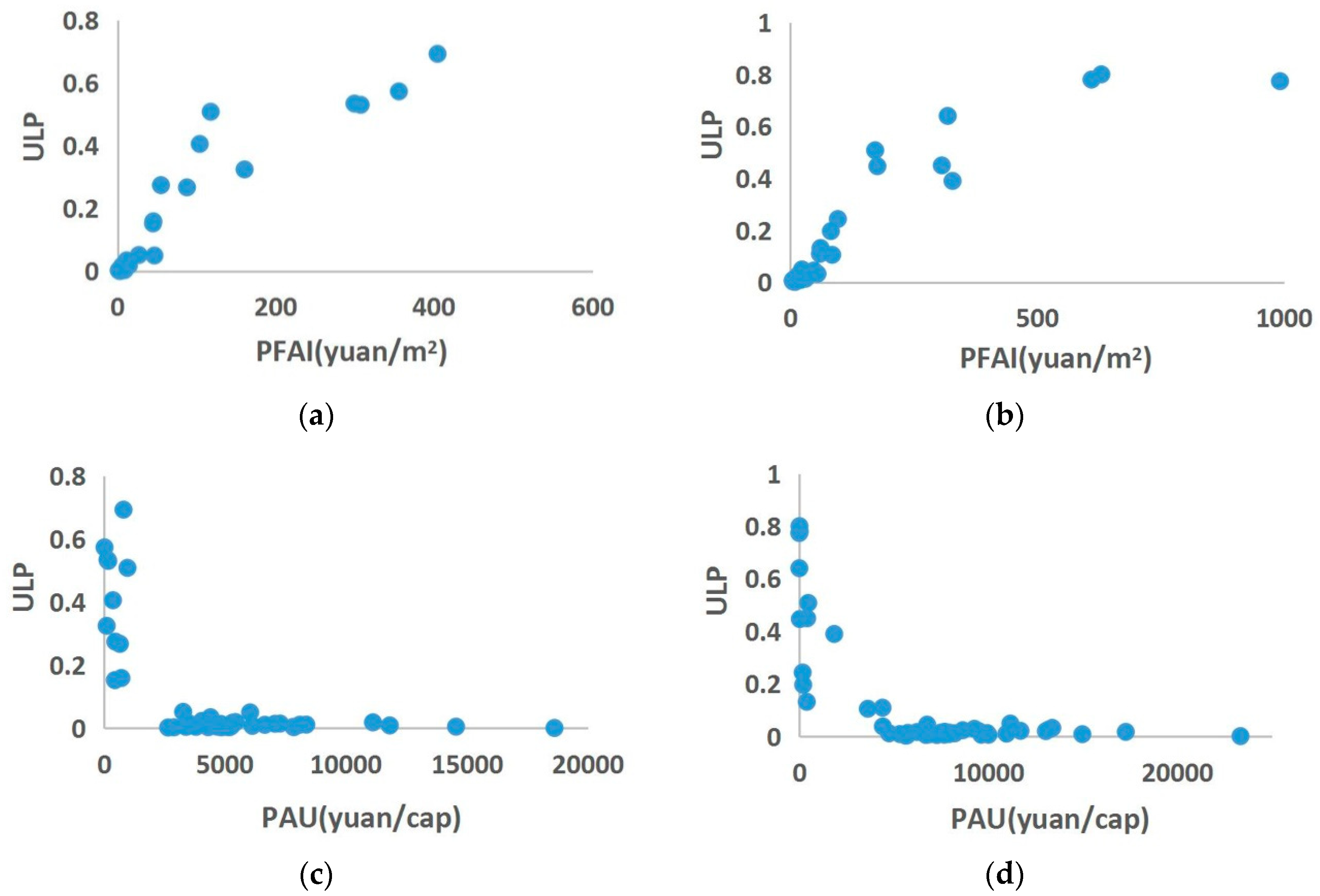
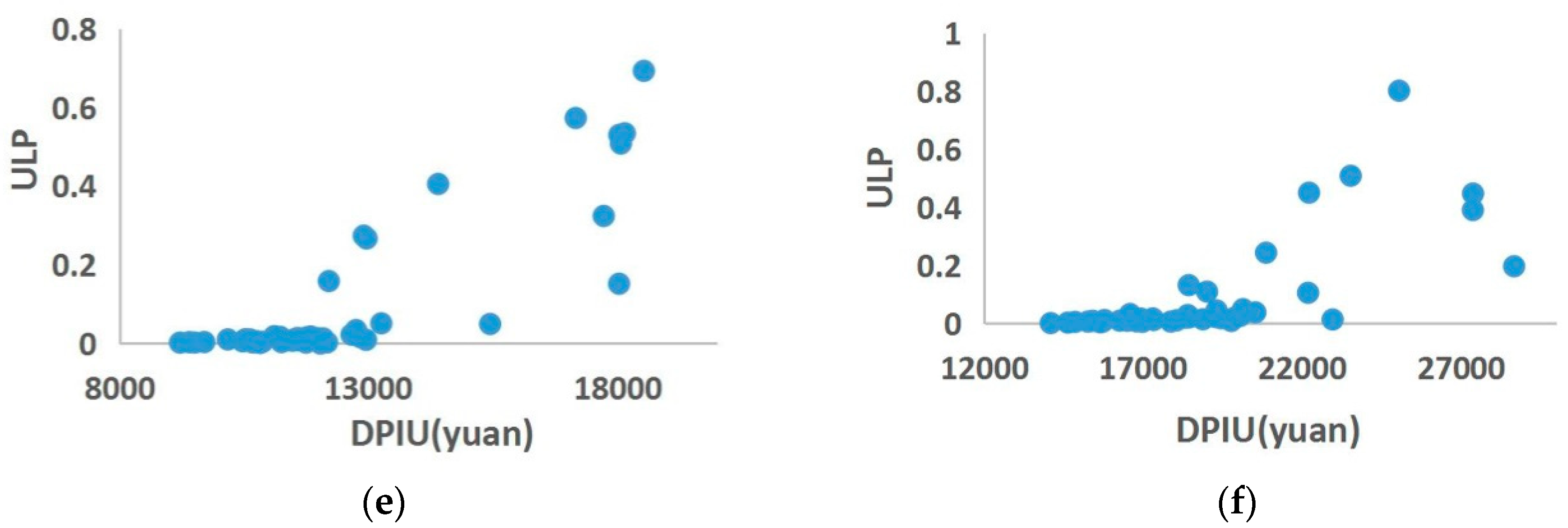
After performing a regression analysis using different combinations of the significant variables in 2010 and 2015, we finally selected fixed asset investment (PFAIi (yuan/m2)), agricultural output (PAUi (yuan/cap)), and income (DPIU (yuan/m2)) as the potential driving factors of land urbanization. These three factors were calculated as the ratio of fixed asset investment to the total land area, the ratio of agricultural output to the total population, and the per capita income of urban residents. The scatterplots of PFAI, PAU, and DPIU with land urbanization in 2010 and 2015 are illustrated in Figure 5a–f. PFAI and DPIU exerted a positive influence on land urbanization in 2010 and 2015, indicating that when PFAI and DPIU increased, land urbanization positively increased. In contrast, PAU exerted a negative effect on land urbanization in 2010 and 2015.
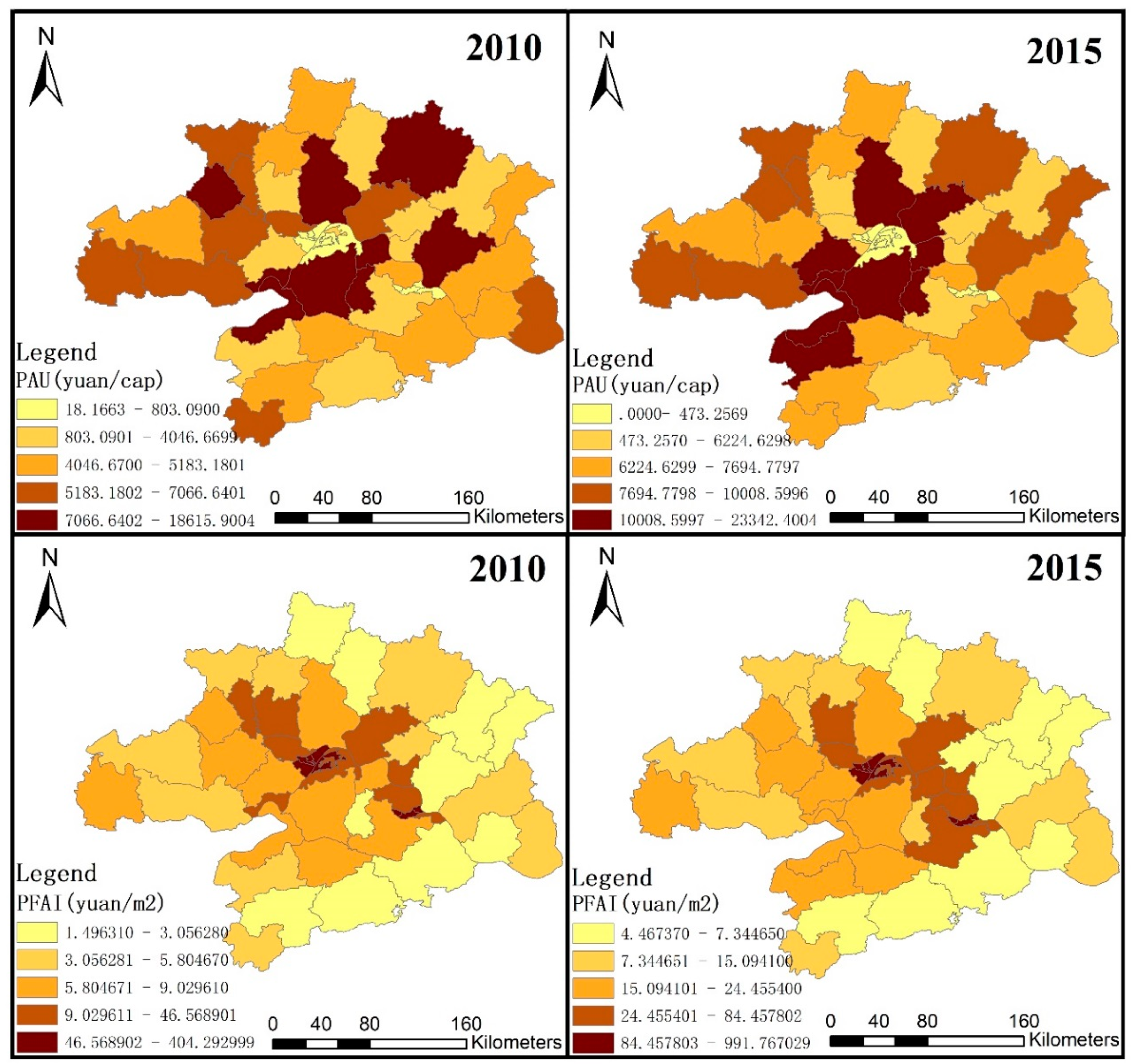
Figure 6 also illustrates the spatial patterns of PAU and PFAI in the Wuhan urban agglomeration in 2010 and 2015. The values of PAU and PFAI increased from 2010 to 2015, particularly in the central area of the Wuhan urban agglomeration. Moreover, counties around Wuhan had higher government revenues and fixed asset investments than other counties. In contrast, the urban district in Wuhan had the lowest agricultural output.
3.3.2. Spatial Effects of ECC on Land Urbanization
Table 5 presents the spatial interaction of ecological carrying capacities per capita amongst counties calculated through gravity model in the Wuhan urban agglomeration in 2010 and 2015. The strongest spatial interaction was observed between Caidian Disrtict and Hannan District, which are suburban districts of Wuhan city (2.9191 m2/cap2 in 2010 and 3.6507 m2/cap2 in 2015). From 2010 to 2015, the average gravity value of spatial interaction of ecological carrying capacities per capita amongst counties decreased.
A spatial autocorrelation was identified, and the values of Moran’s I for ULP were 0.3250 and 0.3222 in 2010 and 2015, respectively. Table 6 summarizes the spatial regression results in 2010 and 2015. A spatial relation was observed in the land urbanization process because the spatial coefficients in 2010 and 2015 were significant. The spatial interactions among counties at different ECCs per capita were high in 2010 and 2015. The spatial regression results provide a high degree of explanation given that R2 is higher than 0.9.
4. Discussion
Land urbanization is a spatio-temporal process that involves capital investment, infrastructure construction, social and government support, and ecological adjustment [61,62,63]. During this process, urban land expansion is inevitable, and ECC is proved to be an effective way to prevent eco-environmental problems and balance the socio-economic development and sustainable ecosystems [20,64]. At the regional level, the contribution of these factors to the expanded urbanized land and the effects of the spatial interactions generated from eco-constraints on this process are of vital importance for the comprehension and optimization of sustainable land urbanization [65,66].
The primary contributions of our study lie in two aspects, namely, the exploration of the spatial effects of ECC on land urbanization and the quantification of land urbanization using the densi-graph method. On the one hand, land urbanization has been closely related to urban expansion and is also generally accompanied by a decrease in ecological land [67,68,69]. In China, the proportion of ecological land space decreased by 0.85%, whereas the proportion of urban land space increased by 1.53% from 1984 to 2012 [17]. A high proportion of ecological land predictably yields high ecological footprint and ECC [70]. Therefore, the implicit and crucial relationship between ECC and land urbanization is plausible. However, previous studies primarily focused on the effects of land use change on ECC or the constraints and policy implications of ECC for the optimization of land use locally [20,71]. Spatial interaction, that is, the influences of ECC in one spatial unit on its neighboring spatial units, have seldom been explored in the context of ongoing land urbanization. In the contemporary socio-economic strategy, regional development has been underlined, and the evolution of the eco-environment has demonstrated increased regional characteristics [72,73]. Therefore, we used a gravity model to quantify the spatial interactions generated by ECC and embedded it into the spatial regression model to explore the importance and magnitude of this spatial influence in the Wuhan agglomeration. The average ECC per capita decreased, whereas the spatial interactions among the counties were substantial and exhibited a slight decline in 2010−2015. The results confirm that the spatial influence of ECC is a factor that cannot be neglected in promoting land urbanization. In fact, ECC reflects the ability of accommodating life and human production in one region, and the spatial influence among counties embodies resource allocation, transfer, compensation, and optimization [74]. Counties with high gravity induced by ECC are inclined to achieve a high degree of effective allocation and sustainable use of resources through various and vibrant trade-offs, which help coordinate regional development to achieve sustainable land urbanization [75]. Meanwhile, the quantification of urbanized land is essential in our study. We applied the densi-graph method based on POIs to obtain the urbanized land area. The reason behind this choice is that urban infrastructure on urbanized land should be sufficient and that the spatial distribution of these POIs should conform to certain density patterns [76]. We also compared the urbanized land area extracted through the densi-graph method and the urban area extracted from remote sensing images. The comparison showed that the urbanized land area is slightly higher than the urban area because we included suburban areas or urban fringes with considerable urban infrastructure and great development potential. In this sense, the measurement of land urbanization is accurate given the focus on the “real” construction and terrestrial attributes of urbanized land.
PFAI, PAU, and DPIU were found to be correlated with land urbanization, with PFAI being the most powerful. In general, the government tends to make investments in regions with favorable economic environment to enhance urban infrastructure and consequently accelerate the rapid expansion of urban built-up areas [77]. In addition, improved disposable personal income and consumption are also supposed to urge the government to expand urban land areas for commercial use, public facilities, and residence [78]. An increasing number of rural residents are also supposed to migrate to urban areas for job opportunities instead of engaging in agricultural activities [79]. Thus, a negative relationship between agricultural output and urbanization rate was observed. The use of strategic opportunities is advisable to achieve a new type of urbanization in which agricultural development, social opportunities, and economic investment are the key factors.
5. Conclusions
This study explored the spatial influence of ECC on land urbanization and the underlying driving forces using the Wuhan urban agglomeration as a case example. We devised spatial models with ECC-based spatial weight matrices for examining the potential spatial interactions or constraints and the influencing factors of land urbanization. Specifically, the densi-graph method based on the kernel density of POIs was used to derive the “real urban land,” and the ecological footprint analysis method was applied to calculate ECC. The results revealed the following; (1) Land urbanization in most counties increased, whereas the average ECC per capita decreased in the Wuhan urban agglomeration; (2) Fixed asset investment and urban income exerted positive influences on land urbanization, whereas agricultural output was negatively correlated with land urbanization; (3) Spatial interaction was formulated through ECC during the land urbanization process; however, this effect was attenuated slightly in 2010−2015.
In fact, spatially explicit models are preferable in exploring spatial interactions at the regional level, especially in the context of spatio-temporal processes such as land urbanization. However, spatial influences are not confined to ECC; other social, economic, political, and technological factors, such as social network and transportation, can also been considered as potential candidates to gauge spatial effects on land urbanization. In addition, we applied the POI-based densi-graph method to identify urbanized land at the county level. This approach improved accuracy to a certain extent. However, we applied fixed thresholds, which are incapable of capturing the local differences in different counties, when kernel density was analyzed. Thus, the adjusted threshold is also a potential tool to improve our method. In the future, other integrated, dynamic, and spatially heterogeneous methods for exploring the driving mechanisms of land urbanization should be proposed to achieve sustainable urban development.
Author Contributions
Conceptualization, C.Z.; Data curation, Y.L. and H.C.; Funding acquisition, C.Z.; Investigation, Y.L.; Methodology, Y.S.; Project administration, C.Z.; Resources, H.C.; Software, Y.S.; Writing—original draft, Y.L.
Funding
the Natural Science Foundation of China (41771563, 41501179) funded this research and the APC was funded by the Innovation Fund from Huazhong Agricultural University (2662018PY094).
Acknowledgments
The author is grateful to the members of the Chinese Cities Research Center, Department of City and Regional Planning, University of North Carolina-Chapel Hill for their valuable advice.
Conflicts of Interest
The authors declare no conflicts of interest.
References
- Wang, X.R.; Hui, C.M.; Choguill, C.; Jia, S.H. The new urbanization policy in China: Which way forward? Habitat Int. 2015, 47, 279–284. [Google Scholar] [CrossRef]
- United Nations (UN). World Urbanization Prospects: The 2018 Revision: Highlights; United Nations: New York, NY, USA, 2018. [Google Scholar]
- Liu, J.; Zhan, J.; Deng, X. Spatio-temporal patterns and driving forces of urban land expansion in China during the economic reform era. Ambio 2005, 34, 450–455. [Google Scholar] [CrossRef] [PubMed]
- Chen, M.; Liu, W.; Lu, D. Challenges and the way forward in China’s new-type urbanization. Land Use Policy 2016, 55, 334–339. [Google Scholar] [CrossRef] [Green Version]
- Maruotti, A. The impact of urbanization on CO2 emissions: Evidence from developing countries. Ecol. Econ. 2011, 70, 1344–1353. [Google Scholar]
- Zhang, X.; Chen, J.; Tan, M.; Sun, Y. Assessing the impact of urban sprawl on soil resources of Nanjing city using satellite images and digital soil databases. Catena 2007, 69, 16–30. [Google Scholar] [CrossRef]
- Chen, J. Rapid urbanization in China: A real challenge to soil protection and food security. Catena 2007, 69, 1–15. [Google Scholar] [CrossRef]
- United Nations. Transforming Our World: The 2030 Agenda for Sustainable Development; United Nations: New York, NY, USA, 2015. [Google Scholar]
- Rees, W.E. Revisiting carrying capacity: Area-based indicators of sustainability. Popul. Environ. 1996, 17, 195–215. [Google Scholar] [CrossRef]
- Prato, T. Fuzzy adaptive management of social and ecological carrying capacities for protected areas. J. Environ. Manag. 2009, 90, 2551–2557. [Google Scholar] [CrossRef] [PubMed]
- Abernethy, V.D. Carrying capacity: The tradition and policy implications of limits. Ethics Sci. Environ. Polit. 2001, 2001, 9–18. [Google Scholar] [CrossRef]
- Zeng, C.; Liu, Y.F.; Zhang, W.S.; Tang, D.W. Origination and development of the concept of aquatic ecological carrying capacity in the basin. Resour. Environ. Yangtze Basin 2011, 20, 203–210. [Google Scholar]
- Dong, L.; Feng, Z.; Yang, Y.; Zhen, Y. Spatial patterns of ecological carrying capacity supply-demand balance in China at county level. J. Geogr. Sci. 2011, 21, 833–844. [Google Scholar]
- Zhang, M.; Liu, Y.; Wu, J.; Wang, T. Index system of urban resource and environment carrying capacity based on ecological civilization. Environ. Impact Assess. Rev. 2018, 68, 90–97. [Google Scholar] [CrossRef]
- Fang, W.; An, H.; Li, H.; Gao, X.; Sun, X. Urban economy development and ecological carrying capacity: Taking Beijing city as the case. Energy Procedia 2017, 105, 3493–3498. [Google Scholar] [CrossRef]
- Attwell, K. Urban land resources and urban planting—Case studies from Denmark. Landsc. Urban Plan. 2000, 52, 145–163. [Google Scholar] [CrossRef]
- Wang, J.; He, T.; Lin, Y. Changes in ecological, agricultural, and urban land space in 1984–2012 in China: Land policies and regional social-economical drivers. Habitat Int. 2018, 71, 1–13. [Google Scholar] [CrossRef]
- Li, A.; Kang, R.; Yang, H. Construction and analysis of rapid urbanization regional ecological carrying capacity evaluation model. Environ. Sci. Manag. 2013, 2, 139–143, 164. [Google Scholar]
- Zhang, Y.; Yang, Q.; Min, J. An analysis of coupling between the bearing capacity of the ecological environment and the quality of new urbanization in Chongqing. Acta Geogr. Sin. 2016, 71, 817–828. [Google Scholar]
- Peng, J.; Du, Y.; Liu, Y.; Hu, X. How to assess urban development potential in mountain areas? An approach of ecological carrying capacity in the view of coupled human and natural systems. Ecol. Indic. 2016, 60, 1017–1030. [Google Scholar] [CrossRef]
- Cao, Z.; Min, Q.W.; Liu, M.C.; Bai, Y.Y. Ecosystem-service-based ecological carrying capacity: Concept, content, assessment model and application. J. Nat. Resour. 2015, 30, 1–11. [Google Scholar]
- Liu, Z.; He, C.; Zhang, Q.; Huang, Q.; Yang, Y. Extracting the dynamics of urban expansion in China using DMSP-OLS nighttime light data from 1992 to 2008. Landsc. Urban Plan. 2012, 106, 62–72. [Google Scholar] [CrossRef]
- Jing, W.; Yang, Y.; Yue, X.; Zhao, X. Mapping urban areas with integration of DMSP/OLS nighttime light and MODIS data using machine learning techniques. Remote Sens. 2015, 7, 12419–12439. [Google Scholar] [CrossRef]
- Duan, Y.M.; Liu, Y.; Liu, X.H.; Wang, H.L. Identification of polycentric urban structure of central Chongqing using points of interest big data. J. Nat. Resour. 2018, 33, 788–800. [Google Scholar]
- Zening, X.U.; Gao, X. A novel method for identifying the boundary of urban built-up areas with poi data. Acta Geogr. Sin. 2016, 71, 928–939. [Google Scholar]
- Qin, R.; Li, J.; Tang, H. A Method for Extracting Urban Built-Up Area Based on RS Indexes; Society of Photo-Optical Instrumentation Engineers (SPIE) Conference Series; Society of Photo-Optical Instrumentation Engineers: Bellingham, WA, USA, 2016; Volume 10156, p. 101561V. [Google Scholar]
- Zhang, L.; Zhang, M.; Yao, Y. Mapping seasonal impervious surface dynamics in Wuhan urban agglomeration, China from 2000 to 2016. Int. J. Appl. Earth Obs. Geoinf. 2018, 70, 51–61. [Google Scholar] [CrossRef]
- Tan, R.; Liu, Y.; Liu, Y.; He, Q.; Ming, L.; Tang, S. Urban growth and its determinants across the Wuhan urban agglomeration, central China. Habitat Int. 2014, 44, 268–281. [Google Scholar] [CrossRef]
- Chen, Z.; Zhang, A.; Shan, X. Urbanization and administrative restructuring: A case study on the Wuhan urban agglomeration. Habitat Int. 2016, 55, 46–57. [Google Scholar] [Green Version]
- Liu, N.F.; Yao, R.Z.; Liu, R.; Song, W.W. Ecological carrying capacity and tourism sustainability based on ecological footprint analysis. Environ. Sci. Technol. 2005, 28, 95–97. [Google Scholar]
- Xie, F.; Zheng, M.; Hong, Z. Research on ecological environmental carrying capacity in Yellow River Delta. Energy Procedia 2011, 5, 1784–1790. [Google Scholar]
- Miao, C.L.; Sun, L.Y.; Yang, L. The studies of ecological environmental quality assessment in Anhui province based on ecological footprint. Ecol. Indic. 2016, 60, 879–883. [Google Scholar] [CrossRef]
- Hopton, M.E.; White, D. A simplified ecological footprint at a regional scale. J. Environ. Manag. 2012, 111, 279. [Google Scholar] [CrossRef] [PubMed]
- Butnariu, A.; Avasilcai, S. Research on the possibility to apply ecological footprint as environmental performance indicator for the textile industry. Procedia Soc. Behav. Sci. 2014, 124, 344–350. [Google Scholar] [CrossRef]
- Galli, A. On the rationale and policy usefulness of ecological footprint accounting: The case of morocco. Environ. Sci. Policy 2015, 48, 210–224. [Google Scholar] [CrossRef]
- Galli, A.; Kitzes, J.; Niccolucci, V.; Wackernagel, M.; Wada, Y.; Marchettini, N. Assessing the global environmental consequences of economic growth through the ecological footprint: A focus on China and India. Ecol. Indic. 2012, 17, 99–107. [Google Scholar] [CrossRef]
- Xin-Bo, D.U.; Qin, J. A case study on Haixi County, Qinghai Province: Regional eco-environmental load assessment based on ecological footprint. Resour. Ind. 2010, 12, 56–60. [Google Scholar]
- Wang, S.; Yang, F.L.; Xu, L.; Du, J. Multi-scale analysis of the water resources carrying capacity of the Liaohe basin based on ecological footprints. J. Clean. Prod. 2013, 53, 158–166. [Google Scholar] [CrossRef]
- Sun, L. Some problems and improvement measures of agricultural ecological environment in Wanbei. Anhui Agric. Sci. Bull. 2008, 12, 14–17, 83. [Google Scholar]
- Lei, B.; Zhou, X.; Ya-Kun, W.U.; Zhang, L. Assessment and strategies of eco-environment quality in downtown areas of Chongqing. Environ. Sci. Technol. 2012, 35, 200–205. [Google Scholar]
- World Wide Fund for Nature (WWF). Living Planent Report 2014; WWF: Gland, Switzerland, 2014. [Google Scholar]
- Yang, L.D.; Zeng, C.; Jiao, L.M.; Liu, Y. Evaluation on ecological carrying capacity and ecological compensation in Wuhan urban agglomeration based on ecological footprint. Resour. Environ. Yangtze Basin 2017, 26, 1332–1341. [Google Scholar]
- Yao, Y.; Chen, D.; Chen, L.; Wang, H.; Guan, Q. A time series of urban extent in China using DSMP/OLS nighttime light data. PLoS ONE 2018, 13, e0198189. [Google Scholar] [CrossRef] [PubMed]
- Imhoff, M.L.; Lawrence, W.T.; Stutzer, D.C.; Elvidge, C.D. A technique for using composite DMSP/OLS “city lights” satellite data to map urban area. Remote Sens. Environ. 1997, 61, 361–370. [Google Scholar] [CrossRef]
- Cheng, F.; Thiel, K.H. Delimiting the building heights in a city from the shadow in a panchromatic SPOT-image—Part 1. Test of forty-two buildings. Int. J. Remote Sens. 1995, 16, 409–415. [Google Scholar] [CrossRef]
- Zeng, C.; Yang, L.; Dong, J. Management of urban land expansion in China through intensity assessment: A big data perspective. J. Clean. Prod. 2016, 153, 637–647. [Google Scholar] [CrossRef]
- Dehnad, K. Density estimation for statistics and data analysis. Technometrics 1986, 29, 495. [Google Scholar] [CrossRef]
- Yu, W.; Ai, T.; Shao, S. The analysis and delimitation of central business district using network kernel density estimation. J. Transp. Geogr. 2015, 45, 32–47. [Google Scholar] [CrossRef]
- Peng, J.; Zhao, S.; Liu, Y.; Tian, L. Identifying the urban-rural fringe using wavelet transform and kernel density estimation: A case study in Beijing City, China. Environ. Model. Softw. 2016, 83, 286–302. [Google Scholar] [CrossRef]
- Heidenreich, N.B.; Schindler, A.; Sperlich, S. Bandwidth selection for kernel density estimation: A review of fully automatic selectors. AStA Adv. Stat. Anal. 2013, 97, 403–433. [Google Scholar] [CrossRef]
- Hinneburg, A.; Keim, D.A. An efficient approach to clustering in large multimedia databases with noise. In Proceedings of the International Conference on Knowledge Discovery and Data Mining, New York, NY, USA, 27–31 August 1998; Volume 98, pp. 58–65. [Google Scholar]
- Li, G.; Sun, S.; Fang, C. The varying driving forces of urban expansion in China: Insights from a spatial-temporal analysis. Landsc. Urban Plan. 2018, 174, 63–77. [Google Scholar] [CrossRef]
- Deng, X.; Huang, J.; Rozelle, S.; Uchida, E. Economic growth and the expansion of urban land in China. Urban Stud. 2010, 47, 813–843. [Google Scholar] [CrossRef]
- Liu, Y.; Yin, G.; Ma, L.J.C. Local state and administrative urbanization in post-reform China: A case study of Hebi City, Henan Province. Cities 2012, 29, 107–117. [Google Scholar] [CrossRef]
- Seto, K.C.; Güneralp, B.; Hutyra, L.R. Global forecasts of urban expansion to 2030 and direct impacts on biodiversity and carbon pools. Proc. Natl. Acad. Sci. USA 2012, 109, 16083–16088. [Google Scholar] [CrossRef] [PubMed] [Green Version]
- Zeng, C.; Zhang, A.; Liu, L.; Liu, Y. Administrative restructuring and land-use intensity—A spatial explicit perspective. Land Use Policy 2017, 67, 190–199. [Google Scholar] [CrossRef]
- Yu, D.; Wei, Y.D. Spatial data analysis of regional development in greater Beijing, China, in a GIS environment. Pap. Reg. Sci. 2008, 87, 97–117. [Google Scholar] [CrossRef]
- Wen, Z.C. Research on Development and Evaluation of Eco-City; Harbin Engineering University: Harbin, China, 2008. [Google Scholar]
- Torrens, P.M. A toolkit for measuring sprawl. Appl. Spat. Anal. Policy 2008, 1, 5–36. [Google Scholar] [CrossRef]
- LeSage, J.; Pace, R.K. Introduction to Spatial Econometrics; CRC Press: Boca Raton, FL, USA, 2008. [Google Scholar]
- Wu, Y.; Dong, S.; Huang, H.; Zhai, J.; Li, Y.; Huang, D. Quantifying urban land expansion dynamics through improved land management institution model: Application in Ningxia-Inner Mongolia, China. Land Use Policy 2018, 78, 386–396. [Google Scholar] [CrossRef]
- Zhang, Y.; Su, Z.; Li, G.; Zhuo, Y.; Xu, Z. Spatial-Temporal Evolution of Sustainable Urbanization Development: A Perspective of the Coupling Coordination Development Based on Population, Industry, and Built-Up Land Spatial Agglomeration. Sustainability 2018, 10, 1766. [Google Scholar] [CrossRef]
- Zhou, D.; Tian, Y.; Jiang, G. Spatio-temporal investigation of the interactive relationship between urbanization and ecosystem services: Case study of the Jingjinji urban agglomeration, China. Ecol. Indic. 2018, 95, 152–164. [Google Scholar] [CrossRef]
- He, C.; Han, Q.; de Vries, B.; Wang, X.; Guochao, Z. Evaluation of sustainable land management in urban area: A case study of Shanghai, China. Ecol. Indic. 2017, 80, 106–113. [Google Scholar] [CrossRef]
- Graymore, M.L.; Sipe, N.G.; Rickson, R.E. Regional sustainability: How useful are current tools of sustainability assessment at the regional scale? Ecol. Econ. 2008, 67, 362–372. [Google Scholar] [CrossRef]
- Chen, J.P.; Zeng, M.; Duan, Y.J. Regional carrying capacity evaluation and prediction based on GIS in the Yangtze River Delta, China. Int. J. Geogr. Inf. Sci. 2011, 25, 171–190. [Google Scholar] [CrossRef]
- Shu, B.; Zhang, H.; Li, Y.; Qu, Y.; Chen, L. Spatiotemporal variation analysis of driving forces of urban land spatial expansion using logistic regression: A case study of port towns in Taicang City, China. Habitat Int. 2014, 43, 181–190. [Google Scholar] [CrossRef]
- Li, C.; Li, J.; Wu, J. What drives urban growth in China? A multi-scale comparative analysis. Appl. Geogr. 2018, 98, 43–51. [Google Scholar] [CrossRef]
- Xia, C.; Li, Y.; Ye, Y.; Shi, Z. An integrated approach to explore the relationship among economic, construction land use, and ecology subsystems in Zhejiang Province, China. Sustainability 2016, 8, 498. [Google Scholar] [CrossRef]
- Yan-Mei, J.I. Dynamic change of land use and ecological carrying capacity in northern Shaanxi Province. China Popul. Resour. Environ. 2011, 21, 271–274. [Google Scholar]
- Qian, Y.; Tang, L.; Qiu, Q.; Xu, T.; Liao, J. A comparative analysis on assessment of land carrying capacity with ecological footprint analysis and index system method. PLoS ONE 2015, 10, e0130315. [Google Scholar] [CrossRef] [PubMed]
- Liu, X.; Huang, F. Analysis of the regional eco-environmental effect driving by LUCC. J. Northeast Norm. Univ. 2002, 34, 87–92. [Google Scholar]
- Liu, W.; Zhan, J.; Li, Z.; Jia, S.; Zhang, F.; Li, Y. Eco-efficiency evaluation of regional circular economy: A case study in Zengcheng, Guangzhou. Sustainability 2018, 10, 453. [Google Scholar] [CrossRef]
- Wang, S.F.; Xu, Y.; Liu, T.J.; Ye, J.M.; Pan, B.L.; Chu, C.; Peng, Z.L. Review of Evaluation on Ecological Carrying Capacity: The Progress and Trend of Methodology; IOP Conference Series: Earth and Environmental Science; IOP Publishing: Bristol, UK, 2018; Volume 113, p. 012108. [Google Scholar]
- Tian, Y.; Sun, C. A spatial differentiation study on comprehensive carrying capacity of the urban agglomeration in the Yangtze River Economic Belt. Reg. Sci. Urban Econ. 2018, 68, 11–22. [Google Scholar] [CrossRef]
- Ma, L.; Li, D.; Tao, X.; Dong, H.; He, B.; Ye, X. Inequality, Bi-Polarization and Mobility of Urban Infrastructure Investment in China’s Urban System. Sustainability 2017, 9, 1600. [Google Scholar] [CrossRef]
- Shu, C.; Xie, H.; Jiang, J.; Chen, Q. Is urban land development driven by economic development or fiscal revenue stimuli in China? Land Use Policy 2018, 77, 107–115. [Google Scholar] [CrossRef]
- Chen, J.; Gao, J.; Chen, W. Urban land expansion and the transitional mechanisms in Nanjing, China. Habitat Int. 2016, 53, 274–283. [Google Scholar] [CrossRef]
- Lin, Y.; Li, Y.; Ma, Z. Exploring the Interactive Development between Population Urbanization and Land Urbanization: Evidence from Chongqing, China (1998–2016). Sustainability 2018, 10, 1741. [Google Scholar] [CrossRef]
Figure 1.
Study area.

Figure 2.
Kernel estimation of different bandwidths in 2015. (a) Bandwidth = 500 m. (b) Bandwidth = 2000 m. (c) Bandwidth = 4000 m.
Figure 2.
Kernel estimation of different bandwidths in 2015. (a) Bandwidth = 500 m. (b) Bandwidth = 2000 m. (c) Bandwidth = 4000 m.

Figure 3.
Boundary of urban built-up area in a typical city in 2015. (a) Bandwidth = 2000 m. (b) Densi-Graph curve.
Figure 3.
Boundary of urban built-up area in a typical city in 2015. (a) Bandwidth = 2000 m. (b) Densi-Graph curve.

Figure 4.
Land urbanization in the Wuhan urban agglomeration in 2010 and 2015.

Figure 5.
Scatterplots of important factors for urbanization. (a) urbanized land percentage (ULP) and fixed asset investment per area (PFAI) in 2010. (b) ULP and PFAI in 2015. (c) ULP and agricultural output value per capita (PAU) in 2010. (d) ULP and PAU in 2015. (e) ULP and disposable personal income for urban residents (DPIU) in 2010. (f) ULP and DPIU in 2015.


Figure 6.
Representative factors in the Wuhan urban agglomeration in 2010 and 2015.


Table 1.
Description of land types.
| Land Type | Equilibrium Factor | Yield Factor |
|---|---|---|
| Arable land | 2.8 | 3.71 |
| Forest land | 1.1 | 0.91 |
| Grassland | 0.5 | 0.19 |
| Construction land | 2.8 | 3.71 |
| Water area | 0.2 | 176 |
| Energy land | 1.1 | 0 |
Table 2.
Point of Interest (POI) data type classification.
| ID | Main Category | Subdivided Category |
|---|---|---|
| 1 | Residential land | Residential |
| 2 | Land for administration and public services | Administrative agencies, schools, hospitals, and research institutes |
| 3 | Land for commercial and business facilities | Banks, restaurants, retail industries, commercial buildings, hotels, entertainment venues, and corporate enterprises |
| 4 | Industrial land | Factories |
| 5 | Transportation land | Transportation sites |
| 6 | Green space and square land | Parks, squares, and scenic spots |
Note: These data are based on the “Code for classification of urban land use and planning standards of development” (2011).
Table 3.
Description of ecological carrying capacity (ECC) (hm2/cap).
| Counties | Min | Max | Mean | Median | Variance | |
|---|---|---|---|---|---|---|
| 2010 | 48 | 0.0589 | 5.6166 | 1.8042 | 1.6659 | 1.5800 |
| 2015 | 48 | 0.0389 | 5.5393 | 1.7408 | 1.7299 | 1.4210 |
Table 4.
Important variables from the correlation analyses in 2010 and 2015.
| Variable | PSI | PTI | PFAI | PRSC | PGV | PFT | PAU | DPIU | DPIR |
|---|---|---|---|---|---|---|---|---|---|
| 2010 | −0.139 | 0.655 *** | 0.941 *** | 0.860 *** | 0.882 *** | 0.841 *** | −0.582 *** | 0.850 *** | 0.696 *** |
| 2015 | −0.368 ** | 0.734 *** | 0.915 *** | 0.831 *** | 0.849 *** | 0.738 *** | −0.652 *** | 0.835 *** | 0.617 *** |
Note: ** and *** indicate 5% and 1% significance levels, respectively.
Table 5.
Description of spatial interaction amongst counties (m2/cap2).
| Year | Counties | Min | Max | Mean | Median | Variance |
|---|---|---|---|---|---|---|
| 2010 | 48 | 0.0002 | 2.9191 | 0.0651 | 0.0183 | 0.0330 |
| 2015 | 48 | 0.0001 | 3.6507 | 0.0585 | 0.0165 | 0.0330 |
Table 6.
Spatial regression results in 2010 and 2015.
| Variable Scenario | OLS | Spatial Modeling | ||
|---|---|---|---|---|
| 2010 | 2015 | 2010 | 2015 | |
| PFAI | 0.001339 *** | 0.000753 *** | 0.001183 *** | 0.000671 *** |
| PAU | −0.000006 ** | −0.000007 ** | −0.000006 *** | −0.000007 *** |
| DPIU | 0.000016 *** | 0.000014 *** | 0.000013 ** | 0.000012 *** |
| Spatial coefficient | 0.581983 *** | 0.527995 ** | ||
| R2 | 0.919 | 0.9028 | 0.9157 | 0.9115 |
Note: ** and *** indicate 5% and 1% significance levels, respectively.
© 2018 by the authors. Licensee MDPI, Basel, Switzerland. This article is an open access article distributed under the terms and conditions of the Creative Commons Attribution (CC BY) license (http://creativecommons.org/licenses/by/4.0/).
Share and Cite
MDPI and ACS Style
Liu, Y.; Zeng, C.; Cui, H.; Song, Y. Sustainable Land Urbanization and Ecological Carrying Capacity: A Spatially Explicit Perspective. Sustainability 2018, 10, 3070. https://doi.org/10.3390/su10093070
AMA Style
Liu Y, Zeng C, Cui H, Song Y. Sustainable Land Urbanization and Ecological Carrying Capacity: A Spatially Explicit Perspective. Sustainability. 2018; 10(9):3070. https://doi.org/10.3390/su10093070
Chicago/Turabian StyleLiu, Yu, Chen Zeng, Huatai Cui, and Yanhua Song. 2018. "Sustainable Land Urbanization and Ecological Carrying Capacity: A Spatially Explicit Perspective" Sustainability 10, no. 9: 3070. https://doi.org/10.3390/su10093070
Note that from the first issue of 2016, this journal uses article numbers instead of page numbers. See further details here.