A Comparison of Markov Chain Random Field and Ordinary Kriging Methods for Calculating Soil Texture in a Mountainous Watershed, Northwest China


Abstract
:1. Introduction
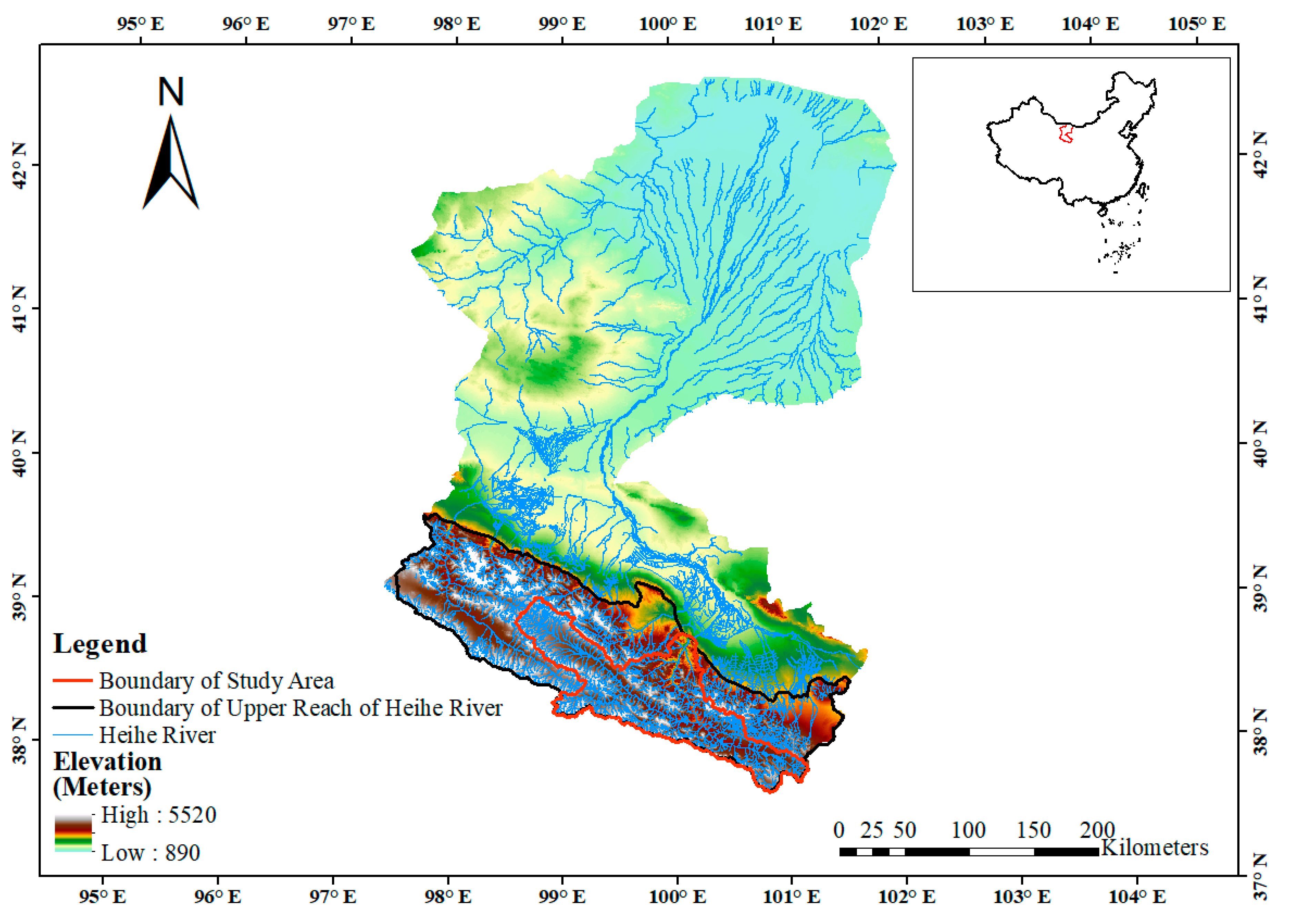
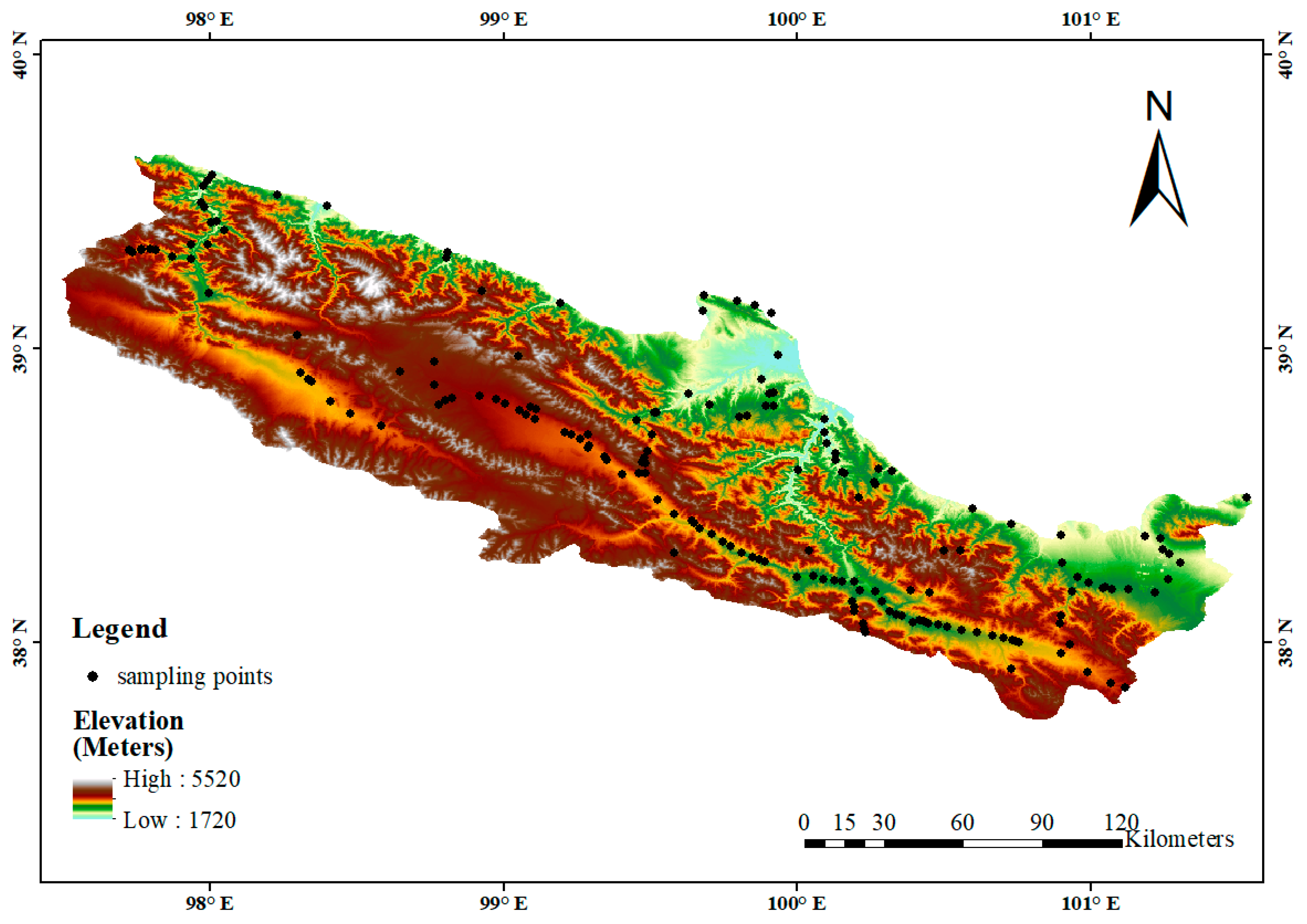
2. The Study Area
3. Materials and Methods
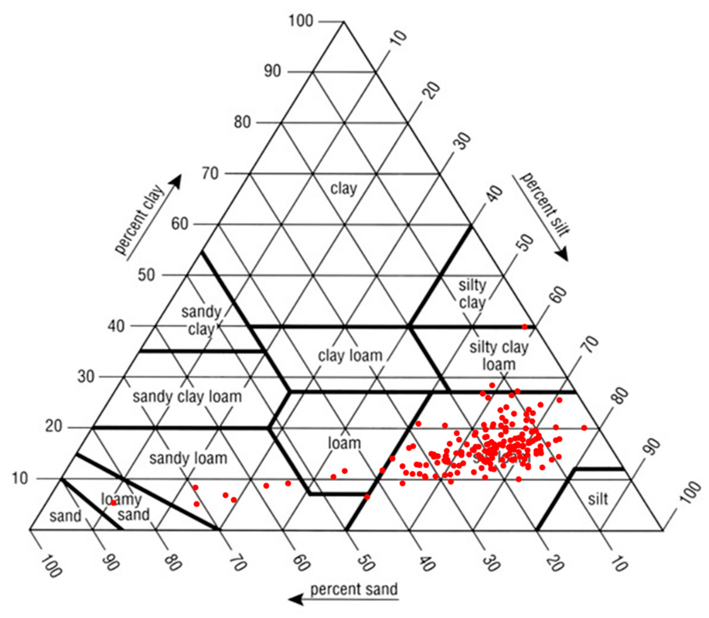
3.1. Soil Sampling
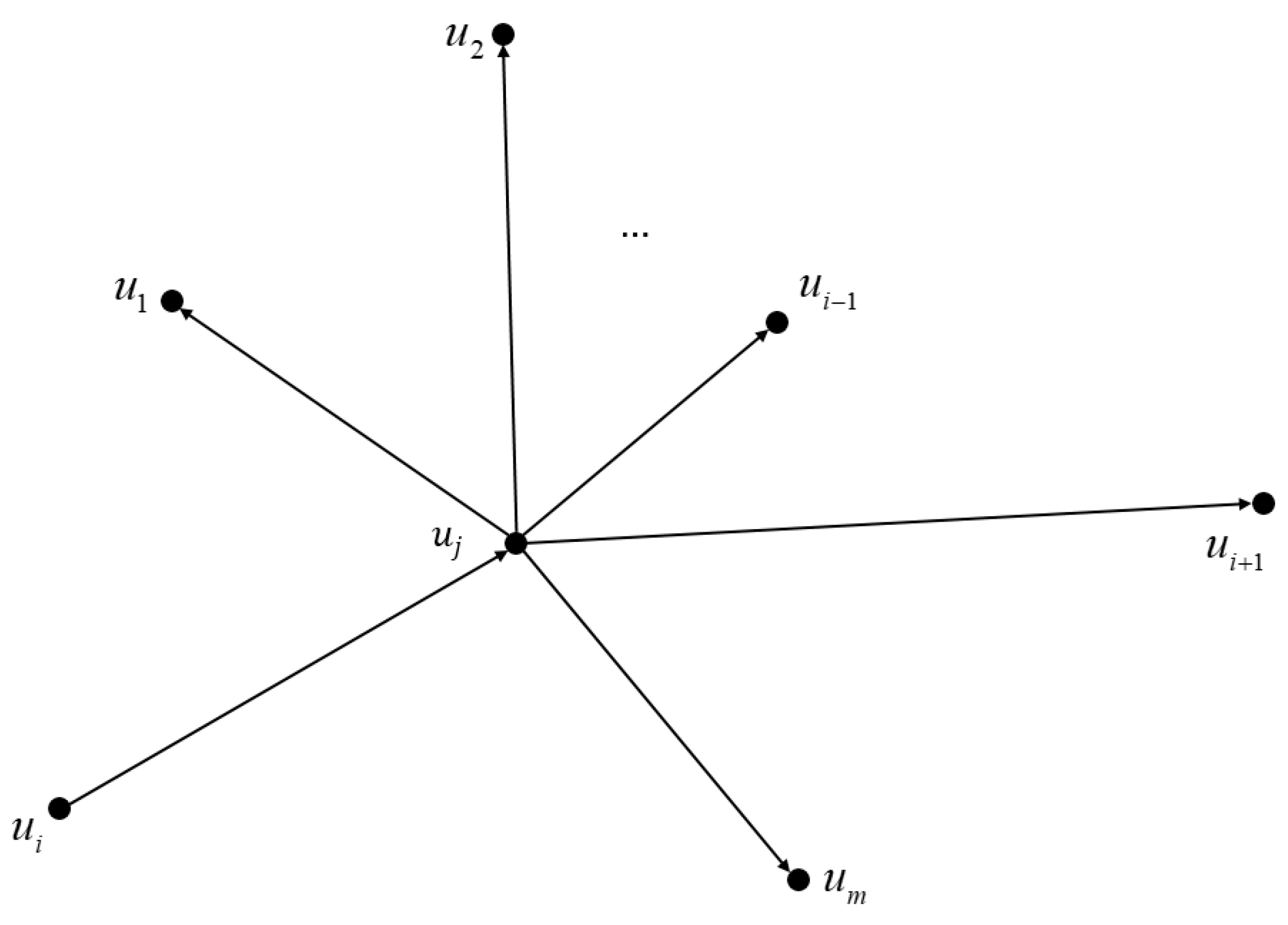
3.2. The MCRF Method
3.3. The Ordinary Kriging Method
3.4. Evaluation Criteria
4. Results
4.1. The Search Radiuses
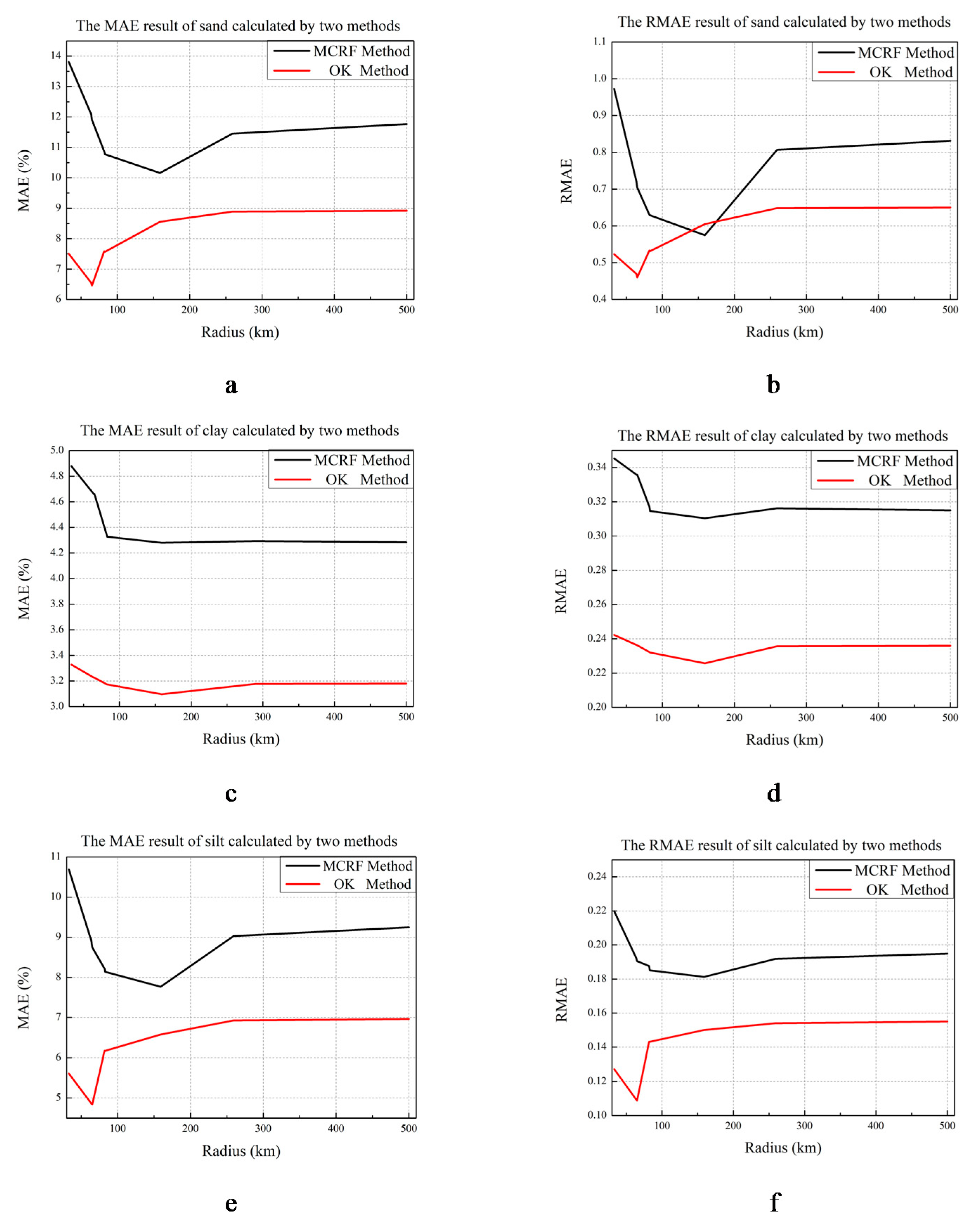
4.2. The Performance Comparison of the MCRF and OK Methods in Calculating Individual Sand, Silt, and Clay Component
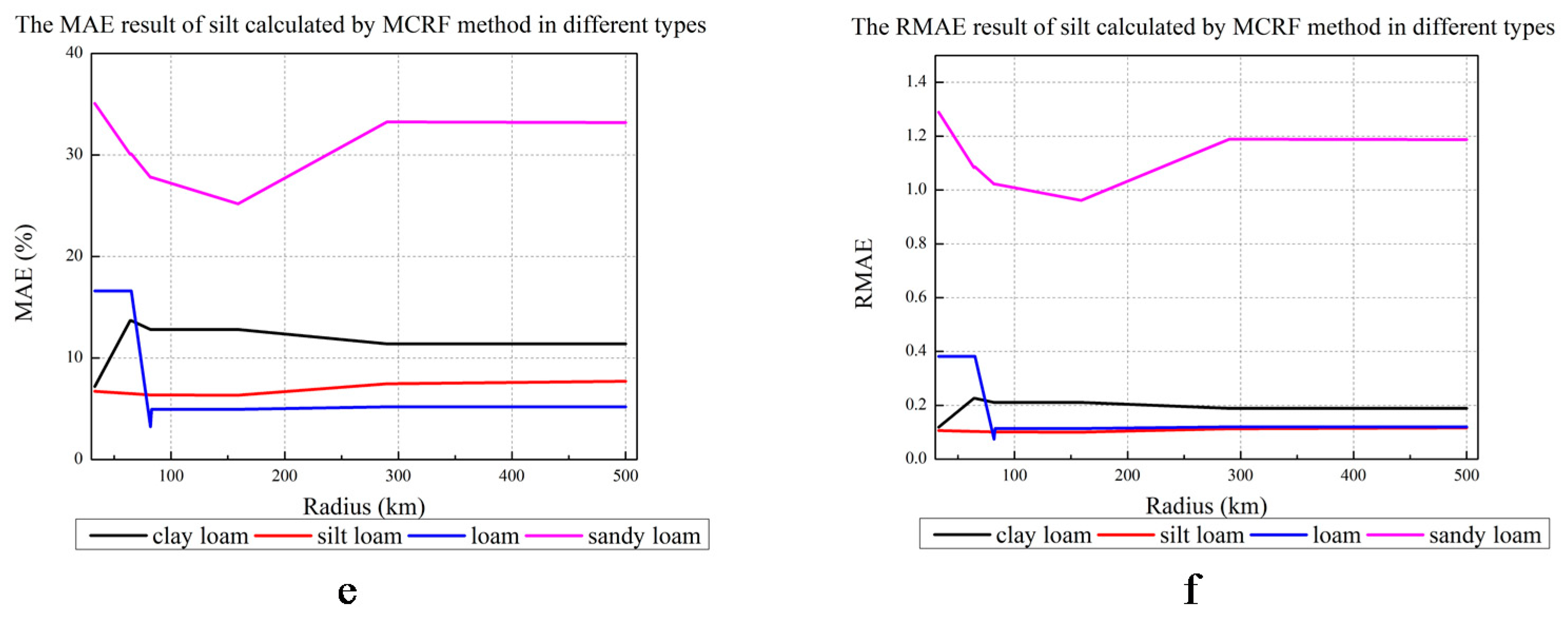
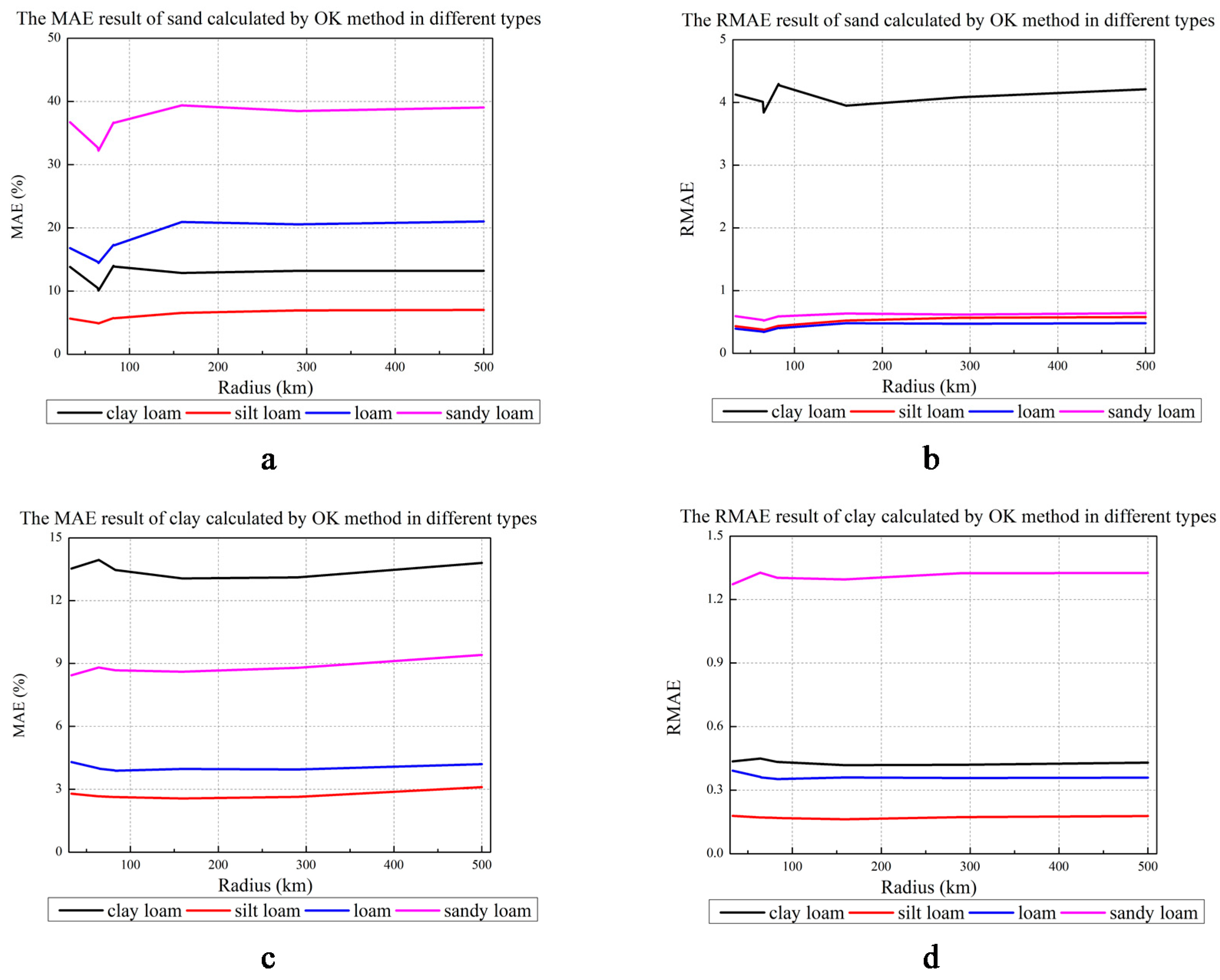
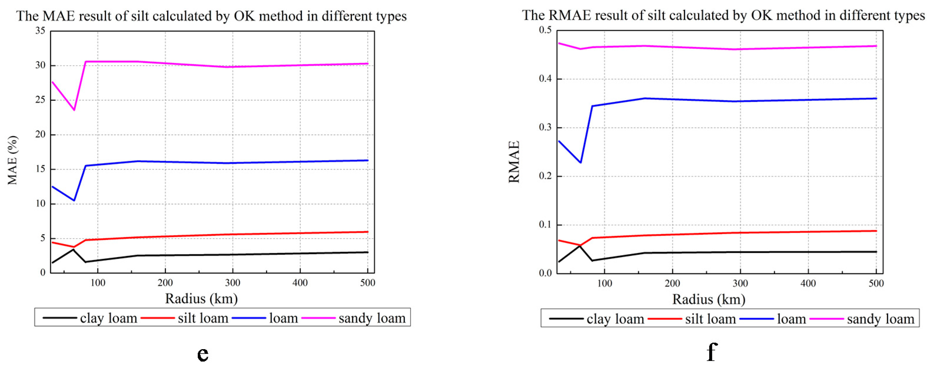
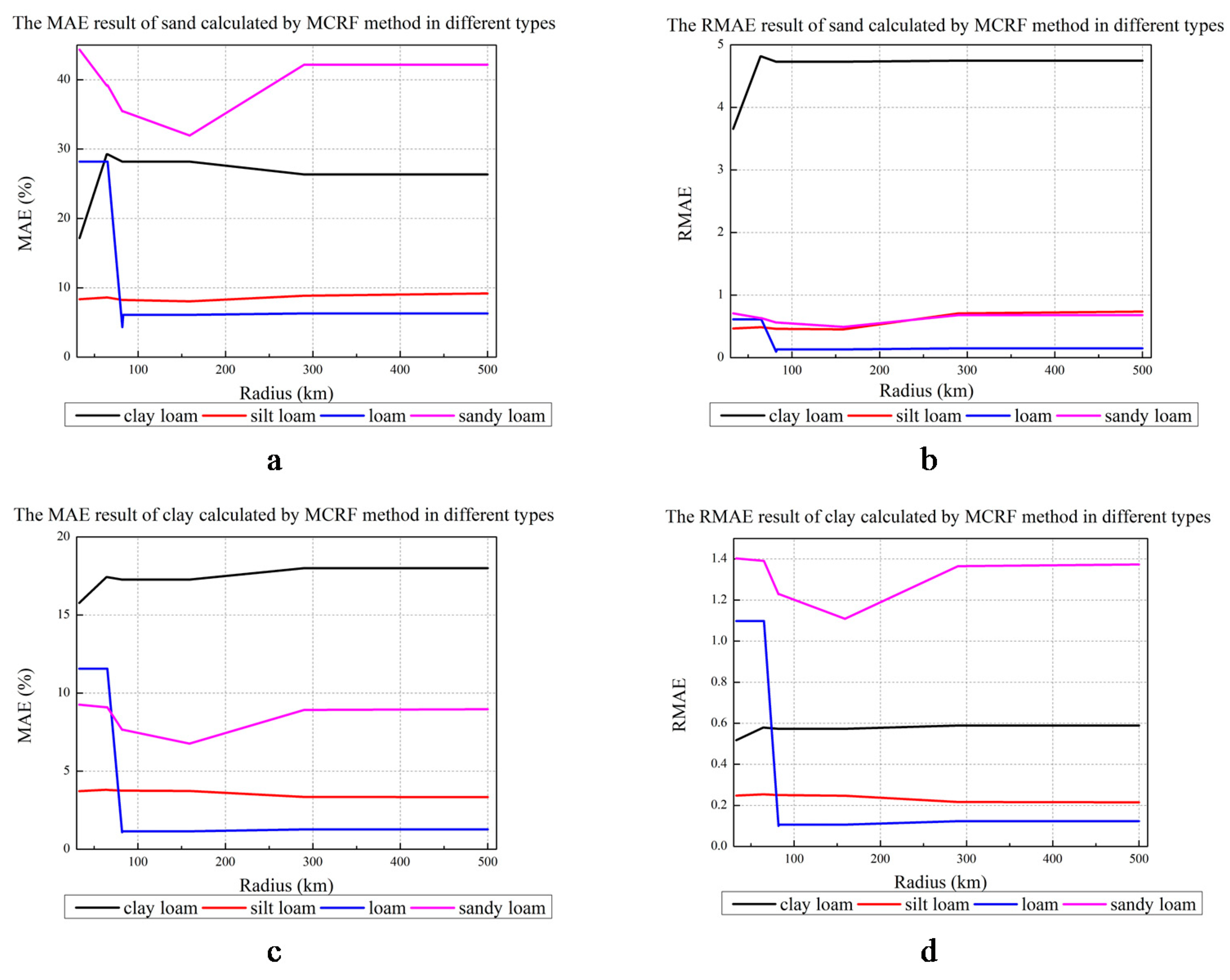
4.3. The Performance of Both the MCRF and OK Methods in Calculating Different Soil Texture Types
5. Discussion
5.1. The Impacts of Different Computation Mechanisms
5.2. The Impacts of Sampling Point Distribution
5.3. The Impacts of Sampling Point Variability
6. Conclusions
Author Contributions
Funding
Acknowledgments
Conflicts of Interest
References
- Zhao, M.Z.; Chow, T.L.; Rees, H.W.; Yang, Q.; Xing, Z.; Meng, F.R. Predict soil texture distributions using an artificial neural network model. Comput. Electron. Agric. 2009, 65, 36–48. [Google Scholar] [CrossRef]
- Silva, M.; Poly, F.; Guillaumaud, N.; van Elsas, J.D.; Salles, J.F. Fluctuations in ammonia oxidizing communities across agricultural soils are driven by soil structure and pH. Front. Microbiol. 2012, 3, 77. [Google Scholar]
- Fernandez-Illesca, C.P.; Porporato, A.; Liao, F.; Rodriguez-Iturbe, I. The ecohydrological role of soil texture in a water-limited ecosystem. Water Resour. Res. 2001, 37, 2863–2872. [Google Scholar] [CrossRef] [Green Version]
- Mulder, V.L.; de Bruin, S.; Schaepman, M.E.; Mayr, T.R. The use of remote sensing in soil and terrain mapping—A review. Geoderma 2011, 162, 1–19. [Google Scholar] [CrossRef]
- Cotching, W.E.; Oliver, G.; Downie, M.; Corkrey, R.; Doyle, R.B. Land use and management influences on surface soil organic carbon in Tasmania. Soil Res. 2013, 51, 615–630. [Google Scholar] [CrossRef]
- Adhikari, K.; Kheir, R.B.; Greve, M.B.; Bøcher, P.K.; Malone, B.P.; Minasny, B.; McBratney, A.B.; Greve, M.H. High-resolution 3-D mapping of soil texture in Denmark. Soil Sci. Soc. Am. J. 2013, 77, 860–876. [Google Scholar] [CrossRef]
- Akpa, S.I.C.; Odeh, I.O.A.; Bishop, T.F.A.; Hartemink, A.E. Digital mapping of soil particle-size fractions for Nigeria. Soil Sci. Soc. Am. J. 2014, 78, 1953–1966. [Google Scholar] [CrossRef]
- Lu, L.; Liu, C.; Li, X.; Ran, Y. Mapping the soil texture in the Heihe River Basin based on fuzzy logic and data fusion. Sustainability 2017, 9, 1246. [Google Scholar] [CrossRef]
- Rad, M.R.P. Spatial variability of soil texture fractions and pH in a flood plain (case study from eastern Iran). Catena 2018, 160, 275–281. [Google Scholar]
- Sayão, V.M.; Demattê, J.A.M. Soil texture and organic carbon mapping using surface temperature and reflectance spectra in Southeast Brazil. Geoderma Reg. 2018, 14, e00174. [Google Scholar] [CrossRef]
- Li, W.; Zhang, C.; Burt, J.E.; Zhu, A.; Feyen, J. Two-dimensional Markov chain simulation of soil class spatial distribution. Soil Sci. Soc. Am. J. 2004, 68, 1479–1490. [Google Scholar] [CrossRef]
- Oberthür, T.; Goovaerts, P.; Dobermann, A. Mapping soil texture classes using field textuing, particle size distribution and local knowledge by both conventional and geostatisical methods. Eur. J. Soil Sci. 2015, 50, 457–479. [Google Scholar] [CrossRef] [Green Version]
- Liu, F.; Geng, X.; Zhu, A.X.; Fraser, W.; Waddell, A. Soil texture mapping over low relief areas using land surface feedback dynamic patterns extracted from MODIS. Geoderma 2012, 171–172, 44–52. [Google Scholar] [CrossRef]
- Niang, M.; Nolin, M.C.; Jégo, G.; Perron, I. Digital Mapping of Soil Texture Using RADARSAT-2 Polarimetric Synthetic Aperture Radar Data. Soil Sci. Soc. Am. J. 2014, 78, 673. [Google Scholar] [CrossRef]
- Gao, Y.H.; Chen, F.; Barlage, M.; Liu, W.; Cheng, G.; Li, X. Enhancement of land surface information and its impact on atmospheric modeling in the Heihe River Basin, Northwest China. J. Geophys. Res. Atmos. 2008, 113, D20. [Google Scholar] [CrossRef]
- Wang, D.; Zhang, G.; Pan, X.; Zhao, Y.; Zhao, M.; Wang, G. Mapping Soil Texture of a Plain Area Using Fuzzy-c-Means Clustering Method Based on Land Surface Diurnal Temperature Difference. Pedosphere 2012, 22, 394–403. [Google Scholar] [CrossRef]
- Yang, R.; Liu, F.; Zhang, G.; Zhao, Y.; Li, D.; Yang, J.; Yang, F.; Yang, F. Mapping Soil Texture Based on Field Soil Moisture Observations at a High Temporal Resolution in an Oasis Agricultural Area. Pedosphere 2016, 26, 699–708. [Google Scholar] [CrossRef]
- Delabri, M.; Afraslab, P.; Loiskandl, W. Geostatistical analysis of soil texture fractions on the field scale. Soil Water Res. 2011, 6, 173–189. [Google Scholar] [CrossRef] [Green Version]
- Mercedes, R.D.; Thomas, G.O.; Dominique, A.; Blandine, L.; Jean-Baptiste, P.; Christian, W.; Nicolas, P.A.S. Prediction of soil texture using descriptive statistics and area-to-point Kriging in Region Centre (France). Geoderma Reg. 2016, 279–292. [Google Scholar]
- Bishop, T.F.A.; McBratney, A.B. A comparison of prediction methods for the creation of field-extent soil property maps. Geoderma 2001, 103, 149–160. [Google Scholar] [CrossRef]
- Da César, S.C.; de Waldir, C.J.; Silvio, B.B.; Filho, B.C. Spatial prediction of soil surface texture in a semiarid region using random forest and multiple linear regressions. Catena 2016, 139, 232–240. [Google Scholar]
- Wiesmeier, M.; Barthold, F.; Blank, B.; Kögel-Knabner, I. Digital mapping of soil organic matter stocks using Random Forest modeling in a semi-arid steppe ecosystem. Plant Soil 2011, 340, 7–24. [Google Scholar] [CrossRef]
- Ließ, M.; Glaser, B.; Huwe, B. Uncertainty in the spatial prediction of soil texture comparison of regression tree and Random Forest models. Geoderma 2012, 170, 70–79. [Google Scholar] [CrossRef]
- Mckenzie, N.J.; Ryan, P.J. Spatial prediction of soil properties using environmental correlation. Geoderma 1999, 89, 67–94. [Google Scholar] [CrossRef]
- Burgess, T.M.; Webster, R. Optimal interpolation and isarithmic mapping of soil properties: I. The variogram and punctual Kriging. J. Soil Sci. 1980, 31, 315–331. [Google Scholar] [CrossRef]
- Goovaerts, P. Geostatistics for Natural Resources Evaluation; Oxford University Press: New York, NY, USA, 1997; Volume 9. [Google Scholar]
- Liao, K.; Xu, S.; Wu, J.; Zhu, Q. Spatial estimation of surface soil texture using remote sensing data. Soil Sci. Plant Nutr. 2013, 59, 488–500. [Google Scholar] [CrossRef] [Green Version]
- Zhang, S.W.; Shen, C.Y.; Chen, X.; Ye, H.; Huang, Y.; Lai, S. Spatial interpolation of soil texture using compositional Kriging and regression Kriging with consideration of the characteristics of compositional data and environment variables. J. Integr. Agric. 2013, 12, 1673–1683. [Google Scholar] [CrossRef]
- Journel, A.G.; Huijbregts, C.J. Mining Geostatistics; Academic Press: New York, NY, USA, 1978. [Google Scholar]
- Isaaks, E.H.; Srivastava, R.M. An Introduction to Applied Geostatistics; Oxford University Press: New York, NY, USA, 1989. [Google Scholar]
- Voltz, M.; Lagacherie, P.; Louchart, X. Predicting soil properties over a region using sample information from a mapped reference area. Eur. J. Soil Sci. 1997, 48, 19–30. [Google Scholar] [CrossRef]
- Heuvelink, G.B.M.; Bierkens, M.F.P. Combining soil maps with interpolations from point observations to predict quantitative soil properties. Geoderma 1992, 55, 1–15. [Google Scholar] [CrossRef]
- McBratney, A.B.; Odeh, I.O.A.; Bishop, T.F.A.; Dunbar, M.S.; Shatar, T.M. An overview of pedometric techniques for use in soil survey. Geoderma 2000, 97, 293–327. [Google Scholar] [CrossRef]
- Thattai, D.; Islam, S. Spatial analysis of remotely sensed soil moisture data. J. Hydrol. Eng. 2000, 5, 386–392. [Google Scholar] [CrossRef]
- Richard, S. Basics of Applied Stochastic Processes; Springer Science & Business Media: Berlin, Germany, 2009; p. 2. ISBN 978-3-540-89332-5. [Google Scholar]
- Gagniuc, P.A. Markov Chains: From Theory to Implementation and Experimentation; John Wiley & Sons: Hoboken, NJ, USA, 2017; pp. 1–8. ISBN 978-1-119-38755-8. [Google Scholar]
- Shamshad, A.; Bawadi, M.A.; Hussin, W.M.A.W.; Majid, T.A.; Sanusi, S.A.M. First and second order Markov chain models for synthetic generation of wind speed time series. Energy 2005, 30, 693–708. [Google Scholar] [CrossRef]
- Wootton, J.T. Markov chain models predict the consequences of experimental extinctions. Ecol. Lett. 2010, 7, 653–660. [Google Scholar] [CrossRef]
- Li, W.; Zhang, C. Application of transiograms to Markov chain simulation and spatial uncertainty assessment of land-cover classes. GISci. Remote Sens. 2005, 42, 297–319. [Google Scholar] [CrossRef]
- Li, W.; Zhang, C. A generalized Markov chain approach for conditional simulation of categorical variables from grid samples. Trans. GIS 2006, 10, 651–669. [Google Scholar] [CrossRef]
- Li, W.; Zhang, C. A Random-path Markov chain algorithm for simulating categorical soil variables from random point samples. Soil Sci. Soc. Am. J. 2007, 71, 656–668. [Google Scholar] [CrossRef]
- Pan, Q. The Water Resources of Heihe Watershed; Yellow River Conservation Press: Zhengzhou, China, 2001. (In Chinese) [Google Scholar]
- Zhang, L.; Jin, X.; He, C.; Zhang, B.; Zhang, X.; Li, J.; Zhao, C.; Tian, J.; DeMarchi, C. Comparison of SWAT and DLBRM for hydrological modeling of a mountainous watershed in arid Northwest China. J. Hydrol. Eng. 2016, 21, 04016007. [Google Scholar] [CrossRef]
- Li, Z.; Xu, Z.; Shao, Q.; Yang, J. Parameter estimation and uncertainty analysis of SWAT model in upper reaches of the Heihe river basin. Hydrol. Process. 2009, 23, 2744–2753. [Google Scholar] [CrossRef]
- Jin, X.; Zhang, L.; Gu, J.; Zhao, C.; Tian, J.; He, C. Modeling the Impacts of Spatial Heterogeneity in Soil Hydraulic Properties on Hydrologic Process in the Upper Reach of the Heihe River in the Qilian Mountains, Northwest China. Hydrol. Process. 2015. [Google Scholar] [CrossRef]
- Nachtergaele, F.; Velthuized, H.V.; Verelst, L. Harmonized World Soil Database (Version 1.1); FAO: Rome, Italy; IIASA: Laxenburg, Austria, 2009. [Google Scholar]
- Shi, X.Z.; Yu, D.S.; Warner, E.D.; Pan, X.Z.; Sun, X.; Petersen, G.W.; Gong, Z.G.; Lin, H. Cross reference system for translating between genetic soil classification of China and soil taxonomy. Soil Sci. Soc. Am. J. 2006, 70, 78–83. [Google Scholar] [CrossRef]
- Shi, X.Z.; Yu, D.S.; Yang, G.X.; Wang, H.J.; Sun, W.X.; Du, G.H.; Gong, Z.T. Cross-reference benchmarks for correlating the genetic soil classification of China and Chinese soil taxonomy. Pedosphere 2006, 16, 147–153. [Google Scholar] [CrossRef]
- Kerry, R.; Oliver, M. Variograms of ancillary data to aid sampling for soil surveys. Precis. Agric. 2003, 4, 261–278. [Google Scholar] [CrossRef]
- López-Granados, F.; Jurado-Expósito, M.; Pena-Barragan, J.M. García-Torres, L. Using geostatistical and remote sensing approaches for mapping soil properties. Eur. J. Agron. 2005, 23, 279–289. [Google Scholar] [CrossRef]
- Jensen, J.R. Introductory Digital Image Processing, 3rd ed.; Prentice Hall: Upper Saddle River, NJ, USA, 2004. [Google Scholar]
- Soil Survey Staff. Soil Taxonomy: A Basic System of Soil Classification for Making and Interpreting Soil Surveys, 2nd ed.; Agricultural Handbook 436; Natural Resources Conservation Service, USDA: Washington, DC, USA, 1999; p. 869.
- Tian, J.; Zhang, B.; He, C.; Yang, L. Variability of Soil Hydraulic Conductivity and Soil Hydrological Response under Different Land Cover in the Mountainous Area of the Heihe River Watershed, Northwest China. Land Degrad. Dev. 2017, 28, 1437–1449. [Google Scholar] [CrossRef]
- Li, W. Markov Chain Random Fields for Estimation of Categorical Variables. Math Geol. 2007, 39, 321–335. [Google Scholar] [CrossRef]
- Elfeki, A.M.; Dekking, F.M. A Markov chain model for subsurface characterization: Theory and applications. Math. Geol. 2001, 33, 569–589. [Google Scholar]
- Zhang, J.X.; Yao, N. The geostatistical framework for spatial prediction. Geo-Spat. Inf. Sci. 2008, 10, 44–50. [Google Scholar] [CrossRef]
- Sakata, S.; Ashida, F.; Zako, M. Structural optimization using Kriging approximation. Comput. Methods Appl. Mech. Eng. 2003, 192, 923–939. [Google Scholar] [CrossRef]
- Sakata, S.; Ashida, F. Integral estimation with the ordinary Kriging method using the Gaussian semivariogram function. Int. J. Numer. Meth. Biomed. Eng. 2011, 27, 1235–1251. [Google Scholar] [CrossRef]
- Legates, D.R.; McCabe, G.J. Evaluating the use of “goodness-of-fit” measures in hydrologic and hydroclimatic model validation. Water Resour. Res. 1999, 35, 233–241. [Google Scholar] [CrossRef]
- Krause, P.; Boyle, D.P.; Bäse, F. Comparison of different efficiency criteria for hydrological model assessment. Adv. Geosci. 2005, 5, 89–97. [Google Scholar]
- Groenigen, J.W.V. The influence of variogram parameters on optimal sampling schemes for mapping by kriging. Geoderma 2000, 97, 223–236. [Google Scholar] [CrossRef]
- Yamamoto, J.K. Correcting the smoothing effect of ordinary kriging stimates. Math Geol. 2005, 37, 69–94. [Google Scholar] [CrossRef]
- Meul, M.; Meirvenne, M.V. Kriging soil texture under different types of nonstationarity. Geoderma 2003, 112, 217–233. [Google Scholar] [CrossRef]
- Yasrebi, J.; Saffari, M.; Fathi, H.; Karimian, N.; Moazallahi, M.; Gazni, R. Evaluation and comparison of Ordinary Kriging and Inverse Distance Weighting methods for prediction of spatial variability of some soil chemical parameters. Res. J. Biol. Sci. 2009, 4, 93–102. [Google Scholar]
- Bland, J.M.; Altman, D.G. Statistics notes: Measurement error. BMJ 1996, 312, 1654. [Google Scholar] [CrossRef] [PubMed]


| Texture Type | Conditions | Percentage |
|---|---|---|
| clay loam | (27% ≤ clay < 40%) and (20%< sand ≤ 45%) | 2.247% |
| silt loam | ((silt ≥ 50% and (12%≤ clay < 27%)) or ((50% ≤ silt < 80%) and clay < 12%)) | 88.764% |
| loam | (7 %≤ clay < 27%) and (28%≤ silt < 50%) and (sand ≤ 52%)) | 2.247% |
| sandy loam | ((7% ≤ clay < 20%) and (sand > 52%) and ((silt + 2 × clay) ≥ 30%)) or (clay < 7% and silt < 50% and (silt + 2 × clay) ≥ 30%) | 6.180% |
| loamy sand | (silt + 1.5 × clay ≥ 15%) and (silt + 2 × clay < 30%)) | 0.562% |
| MAE | RMAE | ||||
|---|---|---|---|---|---|
| Soil Texture Types | OK | MCRF | OK | MCRF | |
| Clay loam | Sand | 10.1021 | 28.1851 | 3.8387 | 4.7396 |
| Silt | 3.2202 | 12.8048 | 0.0542 | 0.2111 | |
| Clay | 13.9221 | 17.2663 | 0.4489 | 0.5732 | |
| Loam | Sand | 14.4521 | 6.1023 | 0.3402 | 0.13401 |
| Silt | 10.5080 | 4.9518 | 0.2279 | 0.1139 | |
| Clay | 3.9748 | 1.1504 | 0.3601 | 0.1068 | |
| Sandy loam | Sand | 32.2152 | 31.9541 | 0.5221 | 0.4912 |
| Silt | 23.5802 | 25.1850 | 0.4619 | 0.9619 | |
| Clay | 8.7981 | 6.7691 | 1.3259 | 1.1093 | |
| Silt loam | Sand | 4.8970 | 8.0348 | 0.3751 | 0.4531 |
| Silt | 3.7931 | 6.3381 | 0.0588 | 0.1012 | |
| Clay | 2.6656 | 3.7331 | 0.1708 | 0.2468 | |
| Radius (km) | 33 | 64 | 65 | 82 | 83 | 159 | 290 | 500 |
|---|---|---|---|---|---|---|---|---|
| Density((km2)−1) | 0.0025 | 0.0022 | 0.0023 | 0.0020 | 0.0020 | 0.0015 | 0.0006 | 0.0002 |
| Radiuses (km) | 33 | 64 | 65 | 82 | 83 | 159 | 290 | 500 |
|---|---|---|---|---|---|---|---|---|
| Clay loam | 14.6 | 5.8 | 5.7 | 3.6 | 3.5 | 3.2 | 1 | 0.3 |
| Loam | 0 | 0 | 0 | 9.5 | 9.2 | 2.5 | 0.8 | 0.2 |
| Sandy loam | 0 | 2.2 | 3.2 | 2.7 | 2.6 | 4.7 | 2 | 0.7 |
© 2018 by the authors. Licensee MDPI, Basel, Switzerland. This article is an open access article distributed under the terms and conditions of the Creative Commons Attribution (CC BY) license (http://creativecommons.org/licenses/by/4.0/).
Share and Cite
Li, J.; Zhang, L.; He, C.; Zhao, C. A Comparison of Markov Chain Random Field and Ordinary Kriging Methods for Calculating Soil Texture in a Mountainous Watershed, Northwest China. Sustainability 2018, 10, 2819. https://doi.org/10.3390/su10082819
Li J, Zhang L, He C, Zhao C. A Comparison of Markov Chain Random Field and Ordinary Kriging Methods for Calculating Soil Texture in a Mountainous Watershed, Northwest China. Sustainability. 2018; 10(8):2819. https://doi.org/10.3390/su10082819
Chicago/Turabian StyleLi, Jinlin, Lanhui Zhang, Chansheng He, and Chen Zhao. 2018. "A Comparison of Markov Chain Random Field and Ordinary Kriging Methods for Calculating Soil Texture in a Mountainous Watershed, Northwest China" Sustainability 10, no. 8: 2819. https://doi.org/10.3390/su10082819