Some Novel Bayesian Model Combination Schemes: An Application to Commodities Prices

Faculty of Economic Sciences, University of Warsaw, 00-241 Warsaw, Poland
Sustainability 2018, 10(8), 2801; https://doi.org/10.3390/su10082801
Submission received: 10 July 2018
/
Revised: 2 August 2018
/
Accepted: 3 August 2018
/
Published: 7 August 2018
Abstract
:Forecasting commodities prices on vividly changing markets is a hard problem to tackle. However, being able to determine important price predictors in a time-varying setting is crucial for sustainability initiatives. For example, the 2000s commodities boom gave rise to questioning whether commodities markets become over-financialized. In case of agricultural commodities, it was questioned if the speculative pressures increase food prices. Recently, some newly proposed Bayesian model combination scheme has been proposed, i.e., Dynamic Model Averaging (DMA). This method has already been applied with success in certain markets. It joins together uncertainty about the model and explanatory variables and a time-varying parameters approach. It can also capture structural breaks and respond to market disturbances. Secondly, it can deal with numerous explanatory variables in a data-rich environment. Similarly, like Bayesian Model Averaging (BMA), Dynamic Model Averaging (DMA), Dynamic Model Selection (DMS) and Median Probability Model (MED) start from Time-Varying Parameters’ (TVP) regressions. All of these methods were applied to 69 spot commodities prices. The period between Dec 1983 and Oct 2017 was analysed. In approximately 80% of cases, according to the Diebold–Mariano test, DMA produced statistically significant more accurate forecast than benchmark forecasts (like the naive method or ARIMA). Moreover, amongst all the considered model types, DMA was in 22% of cases the most accurate one (significantly). MED was most often minimising the forecast errors (28%). However, in the text, it is clarified that this was due to some specific initial parameters setting. The second “best” model type was MED, meaning that, in the case of model selection, relying on the highest posterior probability is not always preferable.
1. Introduction
During the 2000s, a commodities price boom was observed. Naturally, this led to the question of what was the purpose of such price spikes. Some of the hypotheses were based on the growing financialization of commodities markets. In other words, it was observed since the 1990s that the links between commodities prices and equity markets become more and more tight. For the previous periods, more research emphasis was put on the fundamental factors like supply and demand, etc.
The problem of sustainability is clearly seen in agricultural commodities. Especially in recent years, this has been noticed not only by the final goods’ consumers, but also by the producers. Nevertheless, such initiatives spread over whole commodities’ markets. Sustainable products might generate more stable revenues to producers, stakeholders can reduce their risk exposure, consumers become more aware of natural resources. Within this context, it seems interesting to construct a tool which would be able to model commodities prices, and which would be able to deal with variable uncertainty, as well as having its initial feature of time-varying coefficients. These adaptive abilities might make it a superior method in a highly volatile market background.
Forecasting commodity prices is a very difficult task. The reason for this is that the structure and the behaviour of commodities markets can be quite complex. For example, certain nonlinear effects can emerge, which, furthermore, can lead to chaotic behaviours. However, even without incorporating the developed conceptual machinery, many previous studies indicated that, in different time periods, different factors are the leading determinants of the prices of various commodities [1,2,3]. Therefore, in some periods, certain models work quite well, but, in the other periods, some other models work much better.
In other words, when a longer time horizon is analysed, the uncertainty about the true model arises (i.e., the set of predictors). However, except for the model uncertainty, there are strong arguments to also allow for time-varying parameters in the considered models (i.e., to allow regression coefficients, if the regression models are considered, to vary in time). This corresponds to possible changes in the strength (or even in the direction) of the impact of a predictor on the considered commodity price.
Naturally, this problem can be tackled with the Bayesian methods, and indeed, Bayesian Model Averaging (BMA) and its slight modification, i.e., Bayesian Model Selection (BMS), have been recently used in various branches of economics with a success. In order to extend this method, recently, a new framework was proposed [4]. Dynamic Model Averaging (DMA) allows for both time-varying: the state space of the model and its parameters (i.e., regression coefficients). Moreover, the final DMA forecast is computed as a weighted forecast from the predictions of all included models. However, the weights used are updated recursively with respect to the quality of forecast (i.e., predictive density) produced by the models in preceding periods.
A few years after presenting the theoretical foundations of this method, a rapid interest in it for the purpose of economics and finance can be observed. Of course, most of the published results provide arguments in favour of DMA, which can beat some alternative forecasts. Therefore, the first aim of this paper is to report a unified and consistent application of DMA to possibly large number of commodities. In addition, to provide some hints about the “calibration” of the initial parameters for this method. In particular, 69 time-series provided by The World Bank [5] were taken. The second aim of this paper is to compare DMA with the other, similar Bayesian methods. In other words, to verify whether DMA is superior to the previously proposed averaging method, and whether the model averaging itself improves the forecast accuracy in the case of commodity prices. Following Gargano and Timmermann [6], this study is based on macroeconomic and financial predictors. The second motivation behind using macroeconomic and financial predictors is to obtain a common set of predictors and use quite numerous time-series of commodity prices.
Indeed, this paper tries to fill some literature gaps. Contrary to previous DMA studies focusing on one approach to a relatively small number of independent variables (for example, [7,8,9], here, applying a similar pattern to possibly many commodities is attempted to see if some pattern will be recovered. However, this is not a somehow veiled data dredging. It is obvious that a more tailored data set of predictors can result in higher forecast accuracy. On the other hand, if certain research argues that some macroeconomic and financial variables (therefore common ones for different commodities) can serve as satisfactory commodities prices’ predictors [6], then it is worth checking if DMA can produce more accurate forecasts in comparison to the existing methods. In other words, the results of this paper might provide some arguments that, indeed, DMA forecast combination scheme is highly beneficial. However, they might also bring some shadow on DMA and provide rather the following argument: the already reported success of DMA (see, for example [10,11,12]) is mostly due to the suitable choice of predictors (and analysed period), not due to the method itself.
In the next section, a brief overview of the results already obtained with DMA is presented. In addition, the short review motivating the selection of possible commodity price predictors is given. It is also discussed why model averaging can lead to better forecast performance. Next, data are described in details. Furthermore, a short overview of DMA and other methods used in this research is sketched. Next, the results are presented and discussed. Moreover, some preliminary results, motivating the selection of the initial parameters for the main DMA models are discussed. This is believed to be of some help for future researches based on DMA methods. For the reader’s convenience, the list of abbreviations is given at the end of the paper.
2. Literature Review
This section is divided into two parts. First, which fields DMA has already been applied in is summarized. Next, a few recent research papers are presented with a stress put on the novelty of the methodology. Finally, which variables can be initially considered as potentially useful predictors in the construction of the econometric model of the selected commodities is presented.
2.1. Dynamic Model Averaging
DMA has already been applied to model various time-series and, in the case of commodities: copper, crude oil and gold. Aye et al. [13] used DMA to forecast gold price returns. Most of the predictors were chosen on the basis of a recursive principal component analysis. Both DMA and DMS were found to be superior to BMA and the naive forecast. In addition, Baur et al. [10] found similar conclusions. Risse and Ohl [14] compared the DMA improved by the Dynamic Occam’s Window of Onorante and Raftery [15] with the original DMA and some other machine learning techniques. They found that such a modification produces the best forecasts of gold prices.
Buncic and Moretto [7] found that DMA and DMS produces more accurate forecasts than the historical mean and the naive forecast in case of copper price. They used as predictors both macroeconomic and financial variables as well as fundamental factors specific for copper. For example, supply and demand, returns from specific stocks (firms heavy depending on commodity market), etc. Drachal [8] found that, in case of crude oil prices, it is quite hard to produce a statistically significant more accurate forecast than the naive one and autoregressive models with DMA. However, these benchmark forecasts were also not found to be superior to DMA and DMS. On the other hand, Naser [11] used DMA with a large set of predictors, and concluded that DMA outperforms alternative models as well as forecasts based on future prices.
Baxa et al. [16] successfully applied DMA to forecast inflation in G7 countries. Similarly, inflation was modeled with DMA by Del Negro et al. [17]. However, Di Filippo [18] concluded that, in the case of inflation, DMS produced better forecasts than DMA. In other words, model selection was more appropriate than model averaging. Ferreira and Palma [19] concluded that, in the case of modeling, the Brazilian inflation DMA behaves very well. These studies were usually done in the context of the generalized Phillips curve [20]. Indeed, such studies were usually made in a general macroeconomic context. For example, the economic growth was also modeled with DMA [21,22].
DMA was also used in real property markets. Bork and Moller [23] used it (and also DMS) to forecast house prices in the US. Risse and Kern [9] found DMA a superior method for forecasting house prices in the Euro area countries. Wei and Cao [12] applied DMA to model house prices in major Chinese cities. They also implemented a slight modification of the original DMA method. They concluded that this method is more accurate than BMA, information-theoretic averaging, and that, indeed, the time-varying weights’ scheme significantly improves the forecast quality.
De Bruyn et al. [24] applied DMA to forecast South African rand to the US dollar exchange rate and to the UK pound. The comparison was made with BMA and the random walk model. DMA was found to be superior to the benchmark models. Gupta et al. [25] examined with DMA the growth of China’s foreign exchange reserves. DMA and DMS were found superior to the random walk, recursive OLS-AR(1), recursive OLS and BMA.
DMA was also found useful in modeling carbon prices [26]. Liu et al. [27] used this method to forecast the realized range-based volatility. They concluded that time-varying weights indeed generate more accurate forecasts. Similar conclusions were derived by Wang et al. [28]. Finally, Naser and Alaali [29] applied a DMA framework to model the US stock prices’ returns.
2.2. Other Models
Indeed, the fact that forecast combination can lead to a more accurate forecast than the selection of one model is both an empirical and theoretically understood fact. The seminal paper in this context was published quite long ago [30]. In case of commodities, the recent findings support averaging over various models [31] as well as the necessity to consider a possibly wide set of predictors [32,33]. However, there are various methods of forecast combinations [34,35] and, yet, within the context of data-rich models, it is natural to focus on the Bayesian methodology [36,37]. This is, for example, due to the fact that, if the number of predictors exceeds the number of observations, then the conventional methods, like OLS are no longer meaningful. On the other hand, the Bayesian formulas are still reasonable in such a case. For example, recently, Lee and Huh [38] proposed some improvements in choosing informative priors for Bayesian models of crude oil price. Yin et al. [39] found that replacing the predictive densities with modified hit ratios in DMA weights’ construction can result in forecast accuracy improvement for oil prices.
Of course, the Bayesian approach is not the only one, which has been applied to commodity prices. However, except for purely classical and fundamental methods like multilinear regression models, etc., various improvements were applied. This was done in order to capture the specific features of the commodity market. For example, Kriechbaumer et al. [40] joined a well-known ARIMA modeling with a wavelet decomposition approach to forecast metals’ prices. The motivation behind using the wavelet analysis was to encompass in the model the cyclical behaviour of metals prices. The obtained framework allowed for increasing the accuracy of one-month ahead forecasts in comparison with the basic ARIMA models. Wang and Sun [41] studied the relationship between oil prices and economic activity and political tension with a structural equation model.
In addition, VAR/VECM methods were applied in the case of bidirectional relationships and the presence of many variables influencing each other. For example, Cross and Nguyen [42] focused on links between China’s economic growth and global oil market fluctuations. They modified the basic VAR methodology to include time-varying parameters’ VAR. Gangopadhyay et al. [43] used VECM methodology to model gold prices in the Indian market, investment decision and inflation.
Gil-Alana et al. [44] used the fractional integration modeling framework to identify structural breaks in metals prices. Kim and Jung [45] improved the predictive ability of standard forecasting models of crude oil prices by a functional partial least squares approach. This was done to deal with multicollinearity of predictors. The framework was compared with principal component regression and least absolute shrinkage and selection operator models.
In the case of a nonconventional approach, neural networks and various types of machine learning techniques are also popular. The review of such methods can be found, for example, in the paper by Hamdi and Aloui [46]. Liu et al. [47] proposed a machine learning algorithm with a decision tree. This method was able to significantly improve copper price forecasting. Zhao et al. [48] focused on the problems with uncertainty about the predictors of oil price. The study was based on almost 200 time-series. They proposed a certain deep learning ensemble approach. They joined an advanced deep neural network model to capture the nonlinearities and an ensemble method to generate multiple training data sets. The implemented algorithm was able to outperform the alternative models.
2.3. Commodities Prices Predictors
In the case of particular commodities prices’ predictors this research follows Gargano and Timmermann [6]. They selected various macroeconomic and financial predictors, which can be common for different commodities. In other words, they were using predictors like interest rates, term spreads, industrial production growth, etc., whereas no specific predictors suitable for just one particular commodity (like, for example, production quotas) was used. Their selection and construction of predictors was much influenced by the studies on stock prices and equity premium forecasting [49]. Of course, this is some kind of a limitation. Indeed, the fundamental factors, for example, inventory quotas, are known to have a significant impact on commodities prices [50]. Nevertheless, the narrowing to macroeconomic and financial predictors is treated as another modeling approach, rather than a sign of ignoring the importance of other predictors. Moreover, such an approach is quite often adapted [51].
It has already been tried to find such common predictors for various commodities in general. For example, Kagraoka [52] within a generalized dynamic factor model concluded that the U.S. inflation rate, the world industrial production, the world stock index and the price of crude oil impact commodities prices. Such methodology was also used by Lübbers and Posch [53] in the analysis of futures prices.
However, even based on a different methodological approach Arango et al. [54], as well as Byrne et al. [55] provided arguments that interest rates significantly impact numerous commodities prices. Alam and Gilbert [56] within a VAR framework concluded that the impact of monetary policy, global economic conditions and U.S. dollar exchange rates are significant for agricultural commodities. However, this study was based also on commodity-specific predictors like inventories quotas, etc. The motivation of this study was similar to the one presented herein: to analyse a big data set of commodities and find common predictors. In case of analysing the impact of exchange rates on commodities prices, a more detailed research was done by, for example, Chen et al. [57].
Much research was also devoted to links between commodities spot and futures prices [58]. However, Hong and Yogo [59] concluded that open interest can serve as an even better proxy than future prices itself. Chen [60] provided arguments that commodity-sensitive stock prices contain an important information for forecasting commodities prices. Indeed, such predictors were used in the already mentioned DMA study of copper prices by Buncic and Moretto [7].
Finally, it should be stressed that, except for various already existing methodologies and continual improvements and development of new ones, forecasting commodities prices remains a very difficult task [61].
Summarizing this considerations, it can be seen that there is a recent rapid increasing interest in the methods combining time-varying parameters and uncertainty about the predictors (or dealing with data-rich models). Economically it is motivated by the increasing complexity of the markets, and time-varying relationships between predictors and commodity prices: both in a sense of the strength and the direction, and even in a sense which predictors are important in particular moments of time. From the mentioned literature of these novel methods, a certain group can be classified, i.e., BMA, BMS, DMA and DMS. All of them emerge from time-varying parameters (TVP) regressions with the Kalman filter. The differences between these methods lie in whether from numerous models the final forecast emerge through the model averaging or model selection—in addition, in case of estimation of the model’s performance, how the weights are updated. It seems that currently there is no paper presenting a unified and consistent approach comparing all these methods for a relatively large set of independent variables (i.e., various spot commodities prices). The current paper is a try to fill this gap.
In particular, it was checked whether DMA indeed outperforms these other Bayesian methods. Secondly, it was checked whether these methods and time-varying regression with all predictors produce significantly more accurate forecasts than ARIMA models or the naive forecast. Once again, it is stressed that the aim was not to focus on some similar set of commodities, but to consider a possibly wide set of commodities and apply a unified methodology to them and see if this methodology leads to some improvement in forecasting. For certain conventional methods, such an approach was reported by Gargano and Timmermann [6].
3. Data
The monthly data between January 1984 and October 2017 were taken. The frequency was chosen as a kind of compromise. Indeed, many macroeconomic data are available even only in quarterly frequency. Therefore, more frequent than monthly data would result in problems with macroeconomic data. On the other hand, too high frequency would need a separate analysis of particular problems connected with very short periods. For example, it can be expected that, in monthly frequency, short-term speculative behaviour is flattened. The period before 1984 was not included due to two facts. First, many commodities prices before that time were not available or their volatilities were so small that the analysis would not be interesting. Secondly, as it is explained further, some variables are missing for certain periods before 1984. Resolving this problem—how to deal with missing observations—would need another discussion and may not seem worth the current research.
Commodities prices were obtained from The World Bank [5]. After trimming the time-series to the above-mentioned period, the remaining time-series which contained missing observations were excluded. As a result, 69 time-series remained. The full list of the analysed commodities is given in Table 1.
The predictors were mostly based on the already discussed papers with a great emphasis on the work of Gargano and Timmermann [6]. Dividend to price ratio (dpr) was taken as the difference between the logarithm of dividends and the logarithm of prices. These data were obtained from Schiller [62]. In particular, prices were taken as S&P Comp. Dividends were transformed to 12-month moving sums. Treasury bill rate (str) was taken as the 3-month treasury bill: secondary market rate (TB3MS) from FRED [63]. Long-term rate of bonds (ltr), because of the lack of exact recent data and problems with methodology, was taken as long-term government bond yields: 10-year, main (including benchmark) for the United States (IRLTLT01USM156N). Term spread (ts) was taken as the difference between the long-term rate of bonds and treasury bill rate. Default return spread (drs) was taken as the difference between long-term corporate bonds yield and treasury bill rate. Long-term corporate bond yield was taken as the index based on bonds with maturities 20-years and above (AAA). Inflation (cpi) was taken as the logarithmic difference of the CPI (Consumer Price Index CPIAUCSL). Industrial production growth (ip) was taken as the logarithmic difference of industrial production (INDPRO). Money stock (m) was taken as the logarithmic difference of M1 money stock (M1SL). In order to measure the economic growth, the classically used GDP was not appropriate because it is available in quarterly—not monthly—frequency. However, it can be found in literature that Kilian [64] global economic activity index can serve as a good proxy (kei). All of these data, as well as the unemployment rate (une, UNRATE), were obtained from FRED [63]. Following Chen et al. [57], the logarithmic differences of Australian dollar (aud) and Indian rupee to the US dollar (inr) exchange rates were taken (CCUSMA02INM618N and CCUSSP01AUM650N). These currencies were selected as exchange rate representatives because the respective countries are the largest exporters of industrial and agricultural commodities [6].
Open interest (op) was obtained from U.S. Commodity Futures Trading Commission [65] and directly from the website of Yogo [66]. During an 11-month period from January 1982 to November 1982, U.S. Commodity Futures Trading Commission did not collect data, due to budgetary reasons. Because the monthly growth rate of open interest is noisy, it was smoothed by taking a 12-month geometric mean in the time-series [59]. For the period before 2009, data by Yogo [66] were taken. Since 2009, data from U.S. Commodity Futures Trading Commission [65] were taken. As these data are provided in higher than monthly frequency, mean values from every month were computed.
Behaviour of commodities prices through some one, general measure (tr) was proxied by logarithmic differences of Thomson Reuters Equal Weight Commodity Index [67]. By equal weighting, this index, featuring 17 commodities, provides quite even distribution into the major commodity sectors, rather than overweighting in certain sectors such as energy or agriculture.
Prices of the commodities were transformed to logarithmic differences. The abbreviations of commodities are explained in Table 1.
It should be mentioned that these predictors were already used in a DMA-type scheme applied to modeling selected energy commodities prices [68]. However, in that study, these predictors were only a part of a much bigger collection of various other predictors. In addition, in that study, the collection of predictors was individually tailored for each commodity. For example, predictors indicating supply and demand forces were included, whereas, herein, they were taken as an optimal collection of predictors common for all analysed commodities. Finally, here the original DMA scheme is used [4], whereas the mentioned study (due to the high number of predictors inserted) used the Dynamic Occam’s Window of Onorante and Raftery [15]. Moreover, the mentioned study covered a different period (mostly due to the fact that it was also using Internet search queries available since 2004).
The descriptive statistics are reported in Table 2.
ADF, Phillips–Perron and KPSS stationarity tests are reported in Table 3. No important discrepancies were found. Only in the case of dpr and une, stationarity cannot be assumed. kei is stationary by the construction [64]. The reported opposition is due to analysing just a cut part of this time-series. However, it should be stressed that, in case of DMA, stationarity is not required, as this model is time-adapting. As it was already described, variables were taken in their differences mostly due to the convention, and to provide comparable outcomes with the previously mentioned literature. On the other hand, it is quite desirable due to computational issues in DMA that variables are of similar size. Therefore, kei was divided by 100.
4. Methodology
All the methods used herein are well explained in the original papers. Therefore, to keep both the clarity of the explanation and the reader’s convenience, only a short sketch is presented below. The computational details can be recovered from the cited sources, while the emphasis is put on the general idea of the methods. All computations were done in R Core Team [69] with the help of some additional packages [70,71].
4.1. Dynamic Model Averaging (DMA)
DMA was proposed by Raftery et al. [4]. Suppose that there are m potential predictors for the independent variable . In this research, denotes the logarithmic differences of the selected commodity price and because the possible predictors are: lagged one period back dpr, str, ltr, ts, drs, cpi, ip, m, kei, une, aud, inr, op, tr and the first lag of . The lag of was taken because of the serious arguments in the literature and significant improvement observed in pre-simulations. On the other hand, more lags were decided not to be included because one of the alternative models is ARIMA. Thus, it was tried to check if there is some trade-off between the inclusion of other predictors and autoregressive lags.
Out of these predictors, linear regression models can be constructed. Therefore, let be the vector of predictors in k-th model, with . Then, the state space model of DMA is given by
where is the vector of regression coefficients. It is assumed that errors follow the normal distribution, i.e., and . All of these K models are estimated as Time-Varying Parameters regressions (TVP) with the help of the Kalman filter [4]. Due to the computational issues, a certain forgetting procedure is used in updating . This needs a forgetting factor to be specified [4]. From the interpretative point of view, this factor is responsible for the allowed variability of regression coefficients, and it corresponds to the effective rolling window size of . Lower values correspond to higher variability of regression coefficients.
Variance can be updated by the recursive moment estimation [4]. However, in the case of the suspicion of ARCH effects in residuals, some authors suggest using the Exponentially Weighted Moving Average (EWMA) method [72]. Here, both approaches were used and compared.
Further in this paper, by TVP, it will be denoted the model for all possible predictors estimated in this way. Equivalently, it can be seen as the above DMA model, but reduced to and keeping only this k-th model which contains all predictors.
Now, having estimated all these K time-varying parameters models, the DMA introduces a set of two weights, which are recursively updated. Therefore, this method to forecast at time t uses only the information available up to time .
The weights are given by
and
where is a (second) forgetting factor, and is the predictive density of k-th model at .
In order to start the above recursive computations, some initial values have to be set. Assuming that initially all K models are equally “good” (i.e., using the noninformative prior), it is set and for all . should be initialized with respect to the magnitude of the variables used. It should be big enough to allow for the changes in parameters. On the other hand, too big and small can result in catching noise rather than signal. From standard deviations reported in Table 2, it seems reasonable to set for all . Unifying these values for all models used in averaging also has some computational advantage:
Finally, the DMA forecast is given by
Notice that, if , equal weights are produced. Secondly, if is taken, then DMA reproduces in a (computationally efficient) way the Bayesian Model Averaging, further in the text denoted simply as BMA [4]. Usually, it is suggested to set in DMA [4,72]. However, in some cases, more accurate forecasts can be generated, if different pairs of these parameters are taken [8]. Therefore, in this research, all possible pairs were considered. More frequent search around , and less—around —was decided, because the previous simulations suggest that forecast accuracy can change much when switching between higher values of forgetting parameters, whereas, for lower values, the change is rather small [73].
At this point, it can be mentioned that DMA is an extension of BMA in the following sense. First, it allows for time-varying parameters. Secondly, it allows the weights in model averaging to vary in time. Equivalently, DMA can be seen as dynamic (i.e., with time-varying weights) averaging over TVP models.
4.2. Dynamic Model Selection (DMS)
Of course, it is easy to replace the above averaging scheme with model selection [72]. Simply, Equation (2) can be modified to
where denotes that model (out of K ones), which corresponds to the highest . Such a scheme is called the Dynamic Model Selection (DMS).
Similarly, as with DMA and BMA, if in the above scheme is taken, then the resulting model is called the Bayesian Model Selection (BMS).
4.3. Median Probability Model (MED)
However, Barbieri and Berger [74] noticed that the selection of the model with the highest posterior probability is not always desirable. Indeed, it is under certain very general conditions, but it is still optimal only in the case of only two models competing. Secondly, this is so in the case of linear models having orthogonal design matrices. Therefore, they proposed Median Probability Model (MED).
First, relative variable importance needs to be computed for every predictor. This is defined as the sum of posterior probabilities for those models out of all K, which contain a particular predictor. Next, the model which contains as the predictors exactly those whose relative variable importances are equal to or greater than 0.5 is selected. Of course, relative variable importance can vary in time, therefore the selected model also varies in time.
As previously, if in the above scheme is taken, then the resulting model is called the Bayesian Median Probability Model (BMED). It should be noticed that models pre-named “Bayesian” are the special cases of their more general encompassing combination schemes, just that their forgetting parameters are . This name-based emphasis is done to stress the particular forgetting factor values, corresponding to equal-weighting in Equation (1) and no variability of regression coefficients assumed.
4.4. Evaluation of Models
To summarize, for each of the commodities, DMA, DMS and MED models were estimated. These models were estimated with all possible pairs , i.e., in 25 different versions. Moreover, as described before, each of these models were estimated with AR(1) term and without it, and with the mentioned EWMA procedure or with the recursive moment estimation. For each of the commodities, TVP models with were also estimated. They were also estimated with and without AR(1) terms, and with EWMA and recursive moment estimation. This resulted in 320 models being estimated for each of the commodity.
As for the conventional alternative forecasting model, two choices were done: Auto ARIMA model by Hyndman and Khandakar [71] implemented in a recursive way, and the naive method, i.e., the observation from time t is taken as the forecast for time (NAIVE). The model of Hyndman and Khandakar [71] is choosing AR and MA order dynamically in each step by starting from the one term and checking if more terms improve the selected criterion (in this case: Akaike Information Criterion). To guarantee stopping, no more than five AR terms and 5 MA terms are considered.
The evaluation of the above described Bayesian schemes was done in the following way. First of all, the forecast accuracy was measured by RMSE (Root Mean Squared Error). The estimated models were divided into two groups. The first was consisting of DMA, DMS and MED models. In other words, they are the models based on some kind of a model combination scheme. The second group was consisting of TVP, ARIMA and NAIVE models, i.e., models not based on any model combination scheme.
In order to compare the forecast accuracy generated by two competing models, the Diebold–Mariano test (DM) was used [75]. This test was chosen because of its relative little assumptions and popularity. Its null hypothesis is that the two forecasts have the same accuracy.
This test was used to compare forecasts from the most accurate models representing the two above described groups.
Secondly, for each commodity, the model minimising RMSE was chosen out of the various versions of the DMA model. It was compared with ARIMA and NAIVE models, i.e., with the very common benchmark models.
The aim was to statistically check if DMA can produce more accurate forecasts than the conventional methods and if the considered Bayesian model combination schemes in general have some forecast accuracy advantage over the conventional methods.
It was also analysed if a certain pattern in forecast errors depending on the forgetting factors can be identified.
Finally, it should be remembered that the used methods were modeling the logarithmic differences of commodities prices. However, RMSE and DM tests were applied to errors from the forecast of commodities prices (i.e., the direct outcomes from the considered models were transformed).
5. Results and Discussion
This section is devoted to, at first, presenting the preliminary results and observations derived from the summary of the estimation of the considered models. Indeed, as the selected Bayesian techniques rely on recursive computations and a large quantity of models, the computational issues result in certain obstacles. For example, the estimation of one DMA model for one particular commodity took on an average computer no more than few minutes. It should be noticed that adding one extra predictor doubles the time needed for computations; therefore, the computational issues can easily switch from negligible to insuperable ones. As mentioned in the previous section, for all 69 commodities, a total of 22,218 models were estimated. The estimation was speeded up by the use of both the cloud computing and the parallel computations. Nevertheless, the whole estimation took over a day, despite the use of Amazon Web Services (AWS). Therefore, due to the number of the estimated models, a certain degree of subjectivity in the summary outcomes presentation is a must (i.e., how to present them, and on which put the emphasis).
The second part (i.e., Section 5.2) is devoted to the main results. In other words, RMSEs (Root Mean Squared Errors) are reported. Additionally, the forecasts’ accuracies from different models are statistically tested. It is also described whether some type of a model combination scheme seem to play the dominant role in producing most accurate forecasts.
The last part (i.e., Section 5.3) is devoted to a short discussion of the analysis, which seemed interesting after looking at the main results. As just mentioned, a large number of models was estimated, therefore it is not possible to present quite extensive analysis. In the first two parts, the outcomes are presented and discussed within the context of the aims of this research, as they were stated in the beginning. However, after the estimation, some other comparisons become interesting. For example, forecast accuracy of DMA with and was compared with forecast accuracy of BMA (i.e., DMA with ). The importance of these two models become evident after the knowledge of the outcomes reported in the first and the second part.
Another example of subjectivity is that, due to the large amount of models if, for example, a DMA model combination scheme was analysed and the model minimising RMSE was sought, then all variations (with all considered forgetting factors, both with EWMA and recursive moment estimation method used, with and without AR(1) term) of the models were put into one group. Some readers might be willing to, for example, analyse all of these models in separate groups. However, as several variations were considered, the number of such choices is quite big, and reporting all of that would obscure the outcomes.
The considered Bayesian models require some initial number of observations to “learn”. In other words, for the first observations, some chaotic outcomes are usually generated as the initial parameters tune up to the upcoming new observations. For example, as explained in the previous section, all models are initially set with zero regression coefficients. Therefore, the first 100 observations, i.e., approximately 1/4 of all observations were treated as in-sample. All reported outcomes (RMSE, p-values of the Diebold–Mariano test, etc.) are based on the out-of-sample consisting of the next 3/4 of observations. It should be stressed that the considered models are recursive ones, therefore their predictors coefficients are updated with each extra observation. Therefore, these models still evolve during the out-of-sample period. The in-sample period was chosen to cut off observations during which models try to catch the signal. This method is well known and is sometimes called evaluation on a rolling forecasting origin, walk forward validation, forward-chaining validation, or time-series cross-validation [76].
All estimated models were divided into the following groups: DMA, DMS, MED, TVP, ARIMA and NAIVE. Models in different versions due to the choice of forgetting factors, method of variance updating: EWMA or recursive moment estimation, with and without AR(1) term, if not stated otherwise, were not analysed separately. In particular, BMA was treated as a special case of DMA, BMS—a special case of DMS, etc.
5.1. Descriptive Analysis of the First Results
First of all, it was observed that, in 87% of cases, DMA produced smaller RMSE than the NAIVE model. Assuming a 5% significance level, according to the Diebold–Mariano test, these results were statistically significant in 83% of cases. (The null hypothesis was that both methods have the same forecast accuracy. The alternative is that DMA is more accurate than the NAIVE method.) If the benchmark model was taken as the ARIMA, then DMA produced smaller errors in 80% of cases, and they were statistically significant in 78% of cases. Such results can serve as an argument that, in general, despite its quite high complexity, DMA is an interesting alternative for simple forecasting models.
However, if the considerations are restricted only to DMA, DMS and MED models, then allowed to minimise RMSE for 42% of DMA models, 54% of DMS models and 51% of MED models. If the considerations are restricted only to DMA, DMS, MED and TVP models, then allowed to minimise RMSE for 9% of DMA models, 12% of DMS models, 14% of MED models, and 6% of TVP models. These outcomes suggest that is very strongly preferred for minimising RMSE, whereas setting the value of is not so obvious.
Indeed, narrowing the considerations only to DMA, DMS and MED models, the combinations of forgetting factors such that minimised RMSE only in 1% of DMA models, 3% of DMS models, and 6% of MED models. Therefore, even though the Bayesian model combination schemes seem to be beneficial as reducing the forecast error, this is mostly due to the time-varying weights construction. As is the most often preferred value, the regression coefficients’ variability is not so beneficial for forecast accuracy.
The DMA model with both forgetting factors being strictly less than 1 was the model for POTASH. Interestingly, this model generated a significantly more accurate forecast (at 5% significance level) than the NAIVE and ARIMA models. It was also the one which (for this commodity) minimised RMSE out of all the considered types of models. However, this model did not generate a statistically significant more accurate forecast than TVP model.
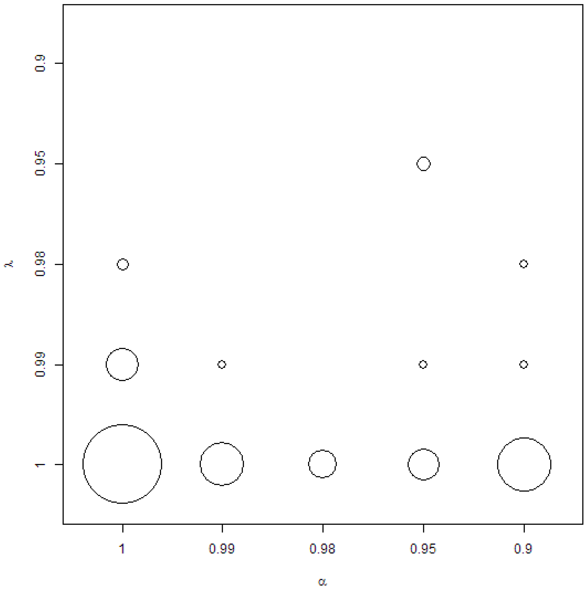
The preferences of forgetting factors can be visualised on a bubble plot in Figure 1. Clearly, it can be seen that, in the case of DMA, DMS and MED models, is preferred if minimising RMSE is the aim. In many cases, is also preferred, meaning that BMA, BMS or BMED is preferred. However, in many cases, remains the preferred option. More discussion about this result is postponed for the end of this section.
The next observation is that the model minimising RMSE was the one with the AR(1) term added in 75% cases if the DMA type was considered. For DMS models, it was 62%, for MED—68%, and for TVP—71%. This means that, in the majority of cases, it is desirable to add an autoregressive term; however, in a reasonable number of cases, it is not.
EWMA (Exponentially Weighted Moving Average) variance updating method was present only in 20% of DMA models which had the smallest RMSE. In the case of DMS models, it was 35%, for MED models—38%, and for TVP models—35%. This suggests that, if minimising errors is the aim, then considering EWMA method is not desirable, and one can stick to the recursive moment estimation (which was proposed in the original paper introducing the DMA method [4]).
Anyway, the idea behind the EWMA method is to erase the possible ARCH effect in residuals. Performing LM–ARCH test with a 5% significance level indicated that the selected models do not have ARCH effects in residuals in 35% of cases of DMA type models, 32% of DMS type models, 33% of MED type models and 28% of TVP type models. Fortunately, as explained in the previous section, the considered Bayesian model combination schemes are recursively updating the error term in equations, so this is not an important obstacle in the case of forecasting. It should be stressed that models were chosen due to minimisation of RMSE, and the verification of ARCH effects was done as an additional check. In other words, for the purpose of this research, the model with ARCH effects, but with smaller RMSE was preferred, even if some model did not possess ARCH effects, but would have larger RMSE.
Of course, it is interesting to estimate how often the lack of ARCH effects could be assumed at a 5% significance level, and, simultaneously, the chosen model was the one with the EWMA estimation method. For DMA type, it was in 10% of cases, for DMS—12%, for MED—14%, and for TVP—10%. Therefore, in line with the previous observation, it can be stated that EWMA allowed for erasing ARCH effects efficiently only in 1/3—1/2 cases in which this method was applied.
To sum up the above results, the following is indicated: first, that DMA is an interesting alternative method (if compared with ARIMA or NAIVE models); secondly, that is usually preferred, but , meaning that most gains in forecast accuracy is due to the certain weighting procedure—not time-varying regression coefficients; third, that the EWMA method is not necessarily “better” than the recursive moment estimation; fourth, that adding the autoregressive term usually (but not always) leads to smaller forecast errors.
5.2. Main Results
Table 4 presents the main outcomes for various model combination schemes. In other words, Table 4 reports the normalized RMSE (nRMSE) from all estimated model. As each type of model was estimated in various versions, in Table 4, the outcomes are present for the one which minimised RMSE for the given type of a model (i.e., out of DMA type models, out of DMS type models, etc.). The normalization of RMSE is done simply by dividing by the mean value of the forecasted time-series. It can be seen (Table 2) that the orders of magnitudes of forecasted commodity prices are quite different. It is easy to switch between RMSE and normalized RMSE having the information from Table 2 and Table 4. However, normalized values seem easier for interpreting the forecasting benefit of each of the models.
Generally, the normalized RMSE is around 0.07. This means that quite accurate forecasts can be produced. In a few cases, very small errors were produced (0.01) or very high errors were produced (0.19). However, for the given commodity, the errors from different models do not differ much.
More information can be derived from Table 5, which presents the results of the Diebold–Mariano tests. The first columns of this table are devoted to comparison of the accuracies of forecasts generated by the DMA method and the NAIVE and the ARIMA models. As a reminder, the null hypothesis of the test is that both forecasts have the same accuracy. For each of the commodities, whether DMA produced smaller RMSE than the NAIVE, and whether it produced smaller RMSE than the ARIMA, was checked. If so, then the alternative hypothesis for the test was taken that the DMA forecast is more accurate than the one from the NAIVE (or from the ARIMA). Otherwise, the NAIVE forecast (or the ARIMA forecast) is more accurate. Clearly, it can be seen that, in the majority of cases, there is a strong evidence to treat DMA as a significantly more accurate forecasting method.
The notation X < Y in Table 5 represents the alternative hypothesis for the Diebold–Mariano test, and it should be read: “The forecast generated by model X is more accurate than the forecast generated by model Y”. Similarly, the notation X > Y should be read: “The forecast generated by model Y is more accurate than the forecast generated by model X”.
Finally, the last two columns in Table 5 are devoted to choosing the “best” model out of all considered ones, for the given commodity price. The “best” model is understood to be the one that generated the smallest RMSE. Next, as already mentioned in the Methodology section, the estimated models were divided into two groups. The first contained DMA, DMS and MED models and the second the TVP, ARIMA and NAIVE. In each group, the representatives with smallest (in the given group) RMSE were chosen. Then, the Diebold–Mariano test was performed to check that, indeed, the forecast generated by one of these representative models is significantly more accurate than the forecasts generated by the second representative model (from another group). The summary of these considerations is presented in Table 6.
Indeed, from Table 6, it can be seen that, in 26% of cases, DMA was the model that generated the smallest RMSE. Moreover, in 22% of cases, it did so and, simultaneously, this result was significant at a 5% significance level according to the described procedure (dividing models into two groups). The DMA model generated the smallest RMSE in 23% of cases. In 13% of cases, it did so, and, simultaneously, this result was significant. The MED model generated the smallest RMSE in 28% of cases. In 17% of cases, it did so, and, simultaneously, this result was significant. It seems worth noticing that the scheme of selecting the model with the highest posterior probability is more popular over the Median Probability Model (MED). The obtained results seem therefore interesting, as they confirm that it is worth putting more attention in practice on the MED combination scheme.
The TVP model generated the smallest RMSE only in 1% of cases. In none of cases did it do so significantly.
BMA, BMS and BMED models were never the ones minimising RMSE out of all considered forecasting models. Together with the already discussed observation from Figure 1, it means that models with are very often minimising RMSE amongst the discussed Bayesian model combination schemes, but they cannot generate significantly more accurate forecasts than the ARIMA or the NAIVE models. On the other hand, if the Bayesian model combination scheme generated such a significantly more accurate forecast, then it was the model with or . Again, looking at Figure 1, it can be expected that this was rather due to than to .
Finally, the NAIVE model generated the smallest RMSE in only 6% of cases. In none of cases did it do so significantly. The ARIMA model generated the smallest RMSE in 16% of cases. In only 4% of cases did it do so, and, simultaneously, this result was significant.
It can be concluded that the considered Bayesian model combination schemes can result in significantly more accurate forecasts. Secondly, both model averaging (like in DMA), and model selection (like in DMS and MED) are efficient methods. It should be stressed that, due to Equation (1) and the way the weights are updated recursively, the forgetting factor plays an important role also in model selection schemes. Its role is connected with the way that the past information is treated. Roughly speaking, the information (how the model behaved) from i periods back is given weight [7,10].
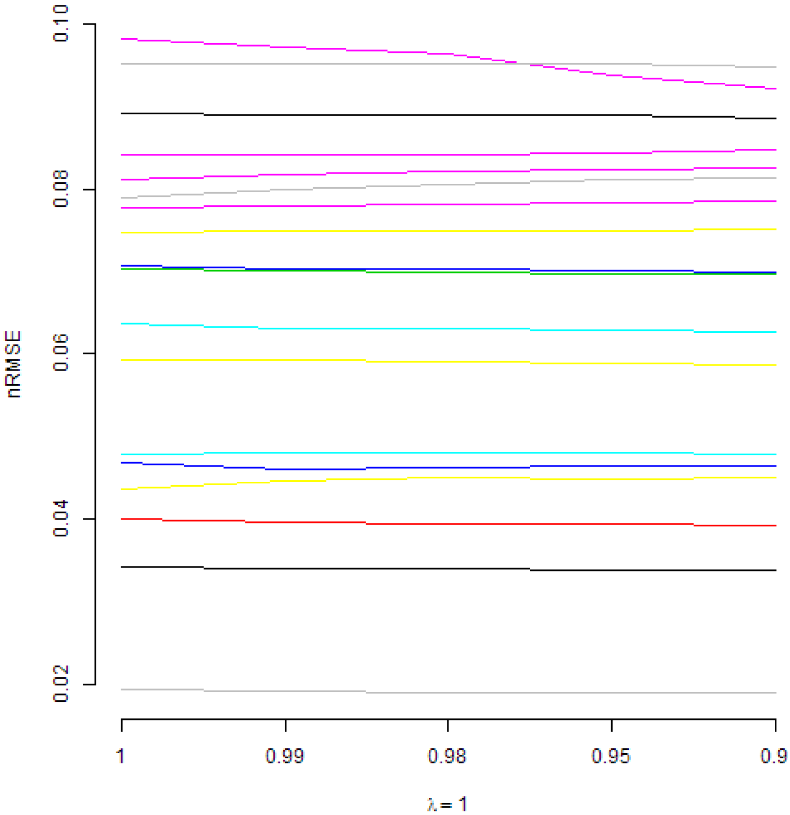
Those figures present normalized RMSE from DMA models with an AR(1) term and with recursive moment estimation used for variance updating. In Figure 2, various are considered. It can be seen that, under such a restriction, higher values of forgetting factors are preferred. A similar conclusion is valid if is fixed and is changing, as it can be seen in Figure 3. However, in Figure 4, it can be seen that, if is fixed, in most cases, changing the value of does not lead to important changes of normalized RMSE. Anyway, in a few cases, the smaller values of are preferred.
5.3. Further Remarks
By looking at rows in Table 4, it could be seen that the average gain in lowering normalized RMSE by applying some of the Bayesian model combination scheme over TVP, ARIMA or NAIVE models is 0.002, which is very small. On the other hand, from Table 5, it was seen that Bayesian model combination schemes very often produce significantly more accurate forecasts, so this gain is important.
It is also interesting to come back to Figure 1 and discussion about the preferred forgetting factors. Usually, if considerations are narrowed just to DMA, DMS and MED models, then the combination of minimises errors. However, when considerations are narrowed to those of DMA, DMS and MED models, which generate significantly more accurate forecasts than TVP, ARIMA and NAIVE, then is preferred, but . Therefore, it is interesting to analyse whether the difference between these two types of models is statistically significant. For this, DMA models with AR(1) term and based on recursive moment estimation for variance updating were compared—in other words, those models with (BMA) with and (DMA). At the 5% significance level, according to the Diebold–Mariano test, DMA generated a more accurate forecast than BMA in 14% of cases, at a 10% significance level—in 23% of cases.
Actually, in Figure 1, some interesting patterns can also be seen for fixed . From the interpretative point of view, the combination is also quite natural. Therefore, Figure 2, Figure 3 and Figure 4 present normalized RMSE for all analysed commodities prices with different combinations of forgetting factors and .
6. Conclusions
It was found that, in general, the Bayesian model combination schemes like Dynamic Model Averaging (DMA), Dynamic Model Selection (DMS) and Median Probability Model (MED) in most of the cases produced significantly more accurate forecasts than the ARIMA, NAIVE or TVP (Time-Varying Parameters regression) models. Interestingly, the MED model in many cases generated smaller RMSE (Root Mean Squared Error) than DMS.
It was found that, indeed, the schemes based on recursive estimation like in DMA, allowing for time-varying regression coefficients and time-varying models’ weights, resulted in smaller RMSE and more accurate forecasts. However, the more thorough analysis suggested that the forecasting benefit from this approach is rather due to time-varying weights, not time-varying regression coefficients. From the economic point of view, this might be interpreted that, in different periods, it is rather the model itself (the collection of predictors) which really matters as opposed to the strength of the relationship between predictors and the given commodity price, which should be modeled more carefully.
Indeed, all considered modeling schemes used in this research were based on the recursive estimations. In other words, forecast at time t was based only on the information available up to the time . Additionally, all information available up to time was used, so, as the new information become available, it was used to update the model’s parameters.
On the other hand, in a numerical sense, the decline in RMSE due to the use of the applied schemes was not very high. Anyway, according to the Diebold–Mariano (DM) test, the applied schemes generated significantly more accurate forecasts.
This research was not based on some index as a proxy of commodities prices. Instead, 69 individual time-series were modeled. Generally, it was confirmed that adding the autoregressive first lag as a predictor improves the forecast accuracy. The advantage of Exponentially Weighted Moving Average (EWMA) in variance updating over the originally proposed recursive moment estimation was not confirmed.
Summarizing the outcomes, the considered Bayesian model combination schemes were found useful, i.e., generating more accurate forecasts in most of the cases.
Funding
The research was funded by the Polish National Science Centre grant under the contract number DEC-2015/19/N/HS4/00205.
Conflicts of Interest
The authors declare no conflict of interest. The founding sponsors had no role in the design of the study; in the collection, analyses, or interpretation of data; in the writing of the manuscript, and in the decision to publish the results.
Abbreviations
The following abbreviations are used in this manuscript:
| ARIMA | Auto ARIMA model described by Hyndman and Khandakar [71] |
| BMA | Bayesian Model Averaging as a special case of DMA with forgetting factors |
| BMED | Bayesian Median Probability Model as a special case of MED with forgetting factors |
| BMS | Bayesian Model Selection as a special case of DMS with forgetting factors |
| DM | The Diebold–Mariano test [75] |
| DMA | Dynamic Model Averaging proposed by Raftery et al. [4] |
| DMS | Dynamic Model Selection, i.e., model averaging in DMA replaced by selecting the model with the highest posterior probability |
| MED | Median Probability Model of Barbieri and Berger [74] |
| NAIVE | the naive forecast, i.e., the last observation is the one-ahead forecast |
| RMSE | Root Mean Squared Error |
| nRMSE | Normalized RMSE, i.e., RMSE divided by the mean value of the forecasted time-series |
| TVP | Time-Varying Parameters, i.e., DMA reduced to exactly one model, i.e., the one with all predictors |
References
- Arouri, M.E.H.; Dinh, T.H.; Nguyen, D.K. Time-varying Predictability in Crude-oil Markets: The Case of GCC Countries. Energy Policy 2010, 38, 4371–4380. [Google Scholar] [CrossRef]
- Henkel, S.J.; Martin, J.S.; Nardari, F. Time-varying Short-horizon Predictability. J. Financ. Econ. 2011, 99, 560–580. [Google Scholar] [CrossRef]
- Rapach, D.; Strauss, J.; Zhou, G. International Stock Return Predictability: What Is the Role of the United States? J. Finance 2013, 68, 1633–1662. [Google Scholar] [CrossRef] [Green Version]
- Raftery, A.; Kárný, M.; Ettler, P. Online Prediction under Model Uncertainty via Dynamic Model Averaging: Application to a Cold Rolling Mill. Technometrics 2010, 52, 52–66. [Google Scholar] [CrossRef] [PubMed]
- The World Bank. Commodity Price Data; The World Bank: Washington, DC, USA, 2017. [Google Scholar]
- Gargano, A.; Timmermann, A. Forecasting Commodity Price Indexes Using Macroeconomic and Financial Predictors. Int. J. Forecast. 2014, 30, 825–843. [Google Scholar] [CrossRef]
- Buncic, D.; Moretto, C. Forecasting Copper Prices with Dynamic Averaging and Selection Models. N. Am. J. Econ. Finance 2015, 33, 1–38. [Google Scholar] [CrossRef]
- Drachal, K. Forecasting Spot Oil Price in a Dynamic Model Averaging Framework—Have the Determinants Changed over Time? Energy Econ. 2016, 60, 35–46. [Google Scholar] [CrossRef]
- Risse, M.; Kern, M. Forecasting House-price Growth in the Euro Area with Dynamic Model Averaging. N. Am. J. Econ. Finance 2016, 38, 70–85. [Google Scholar] [CrossRef]
- Baur, D.; Beckmann, J.; Czudaj, R. A Melting Pot-Gold Price Forecasts under Model and Parameter Uncertainty. Int. Rev. Financ. Anal. 2016, 48, 282–291. [Google Scholar] [CrossRef]
- Naser, H. Estimating and Forecasting the Real Prices of Crude Oil: A Data Rich Model Using a Dynamic Model Averaging (DMA) Approach. Energy Econ. 2016, 56, 75–87. [Google Scholar] [CrossRef]
- Wei, Y.; Cao, Y. Forecasting House Prices Using Dynamic Model Averaging Approach: Evidence from China. Econ. Model. 2017, 61, 147–155. [Google Scholar] [CrossRef]
- Aye, G.; Gupta, R.; Hammoudeh, S.; Kim, W. Forecasting the Price of Gold Using Dynamic Model Averaging. Int. Rev. Financ. Anal. 2015, 41, 257–266. [Google Scholar] [CrossRef]
- Risse, M.; Ohl, L. Using Dynamic Model Averaging in State Space Representation with Dynamic Occam’s Window and Applications to the Stock and Gold Market. J. Empir. Finance 2017, 44, 158–176. [Google Scholar] [CrossRef]
- Onorante, L.; Raftery, A. Dynamic Model Averaging in Large Model Spaces Using Dynamic Occam’s Window. Eur. Econ. Rev. 2016, 81, 2–14. [Google Scholar] [CrossRef] [PubMed]
- Baxa, J.; Plašil, M.; Vašiček, B. Inflation and the Steeplechase between Economic Activity Variables: Evidence for G7 Countries. B.E. J. Macroecon. 2017, 17, 42. [Google Scholar] [CrossRef]
- Del Negro, M.; Hasegawa, R.; Schorfheide, F. Dynamic Prediction Pools: An Investigation of Financial Frictions and Forecasting Performance. J. Econom. 2016, 192, 391–405. [Google Scholar] [CrossRef]
- Di Filippo, G. Dynamic Model Averaging and CPI Inflation Forecasts: A Comparison between the Euro Area and the United States. J. Forecast. 2015, 34, 619–648. [Google Scholar] [CrossRef]
- Ferreira, D.; Palma, A. Forecasting Inflation with the Phillips Curve: A Dynamic Model Averaging Approach for Brazil. Rev. Bras. Econ. 2015, 69, 451–465. [Google Scholar] [CrossRef]
- Koop, G.; Korobilis, D. Forecasting Inflation Using Dynamic Model Averaging. Int. Econ. Rev. 2012, 53, 867–886. [Google Scholar] [CrossRef]
- Koop, G.; Korobilis, D. UK Macroeconomic Forecasting with Many Predictors: Which Models Forecast Best and When Do They Do So? Econ. Model. 2011, 28, 2307–2318. [Google Scholar] [CrossRef]
- Koop, G.; Korobilis, D. A New Index of Financial Conditions. Eur. Econ. Rev. 2014, 71, 101–116. [Google Scholar] [CrossRef] [Green Version]
- Bork, L.; Moller, S. Forecasting House Prices in the 50 States Using Dynamic Model Averaging and Dynamic Model Selection. Int. J. Forecast. 2015, 31, 63–78. [Google Scholar] [CrossRef]
- De Bruyn, R.; Gupta, R.; Van Eyden, R. Can We Beat the Random-walk Model for the South African Rand—U.S. Dollar and South African Rand—UK Pound Exchange Rates? Evidence from Dynamic Model Averaging. Emerg. Mark. Finance Trade 2015, 51, 502–524. [Google Scholar] [CrossRef]
- Gupta, R.; Hammoudeh, S.; Kim, W.; Simo-Kengne, B. Forecasting China’s Foreign Exchange Reserves Using Dynamic Model Averaging: The Roles of Macroeconomic Fundamentals, Financial Stress and Economic Uncertainty. N. Am. J. Econ. Finance 2014, 28, 170–189. [Google Scholar] [CrossRef]
- Koop, G.; Tole, L. Forecasting the European Carbon Market. J. R. Stat. Soc. Ser. A Stat. Soc. 2013, 176, 723–741. [Google Scholar] [CrossRef]
- Liu, J.; Wei, Y.; Ma, F.; Wahab, M. Forecasting the Realized Range-based Volatility Using Dynamic Model Averaging Approach. Econ. Model. 2017, 61, 12–26. [Google Scholar] [CrossRef]
- Wang, Y.; Ma, F.; Wei, Y.; Wu, C. Forecasting Realized Volatility in a Changing World: A Dynamic Model Averaging Approach. J. Bank. Finance 2016, 64, 136–149. [Google Scholar] [CrossRef]
- Naser, H.; Alaali, F. Can Oil Prices Help Predict US Stock Market Returns? Evidence Using a Dynamic Model Averaging (DMA) Approach. Empir. Econ. 2017. [Google Scholar] [CrossRef]
- Bates, J.; Granger, C. The Combination of Forecasts. Oper. Res. Q. 1969, 20, 451–468. [Google Scholar] [CrossRef]
- Baumeister, C.; Kilian, L. Forecasting the Real Price of Oil in a Changing World: A Forecast Combination Approach. J. Bus. Econ. Stat. 2015, 33, 338–351. [Google Scholar] [CrossRef]
- Kaya, H. Forecasting the Price of Crude Oil with Multiple Predictors. Siyasal Bilgiler Fakültesi Dergisi (İSMUS) 2016, 1, 133–151. [Google Scholar]
- Wang, Y.; Liu, L.; Wu, C. Forecasting the Real Prices of Crude Oil Using Forecast Combinations over Time-varying Parameter Models. Energy Econ. 2017, 66, 337–348. [Google Scholar] [CrossRef]
- Moral-Benito, E. Model Averaging in Economics: An Overview. J. Econ. Surv. 2015, 29, 46–75. [Google Scholar] [CrossRef]
- Steel, M. Model Averaging and its Use in Economics. arXiv, 2017; arXiv:1709.08221. [Google Scholar]
- Greenberg, E. Introduction to Bayesian Econometrics; Cambridge University Press: Cambridge, UK, 2012. [Google Scholar]
- Koop, G. Bayesian Methods for Empirical Macroeconomics with Big Data. Rev. Econ. Anal. 2017, 9, 33–56. [Google Scholar]
- Lee, C.Y.; Huh, S.Y. Forecasting Long-term Crude Oil Prices Using a Bayesian Model with Informative Priors. Sustainability 2017, 9, 190. [Google Scholar] [CrossRef]
- Yin, X.; Peng, J.; Tang, T. Improving the Forecasting Accuracy of Crude Oil Prices. Sustainability 2018, 10, 454. [Google Scholar] [CrossRef]
- Kriechbaumer, T.; Angus, A.; Parsons, D.; Rivas Casado, M. An Improved Wavelet-ARIMA Approach for Forecasting Metal Prices. Resour. Policy 2014, 39, 32–41. [Google Scholar] [CrossRef] [Green Version]
- Wang, Q.; Sun, X. Crude Oil Price: Demand, Supply, Economic Activity, Economic Policy Uncertainty and Wars—From the Perspective of Structural Equation Modelling (SEM). Energy 2017, 133, 483–490. [Google Scholar] [CrossRef]
- Cross, J.; Nguyen, B. The Relationship between Global Oil Price Shocks and China’s Output: A Time-varying Analysis. Energy Econ. 2017, 62, 79–91. [Google Scholar] [CrossRef]
- Gangopadhyay, K.; Jangir, A.; Sensarma, R. Forecasting the Price of Gold: An Error Correction Approach. IIMB Manag. Rev. 2016, 28, 6–12. [Google Scholar] [CrossRef]
- Gil-Alana, L.; Chang, S.; Balcilar, M.; Aye, G.; Gupta, R. Persistence of Precious Metal Prices: A Fractional Integration Approach with Structural Breaks. Resour. Policy 2015, 44, 57–64. [Google Scholar] [CrossRef]
- Kim, J.M.; Jung, H. Time Series Forecasting Using Functional Partial Least Square Regression with Stochastic Volatility, GARCH, and Exponential Smoothing. J. Forecast. 2017, 37, 269–280. [Google Scholar] [CrossRef]
- Hamdi, M.; Aloui, C. Forecasting Crude Oil Price Using Artificial Neural Networks: A Literature Survey. Econ. Bull. 2015, 35, 1339–1359. [Google Scholar]
- Liu, C.; Hu, Z.; Li, Y.; Liu, S. Forecasting Copper Prices by Decision Tree Learning. Resour. Policy 2017, 52, 427–434. [Google Scholar] [CrossRef]
- Zhao, Y.; Li, J.; Yu, L. A Deep Learning Ensemble Approach for Crude Oil Price Forecasting. Energy Econ. 2017, 66, 9–16. [Google Scholar] [CrossRef]
- Welch, I.; Goyal, A. A Comprehensive Look at The Empirical Performance of Equity Premium Prediction. Rev. Financ. Stud. 2008, 21, 1455–1508. [Google Scholar] [CrossRef]
- Ghalayini, L. Modeling and Forecasting Spot Oil Price. Eurasian Bus. Rev. 2017, 7, 355–373. [Google Scholar] [CrossRef]
- Tan, X.; Ma, Y. The Impact of Macroeconomic Uncertainty on International Commodity Prices: Empirical Analysis Based on TVAR Model. China Finance Rev. Int. 2017, 7, 163–184. [Google Scholar] [CrossRef]
- Kagraoka, Y. Common Dynamic Factors in Driving Commodity Prices: Implications of a Generalized Dynamic Factor Model. Econ. Model. 2016, 52, 609–617. [Google Scholar] [CrossRef]
- Lübbers, J.; Posch, P. Commodities’ Common Factor: An Empirical Assessment of the Markets’ Drivers. J. Commod. Market. 2016, 4, 28–40. [Google Scholar] [CrossRef]
- Arango, L.; Arias, F.; Florez, A. Determinants of Commodity Prices. Appl. Econ. 2012, 44, 135–145. [Google Scholar] [CrossRef]
- Byrne, J.; Fazio, G.; Fiess, N. Primary Commodity Prices: Co-movements, Common Factors and Fundamentals. J. Dev. Econ. 2013, 101, 16–26. [Google Scholar] [CrossRef]
- Alam, M.; Gilbert, S. Monetary Policy Shocks and the Dynamics of Agricultural Commodity Prices: Evidence from Structural and Factor-Augmented VAR Analyses. Agric. Econ. 2017, 48, 15–27. [Google Scholar] [CrossRef]
- Chen, Y.; Rogoff, K.; Rossi, B. Can Exchange Rates Forecast Commodity Prices? Q. J. Econ. 2010, 125, 1145–1194. [Google Scholar] [CrossRef]
- Arslan-Ayaydin, O.; Khagleeva, I. Chapter: The Dynamics of Crude Oil Spot and Futures Markets. In Energy Economics and Financial Markets; Springer: Berlin, Germany, 2013; pp. 159–173. [Google Scholar]
- Hong, H.; Yogo, M. What does Futures Market Interest Tell Us about the Macroeconomy and Asset Prices? J. Financ. Econ. 2012, 105, 473–490. [Google Scholar] [CrossRef]
- Chen, S.S. Commodity Prices and Related Equity Prices. Can. J. Econ. 2016, 49, 949–967. [Google Scholar] [CrossRef]
- Wang, Y.; Liu, L.; Diao, X.; Wu, C. Forecasting the Real Prices of Crude Oil under Economic and Statistical Constraints. Energy Econ. 2015, 51, 599–608. [Google Scholar] [CrossRef]
- Schiller, R. Online Data Robert Shiller. 2017. Available online: http://www.econ.yale.edu/~shiller/data.htm (accessed on 12 March 2018).
- FRED. Economic Data. Federal Reserve Bank of St. Louis Web Site, 2017. Available online: https://fred.stlouisfed.org (accessed on 12 March 2018).
- Kilian, L. Updated Version of the Index of Global Real Economic Activity in Industrial Commodity Markets. The University of Michigan Web Site. Available online: http://www-personal.umich.edu/~lkilian/reaupdate.txt (accessed on 12 March 2018).
- U.S. Commodity Futures Trading Commission. Historical Compressed. 2017; Commodity Futures Trading Commission Web Site. Available online: http://www.cftc.gov/MarketReports/CommitmentsofTraders/HistoricalCompressed/index.htm (accessed on 12 March 2018).
- Yogo, M. Research. Motohiro Yogo Web Site, 2017. Available online: http://sites.google.com/site/motohiroyogo (accessed on 12 March 2018).
- Thomson Reuters. Commodity Indices. Financial Thomson Reuters Web Site, 2017. Available online: http://financial.thomsonreuters.com/en/products/data-analytics/market-data/indices/commodity-index.html (accessed on 12 March 2018).
- Drachal, K. Comparison between Bayesian and Information-theoretic Model Averaging: Fossil Fuels Prices Example. Energy Econ. 2018, 74, 208–251. [Google Scholar] [CrossRef]
- R Core Team. R: A Language and Environment for Statistical Computing; R Foundation for Statistical Computing: Vienna, Austria, 2013. [Google Scholar]
- Drachal, K. fDMA: Dynamic Model Averaging and Dynamic Model Selection for Continuous Outcomes. R Package Documentation Web Site, 2017. Available online: https://CRAN.R-project.org/package=fDMA (accessed on 12 March 2018).
- Hyndman, R.; Khandakar, Y. Automatic Time Series Forecasting: The forecast Package for R. J. Stat. Softw. 2008, 26, 1–22. [Google Scholar]
- Belmonte, M.; Koop, G. Model Switching and Model Averaging in Time-varying Parameter Regression Models. Adv. Econ. 2014, 34, 45–69. [Google Scholar]
- Drachal, K. Determining Time-varying Drivers of Spot Oil Price in a Dynamic Model Averaging Framework. Energies 2018, 11, 1207. [Google Scholar] [CrossRef]
- Barbieri, M.; Berger, J. Optimal Predictive Model Selection. Ann. Stat. 2004, 32, 870–897. [Google Scholar]
- Diebold, F.; Mariano, R. Comparing Predictive Accuracy. J. Bus. Econ. Stat. 1995, 13, 253–263. [Google Scholar] [Green Version]
- Bergmeir, C.; Hyndman, R.; Koo, B. A Note on the Validity of Cross-validation for Evaluating Autoregressive Time Series Prediction. Comput. Stat. Data Anal. 2018, 120, 70–83. [Google Scholar] [CrossRef]
Figure 1.
Combination of forgetting factors for DMA, DMS and MED models, which minimise RMSE. Circles are proportional to the number of models.
Figure 1.
Combination of forgetting factors for DMA, DMS and MED models, which minimise RMSE. Circles are proportional to the number of models.

Figure 2.
Normalized RMSE for all commodities vs. different values of forgetting factors.
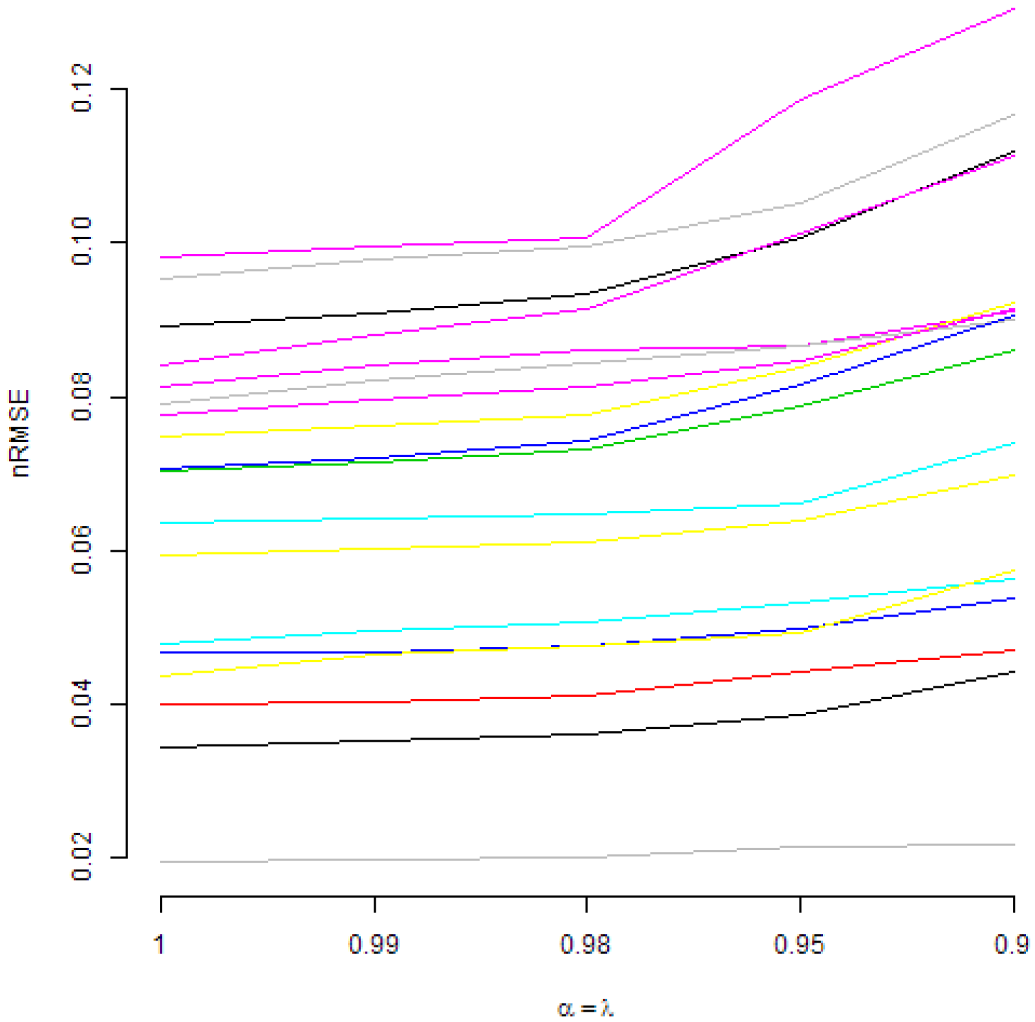
Figure 3.
Normalized RMSE for all commodities vs. different values of forgetting factors.
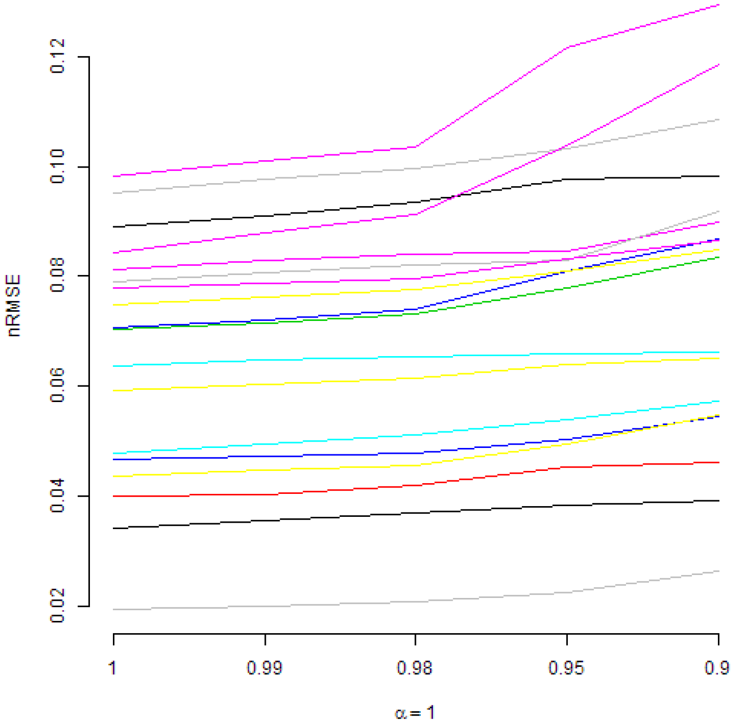
Figure 4.
Normalized RMSE for all commodities vs. different values of forgetting factors.


Table 1.
Commodities abbreviations. Details can be found in the original source: The World Bank [5].
Table 1.
Commodities abbreviations. Details can be found in the original source: The World Bank [5].
| IBEVERAGES | Beverages index includes cocoa, coffee and tea. |
|---|---|
| IFOOD | Food index includes fats and oils, grains and other food items. |
| IFATS_OILS | Fats and oils index includes coconut oil, groundnut oil, palm oil, soybeans, soybean oil and soybean meal. |
| IGRAINS | Grains index includes barley, maize, rice and wheat. |
| IOTHERFOOD | Other food index includes bananas, beef, chicken meat, oranges and sugar. |
| IRAW_MATERIAL | Agricultural raw materials index includes timber and other raw materials. |
| ITIMBER | Timber index includes tropical hard logs and sawn wood. |
| IOTHERRAWMAT | Other raw materials index includes cotton, natural rubber and tobacco. |
| IAGRICULTURE | Agriculture index includes beverages, food and agricultural raw materials. |
| ALUMINUM | Aluminium (LME) London Metal Exchange, unalloyed primary ingots, high grade, minimum 99.7% purity, settlement price beginning 2005; previously cash price |
| BANANA_US | Bananas (Central & South America), major brands, US import price, free on truck US (f.o.t.) Gulf ports |
| BARLEY | Barley (Canada), feed, Western No. 1, Winnipeg Commodity Exchange, spot, wholesale farmers’ price |
| COAL_AUS | Coal (Australia), thermal, f.o.b. piers, Newcastle/Port Kembla, 6300 kcal/kg (11,340 btu/lb), less than 0.8%, sulfur 13% ash beginning January 2002; previously 6667 kcal/kg (12,000 btu/lb), less than 1.0% sulfur, 14% ash |
| COCOA | Cocoa (ICCO), International Cocoa Organization daily price, average of the first three positions on the terminal markets of New York and London, nearest three future trading months. |
| COCONUT_OIL | Coconut oil (Philippines/Indonesia), bulk, c.i.f. Rotterdam |
| COFFEE_ARABIC | Coffee (ICO), International Coffee Organization indicator price, other mild Arabicas, average New York and Bremen/Hamburg markets, ex-dock |
| COFFEE_ROBUS | Coffee (ICO), International Coffee Organization indicator price, Robustas, average New York and Le Havre/Marseilles markets, ex-dock |
| COPPER | Copper (LME), grade A, minimum 99.9935% purity, cathodes and wire bar shapes, settlement price |
| COPRA | Copra (Philippines/Indonesia), bulk, c.i.f. N.W. Europe |
| COTTON_A_INDX | Cotton (Cotton Outlook “CotlookA index”), middling 1-3/32 inch, traded in Far East, C/F beginning 2006; previously Northern Europe, c.i.f. |
| CRUDE_PETRO | Crude oil, average spot price of Brent, Dubai and West Texas Intermediate, equally weighed |
| CRUDE_BRENT | Crude oil, U.K. Brent 38’ API, f.o.b. U.K ports, spot price |
| CRUDE_DUBAI | Crude oil, Dubai Fateh 32’ API, f.o.b. Dubai, spot price |
| CRUDE_WTI | Crude oil, West Texas Intermediate (WTI) 40’ API, f.o.b. Midland Texas, spot price |
| DAP | DAP (diammonium phosphate), standard size, bulk, spot, f.o.b. US Gulf |
| IENERGY | Energy index, a Laspeyres Index with fixed weights based on 2002–2004 average developing countries export values, for coal, crude oil and natural gas. |
| IFERTILIZERS | Fertilizers index includes natural phosphate rock, phosphate, potassium and nitrogenous products. |
| FISH_MEAL | Fishmeal (any origin), 64–65%, c&f Bremen, estimates based on wholesale price, beginning 2004; previously c&f Hamburg |
| GOLD | Gold (UK), 99.5% fine, London afternoon fixing, average of daily rates |
| GRNUT_OIL | Groundnut oil (any origin), c.i.f. Rotterdam |
| LEAD | Lead (LME), refined, 99.97% purity, settlement price |
| LOGS_CMR | Logs (West Africa), sapele, high quality (loyal and marchand), 80 centimeter or more, f.o.b. Douala, Cameroon beginning January 1996; previously of unspecified dimension |
| LOGS_MYS | Logs (Malaysia), meranti, Sarawak, sale price charged by importers, Tokyo beginning February 1993; previously average of Sabah and Sarawak weighted by Japanese import volumes |
| MAIZE | Maize (US), no. 2, yellow, f.o.b. US Gulf ports |
| BEEF | Meat, beef (Australia/New Zealand), chucks and cow forequarters, frozen boneless, 85% chemical lean, c.i.f. U.S. port (East Coast), ex-dock, beginning November 2002; previously cow forequarters |
| CHICKEN | Meat, sheep (New Zealand), frozen whole carcasses Prime Medium (PM) wholesale, Smithfield, London beginning January 2006; previously Prime Light (PL) |
| IMETMIN | Metals and minerals index includes aluminum, copper, iron ore, lead, nickle, tin and zinc. |
| NGAS_US | Natural Gas (U.S.), spot price at Henry Hub, Louisiana |
| NICKEL | Nickel (LME), cathodes, minimum 99.8% purity, settlement price beginning 2005; previously cash price |
| INONFUEL | Non-energy index, a Laspeyres Index with fixed weights based on 2002–2004 average developing countries export values, for 34 commodities contain in the agriculture, fertilizer, and metals and minerals indices. |
| ORANGE | Oranges (Mediterranean exporters) navel, EEC indicative import price, c.i.f. Paris |
| PALM_OIL | Palm oil (Malaysia), 5% bulk, c.i.f. N. W. Europe |
| PLATINUM | Platinum (UK), 99.9% refined, London afternoon fixing |
| PLYWOOD | Plywood (Africa and Southeast Asia), Lauan, 3-ply, extra, 91 cm × 182 cm × 4 mm, wholesale price, spot Tokyo |
| POTASH | Potassium chloride (muriate of potash), standard grade, spot, f.o.b. Vancouver |
| RICE_05 | Rice (Thailand), 5% broken, white rice (WR), milled, indicative price based on weekly surveys of export transactions, government standard, f.o.b. Bangkok |
| RUBBER1_MYSG | Rubber (Asia), RSS3 grade, Singapore Commodity Exchange Ltd. (SICOM) nearby contract beginning 2004; during 2000 to 2003, Singapore RSS1; previously Malaysia RSS1 |
| SAWNWD_MYS | Sawnwood (Malaysia), dark red seraya/meranti, select and better quality, average 7 to 8 inches; length average 12 to 14 inches; thickness 1 to 2 inch(es); kiln dry, c. & f. UK ports, with 5% agents commission including premium for products of certified sustainable forest beginning January 2005; previously excluding the premium |
| SHRIMP_MEX | Shrimp, (Mexico), west coast, frozen, white, No. 1, shell-on, headless, 26 to 30 count per pound, wholesale price at New York |
| SILVER | Silver (Handy & Harman), 99.9% grade refined, New York |
| SORGHUM | Sorghum (US), no. 2 milo yellow, f.o.b. Gulf ports |
| SOYBEAN_MEAL | Soybean meal (any origin), Argentine 45/46% extraction, c.i.f. Rotterdam beginning 1990; previously US 44% |
| SOYBEAN_OIL | Soybean oil (Any origin), crude, f.o.b. ex-mill Netherlands |
| SOYBEANS | Soybeans (US), c.i.f. Rotterdam |
| SUGAR_EU | Sugar (EU), European Union negotiated import price for raw unpackaged sugar from African, Caribbean and Pacific (ACP) under Lome Conventions, c.I.f. European ports |
| SUGAR_US | Sugar (US), nearby futures contract, c.i.f. |
| SUGAR_WLD | Sugar (world), International Sugar Agreement (ISA) daily price, raw, f.o.b. and stowed at greater Caribbean ports |
| TEA_AVG | Tea, average three auctions, arithmetic average of quotations at Kolkata, Colombo and Mombasa/Nairobi. |
| TEA_COLOMBO | Tea (Colombo auctions), Sri Lankan origin, all tea, arithmetic average of weekly quotes. |
| TEA_KOLKATA | Tea (Kolkata auctions), leaf, include excise duty, arithmetic average of weekly quotes. |
| TEA_MOMBASA | Tea (Mombasa/Nairobi auctions), African origin, all tea, arithmetic average of weekly quotes. |
| TIN | Tin (LME), refined, 99.85% purity, settlement price |
| TOBAC_US | Tobacco (any origin), unmanufactured, general import, cif, US |
| TSP | TSP (triple superphosphate), up to September 2006 bulk, spot, f.o.b. US Gulf; from October 2006 onwards Tunisian, granular, f.o.b. |
| UREA_EE_BULK | Urea, (Black Sea), bulk, spot, f.o.b. Black Sea (primarily Yuzhnyy) beginning July 1991; for 1985–1991 (June) f.o.b. Eastern Europe |
| WHEAT_US_HRW | Wheat (US), no. 1, hard red winter, ordinary protein, export price delivered at the US Gulf port for prompt or 30 days shipment |
| WHEAT_US_SRW | Wheat (US), no. 2, soft red winter, export price delivered at the US Gulf port for prompt or 30 days shipment |
| WOODPULP | Woodpulp (Sweden), softwood, sulphate, bleached, air-dry weight, c.i.f. North Sea ports |
| ZINC | Zinc (LME), high grade, minimum 99.95% purity, settlement price beginning April 1990; previously special high grade, minimum 99.995%, cash prices |
Table 2.
Descriptive statistics.
| Variable | Mean | Standard Deviation | Min | Max | Skewness | Kurtosis |
|---|---|---|---|---|---|---|
| dpr | −0.0134 | 0.0035 | −0.0200 | −0.0057 | 0.2356 | −0.8496 |
| str | 0.0358 | 0.0277 | 0.0001 | 0.1047 | 0.2098 | −1.0013 |
| ltr | 0.0553 | 0.0263 | 0.0150 | 0.1356 | 0.5970 | −0.0447 |
| ts | 0.0195 | 0.0107 | −0.0053 | 0.0376 | −0.2611 | −0.9187 |
| drs | 0.0327 | 0.0126 | 0.0036 | 0.0593 | −0.2889 | −0.8796 |
| cpi | 0.0022 | 0.0026 | −0.0179 | 0.0137 | −1.4017 | 11.2535 |
| ip | 0.0017 | 0.0061 | −0.0440 | 0.0203 | −1.5642 | 9.4380 |
| une | 0.0609 | 0.0146 | 0.0380 | 0.1000 | 0.7915 | −0.0500 |
| aud | −0.0004 | 0.0332 | −0.1798 | 0.0885 | −0.7722 | 2.7502 |
| inr | −0.0045 | 0.0186 | −0.1956 | 0.0594 | −3.1422 | 28.1909 |
| kei | −0.0167 | 0.2709 | −1.3324 | 0.6661 | 0.0505 | 1.5030 |
| op | 0.0136 | 0.0224 | −0.0727 | 0.0937 | −0.1124 | 3.4690 |
| tr | 0.0010 | 0.0338 | −0.2010 | 0.1168 | −0.7119 | 4.1604 |
| m | 0.0047 | 0.0083 | −0.0337 | 0.0574 | 1.5217 | 9.2340 |
| IBEVERAGES | −0.0002 | 0.0462 | −0.1592 | 0.2870 | 0.8529 | 4.7751 |
| IFOOD | 0.0009 | 0.0305 | −0.1877 | 0.1500 | −0.1921 | 4.6650 |
| IFATS_OILS | 0.0006 | 0.0459 | −0.2540 | 0.1998 | −0.3230 | 3.6843 |
| IGRAINS | 0.0005 | 0.0415 | −0.1962 | 0.1837 | 0.1331 | 2.2778 |
| IOTHERFOOD | 0.0019 | 0.0336 | −0.1016 | 0.1055 | 0.1153 | 0.3257 |
| IRAW_MATERIAL | 0.0012 | 0.0256 | −0.0901 | 0.1103 | 0.3225 | 2.7758 |
| ITIMBER | 0.0016 | 0.0338 | −0.1317 | 0.2011 | 1.0682 | 7.1127 |
| IOTHERRAWMAT | 0.0007 | 0.0347 | −0.1967 | 0.1147 | −0.5056 | 3.8493 |
| IAGRICULTURE | 0.0008 | 0.0241 | −0.1591 | 0.0941 | −0.4836 | 5.1574 |
| ALUMINUM | 0.0008 | 0.0561 | −0.3262 | 0.1801 | −0.5625 | 3.6371 |
| BANANA_US | 0.0028 | 0.1619 | −0.4556 | 0.5934 | 0.3911 | 1.5758 |
| BARLEY | 0.0015 | 0.0680 | −0.2788 | 0.2832 | −0.0479 | 2.5754 |
| COAL_AUS | 0.0030 | 0.0558 | −0.3285 | 0.3637 | 0.2609 | 8.5692 |
| COCOA | −0.0005 | 0.0569 | −0.1948 | 0.2309 | 0.0823 | 0.8005 |
| COCONUT_OIL | 0.0010 | 0.0782 | −0.2598 | 0.3512 | 0.3355 | 1.2619 |
| COFFEE_ARABIC | −0.0001 | 0.0756 | −0.3525 | 0.4227 | 0.6971 | 4.0604 |
| COFFEE_ROBUS | −0.0007 | 0.0673 | −0.2498 | 0.3779 | 0.6395 | 3.4206 |
| COPPER | 0.0039 | 0.0635 | −0.3501 | 0.2492 | −0.3496 | 4.1479 |
| COPRA | 0.0010 | 0.0760 | −0.2128 | 0.3258 | 0.3644 | 1.3311 |
| COTTON_A_INDX | −0.0003 | 0.0560 | −0.2690 | 0.2006 | −0.0479 | 2.7694 |
| CRUDE_PETRO | 0.0016 | 0.0874 | −0.4388 | 0.4304 | −0.4109 | 3.7925 |
| CRUDE_BRENT | 0.0017 | 0.0910 | −0.3834 | 0.4326 | −0.2648 | 2.7104 |
| CRUDE_DUBAI | 0.0017 | 0.0928 | −0.5401 | 0.4910 | −0.5290 | 6.1827 |
| CRUDE_WTI | 0.0014 | 0.0851 | −0.3968 | 0.3755 | −0.4118 | 2.7034 |
| DAP | 0.0012 | 0.0619 | −0.4597 | 0.2551 | −0.9681 | 12.9591 |
| IENERGY | 0.0015 | 0.0720 | −0.3337 | 0.3449 | −0.4010 | 2.8708 |
| IFERTILIZERS | 0.0020 | 0.0461 | −0.2749 | 0.2425 | −0.3816 | 5.6836 |
| FISH_MEAL | 0.0026 | 0.0433 | −0.1542 | 0.2002 | 0.2202 | 1.3521 |
| GOLD | 0.0029 | 0.0356 | −0.1248 | 0.1601 | 0.3494 | 1.3229 |
| GRNUT_OIL | 0.0012 | 0.0515 | −0.2102 | 0.2607 | 0.3673 | 3.9632 |
| LEAD | 0.0045 | 0.0702 | −0.2933 | 0.3091 | −0.3071 | 2.6723 |
| LOGS_CMR | 0.0021 | 0.0345 | −0.1743 | 0.1440 | −0.2417 | 3.5366 |
| LOGS_MYS | 0.0013 | 0.0500 | −0.1931 | 0.2941 | 0.8165 | 5.0984 |
| MAIZE | 0.0001 | 0.0586 | −0.2448 | 0.2975 | −0.1347 | 3.5803 |
| BEEF | 0.0015 | 0.0395 | −0.1780 | 0.1432 | −0.1629 | 2.4215 |
| CHICKEN | 0.0026 | 0.0205 | −0.0558 | 0.1045 | 0.8058 | 3.0832 |
| IMETMIN | 0.0021 | 0.0496 | −0.3045 | 0.1585 | −0.8080 | 5.0908 |
| NGAS_US | 0.0002 | 0.1241 | −0.4055 | 0.4779 | 0.0691 | 1.6753 |
| NICKEL | 0.0022 | 0.0856 | −0.3824 | 0.5811 | 0.7231 | 5.7015 |
| INONFUEL | 0.0012 | 0.0265 | −0.2032 | 0.1002 | −1.1311 | 9.2270 |
| ORANGE | 0.0022 | 0.1233 | −0.4199 | 0.4127 | −0.2108 | 1.0353 |
| PALM_OIL | 0.0001 | 0.0739 | −0.3469 | 0.2731 | −0.3735 | 2.4278 |
| PLATINUM | 0.0021 | 0.0527 | −0.2929 | 0.2335 | −0.4484 | 4.7605 |
| PLYWOOD | 0.0019 | 0.0393 | −0.1583 | 0.1781 | 0.8362 | 4.3207 |
| POTASH | 0.0025 | 0.0403 | −0.4158 | 0.3438 | −1.0375 | 41.9405 |
| RICE_05 | 0.0011 | 0.0580 | −0.2424 | 0.4233 | 1.2896 | 8.8429 |
| RUBBER1_MYSG | 0.0009 | 0.0708 | −0.3904 | 0.2121 | −0.4335 | 3.1845 |
| SAWNWD_MYS | 0.0018 | 0.0346 | −0.1401 | 0.2382 | 1.1335 | 10.5032 |
| SHRIMP_MEX | −0.0001 | 0.0424 | −0.2432 | 0.1839 | −0.6345 | 7.0185 |
| SILVER | 0.0015 | 0.0621 | −0.2143 | 0.2604 | 0.1165 | 1.6884 |
| SORGHUM | 0.0006 | 0.0634 | −0.2777 | 0.3419 | −0.0446 | 3.8254 |
| SOYBEAN_MEAL | 0.0008 | 0.0567 | −0.1858 | 0.2176 | 0.2146 | 1.6060 |
| SOYBEAN_OIL | 0.0007 | 0.0557 | −0.2785 | 0.2611 | −0.0453 | 3.2895 |
| SOYBEANS | 0.0006 | 0.0503 | −0.2561 | 0.2140 | −0.2455 | 2.9699 |
| SUGAR_EU | 0.0001 | 0.0364 | −0.3052 | 0.2568 | −1.4701 | 24.9057 |
| SUGAR_US | 0.0006 | 0.0314 | −0.1366 | 0.1670 | 0.0769 | 4.7483 |
| SUGAR_WLD | 0.0015 | 0.0832 | −0.3080 | 0.3128 | 0.1817 | 0.7727 |
| TEA_AVG | 0.0007 | 0.0524 | −0.1960 | 0.2378 | 0.2114 | 1.7555 |
| TEA_COLOMBO | 0.0014 | 0.0699 | −0.4681 | 0.4046 | −0.2496 | 8.3187 |
| TEA_KOLKATA | −0.0004 | 0.1224 | −0.3100 | 0.4718 | 1.1349 | 2.1171 |
| TEA_MOMBASA | 0.0011 | 0.0704 | −0.4613 | 0.4550 | 0.0674 | 10.5021 |
| TIN | 0.0012 | 0.0567 | −0.2517 | 0.1615 | −0.3940 | 2.5582 |
| TOBAC_US | 0.0015 | 0.0185 | −0.0486 | 0.0997 | 0.4662 | 2.0420 |
| TSP | 0.0016 | 0.0577 | −0.4652 | 0.3021 | −1.4839 | 19.0871 |
| UREA_EE_BULK | 0.0020 | 0.0857 | −0.5548 | 0.2863 | −1.0811 | 7.0126 |
| WHEAT_US_HRW | 0.0003 | 0.0594 | −0.2192 | 0.2291 | 0.3510 | 2.0921 |
| WHEAT_US_SRW | 0.0005 | 0.0669 | −0.2604 | 0.2582 | −0.0620 | 1.7340 |
| WOODPULP | 0.0017 | 0.0407 | −0.2430 | 0.1195 | −0.9021 | 4.2056 |
| ZINC | 0.0033 | 0.0635 | −0.2873 | 0.2440 | −0.3777 | 1.6376 |
Table 3.
Stationarity tests.
| Variable | ADF Stat. | ADF p-Value | PP Stat. | PP p-Value | KPSS Stat. | KPSS p-Value |
|---|---|---|---|---|---|---|
| dpr | −2.1052 | 0.5329 | −5.7584 | 0.7880 | 3.8742 | 0.0100 |
| str | −4.2431 | 0.0100 | −10.8935 | 0.5009 | 6.2736 | 0.0100 |
| ltr | −5.3644 | 0.0100 | −26.3474 | 0.0187 | 7.2737 | 0.0100 |
| ts | −3.7999 | 0.0192 | −16.8927 | 0.1654 | 0.2584 | 0.1000 |
| drs | −3.6411 | 0.0291 | −13.1674 | 0.3737 | 0.6484 | 0.0182 |
| cpi | −7.2334 | 0.0100 | −213.8512 | 0.0100 | 1.2606 | 0.0100 |
| ip | −5.3868 | 0.0100 | −423.8474 | 0.0100 | 0.5108 | 0.0392 |
| une | −2.7554 | 0.2583 | −4.6099 | 0.8523 | 0.6316 | 0.0198 |
| aud | −7.1520 | 0.0100 | −378.7165 | 0.0100 | 0.0913 | 0.1000 |
| inr | −5.7244 | 0.0100 | −299.0263 | 0.0100 | 0.5656 | 0.0269 |
| kei | −2.5681 | 0.3374 | −24.2551 | 0.0280 | 0.9875 | 0.0100 |
| op | −6.1213 | 0.0100 | −48.5397 | 0.0100 | 0.6558 | 0.0176 |
| tr | −6.8977 | 0.0100 | −438.0874 | 0.0100 | 0.1613 | 0.1000 |
| m | −4.2691 | 0.0100 | −440.1250 | 0.0100 | 0.6770 | 0.0156 |
| IBEVERAGES | −7.0048 | 0.0100 | −308.1486 | 0.0100 | 0.1271 | 0.1000 |
| IFOOD | −7.3267 | 0.0100 | −268.4524 | 0.0100 | 0.1037 | 0.1000 |
| IFATS_OILS | −7.2873 | 0.0100 | −254.9748 | 0.0100 | 0.1066 | 0.1000 |
| IGRAINS | −7.4273 | 0.0100 | −265.4955 | 0.0100 | 0.0746 | 0.1000 |
| IOTHERFOOD | −8.2980 | 0.0100 | −324.5334 | 0.0100 | 0.0477 | 0.1000 |
| IRAW_MATERIAL | −5.9460 | 0.0100 | −257.0040 | 0.0100 | 0.0794 | 0.1000 |
| ITIMBER | −6.2504 | 0.0100 | −252.2372 | 0.0100 | 0.0952 | 0.1000 |
| IOTHERRAWMAT | −6.4909 | 0.0100 | −220.2585 | 0.0100 | 0.0710 | 0.1000 |
| IAGRICULTURE | −7.2953 | 0.0100 | −262.9362 | 0.0100 | 0.1247 | 0.1000 |
| ALUMINUM | −7.1961 | 0.0100 | −365.2150 | 0.0100 | 0.0341 | 0.1000 |
| BANANA_US | −11.9615 | 0.0100 | −386.4737 | 0.0100 | 0.0102 | 0.1000 |
| BARLEY | −6.6144 | 0.0100 | −295.1878 | 0.0100 | 0.0398 | 0.1000 |
| COAL_AUS | −7.2526 | 0.0100 | −300.5987 | 0.0100 | 0.0589 | 0.1000 |
| COCOA | −6.9616 | 0.0100 | −328.7648 | 0.0100 | 0.1377 | 0.1000 |
| COCONUT_OIL | −6.0853 | 0.0100 | −310.3757 | 0.0100 | 0.1201 | 0.1000 |
| COFFEE_ARABIC | −6.9242 | 0.0100 | −303.8905 | 0.0100 | 0.0504 | 0.1000 |
| COFFEE_ROBUS | −6.4421 | 0.0100 | −286.3518 | 0.0100 | 0.1332 | 0.1000 |
| COPPER | −8.3053 | 0.0100 | −229.5696 | 0.0100 | 0.0559 | 0.1000 |
| COPRA | −6.2123 | 0.0100 | −298.2183 | 0.0100 | 0.1291 | 0.1000 |
| COTTON_A_INDX | −7.6277 | 0.0100 | −186.2706 | 0.0100 | 0.0412 | 0.1000 |
| CRUDE_PETRO | −8.0039 | 0.0100 | −276.5855 | 0.0100 | 0.0738 | 0.1000 |
| CRUDE_BRENT | −8.0758 | 0.0100 | −302.9128 | 0.0100 | 0.0744 | 0.1000 |
| CRUDE_DUBAI | −8.1482 | 0.0100 | −272.9248 | 0.0100 | 0.0765 | 0.1000 |
| CRUDE_WTI | −7.8943 | 0.0100 | −267.0152 | 0.0100 | 0.0669 | 0.1000 |
| DAP | −7.8995 | 0.0100 | −154.9484 | 0.0100 | 0.0555 | 0.1000 |
| IENERGY | −7.7445 | 0.0100 | −269.3615 | 0.0100 | 0.0834 | 0.1000 |
| IFERTILIZERS | −6.5734 | 0.0100 | −208.0159 | 0.0100 | 0.0769 | 0.1000 |
| FISH_MEAL | −7.2824 | 0.0100 | −219.0414 | 0.0100 | 0.0876 | 0.1000 |
| GOLD | −6.2878 | 0.0100 | −334.6587 | 0.0100 | 0.3927 | 0.0803 |
| GRNUT_OIL | −5.6487 | 0.0100 | −203.1413 | 0.0100 | 0.0450 | 0.1000 |
| LEAD | −6.5034 | 0.0100 | −323.0123 | 0.0100 | 0.0610 | 0.1000 |
| LOGS_CMR | −7.6097 | 0.0100 | −326.3537 | 0.0100 | 0.0915 | 0.1000 |
| LOGS_MYS | −7.1826 | 0.0100 | −221.0901 | 0.0100 | 0.0356 | 0.1000 |
| MAIZE | −7.6758 | 0.0100 | −293.5180 | 0.0100 | 0.0667 | 0.1000 |
| BEEF | −7.8711 | 0.0100 | −259.0861 | 0.0100 | 0.0854 | 0.1000 |
| CHICKEN | −9.1732 | 0.0100 | −200.7275 | 0.0100 | 0.0144 | 0.1000 |
| IMETMIN | −6.9904 | 0.0100 | −293.4994 | 0.0100 | 0.0556 | 0.1000 |
| NGAS_US | −8.7317 | 0.0100 | −322.0952 | 0.0100 | 0.0427 | 0.1000 |
| NICKEL | −6.1845 | 0.0100 | −270.5022 | 0.0100 | 0.0612 | 0.1000 |
| INONFUEL | −7.5280 | 0.0100 | −256.6703 | 0.0100 | 0.1051 | 0.1000 |
| ORANGE | −12.8775 | 0.0100 | −249.7639 | 0.0100 | 0.0119 | 0.1000 |
| PALM_OIL | −7.2318 | 0.0100 | −271.7718 | 0.0100 | 0.0825 | 0.1000 |
| PLATINUM | −7.7853 | 0.0100 | −301.4866 | 0.0100 | 0.0889 | 0.1000 |
| PLYWOOD | −6.8155 | 0.0100 | −244.4742 | 0.0100 | 0.1393 | 0.1000 |
| POTASH | −4.5756 | 0.0100 | −268.4068 | 0.0100 | 0.1228 | 0.1000 |
| RICE_05 | −8.8139 | 0.0100 | −224.9817 | 0.0100 | 0.0445 | 0.1000 |
| RUBBER1_MYSG | −6.1189 | 0.0100 | −302.8696 | 0.0100 | 0.0737 | 0.1000 |
| SAWNWD_MYS | −6.2102 | 0.0100 | −304.1856 | 0.0100 | 0.1167 | 0.1000 |
| SHRIMP_MEX | −6.9083 | 0.0100 | −313.0972 | 0.0100 | 0.0290 | 0.1000 |
| SILVER | −7.1789 | 0.0100 | −320.0327 | 0.0100 | 0.2318 | 0.1000 |
| SORGHUM | −8.6741 | 0.0100 | −306.9272 | 0.0100 | 0.0551 | 0.1000 |
| SOYBEAN_MEAL | −7.5551 | 0.0100 | −281.1673 | 0.0100 | 0.0679 | 0.1000 |
| SOYBEAN_OIL | −6.6635 | 0.0100 | −261.9871 | 0.0100 | 0.0884 | 0.1000 |
| SOYBEANS | −7.7068 | 0.0100 | −305.9913 | 0.0100 | 0.0751 | 0.1000 |
| SUGAR_EU | −7.8297 | 0.0100 | −392.6856 | 0.0100 | 0.2977 | 0.1000 |
| SUGAR_US | −6.6006 | 0.0100 | −263.9091 | 0.0100 | 0.0360 | 0.1000 |
| SUGAR_WLD | −7.5119 | 0.0100 | −264.4007 | 0.0100 | 0.0352 | 0.1000 |
| TEA_AVG | −7.9940 | 0.0100 | −407.1172 | 0.0100 | 0.1510 | 0.1000 |
| TEA_COLOMBO | −7.7583 | 0.0100 | −340.4424 | 0.0100 | 0.1450 | 0.1000 |
| TEA_KOLKATA | −12.4679 | 0.0100 | −318.4301 | 0.0100 | 0.0345 | 0.1000 |
| TEA_MOMBASA | −7.1334 | 0.0100 | −331.5262 | 0.0100 | 0.0468 | 0.1000 |
| TIN | −7.4442 | 0.0100 | −309.7754 | 0.0100 | 0.2339 | 0.1000 |
| TOBAC_US | −5.6608 | 0.0100 | −297.5882 | 0.0100 | 0.1241 | 0.1000 |
| TSP | −7.2420 | 0.0100 | −173.8512 | 0.0100 | 0.0468 | 0.1000 |
| UREA_EE_BULK | −7.2560 | 0.0100 | −221.0777 | 0.0100 | 0.0428 | 0.1000 |
| WHEAT_US_HRW | −7.6825 | 0.0100 | −291.1223 | 0.0100 | 0.0479 | 0.1000 |
| WHEAT_US_SRW | −8.5903 | 0.0100 | −304.0612 | 0.0100 | 0.0382 | 0.1000 |
| WOODPULP | −6.6187 | 0.0100 | −230.4387 | 0.0100 | 0.0332 | 0.1000 |
| ZINC | −6.3500 | 0.0100 | −291.2258 | 0.0100 | 0.0578 | 0.1000 |
Table 4.
Normalized RMSEs.
| COMMODITY | DMA | DMS | MED | TVP | ARIMA | NAIVE |
|---|---|---|---|---|---|---|
| IBEVERAGES | 0.0464 | 0.0483 | 0.0463 | 0.0477 | 0.0473 | 0.0475 |
| IFOOD | 0.0316 | 0.0314 | 0.0315 | 0.0318 | 0.0334 | 0.0353 |
| IFATS_OILS | 0.0461 | 0.0461 | 0.0470 | 0.0465 | 0.0487 | 0.0510 |
| IGRAINS | 0.0479 | 0.0483 | 0.0481 | 0.0481 | 0.0493 | 0.0514 |
| IOTHERFOOD | 0.0306 | 0.0305 | 0.0314 | 0.0320 | 0.0318 | 0.0313 |
| IRAW_MATERIAL | 0.0255 | 0.0258 | 0.0258 | 0.0259 | 0.0255 | 0.0272 |
| ITIMBER | 0.0279 | 0.0285 | 0.0286 | 0.0287 | 0.0271 | 0.0286 |
| IOTHERRAWMAT | 0.0462 | 0.0461 | 0.0456 | 0.0465 | 0.0476 | 0.0507 |
| IAGRICULTURE | 0.0249 | 0.0248 | 0.0247 | 0.0250 | 0.0273 | 0.0283 |
| ALUMINUM | 0.0479 | 0.0492 | 0.0478 | 0.0497 | 0.0531 | 0.0526 |
| BANANA_US | 0.1235 | 0.1231 | 0.1225 | 0.1324 | 0.1176 | 0.1223 |
| BARLEY | 0.0626 | 0.0631 | 0.0631 | 0.0633 | 0.0632 | 0.0654 |
| COAL_AUS | 0.0920 | 0.0928 | 0.0926 | 0.0937 | 0.1188 | 0.0981 |
| COCOA | 0.0573 | 0.0571 | 0.0571 | 0.0597 | 0.0580 | 0.0578 |
| COCONUT_OIL | 0.0854 | 0.0841 | 0.0839 | 0.0872 | 0.0902 | 0.0884 |
| COFFEE_ARABIC | 0.0850 | 0.0856 | 0.0857 | 0.0878 | 0.0881 | 0.0858 |
| COFFEE_ROBUS | 0.0782 | 0.0789 | 0.0779 | 0.0786 | 0.0801 | 0.0788 |
| COPPER | 0.0738 | 0.0734 | 0.0738 | 0.0736 | 0.0793 | 0.0786 |
| COPRA | 0.0895 | 0.0877 | 0.0877 | 0.0918 | 0.0984 | 0.0910 |
| COTTON_A_INDX | 0.0694 | 0.0677 | 0.0690 | 0.0696 | 0.0689 | 0.0808 |
| CRUDE_PETRO | 0.0811 | 0.0813 | 0.0812 | 0.0879 | 0.0867 | 0.0919 |
| CRUDE_BRENT | 0.0841 | 0.0841 | 0.0834 | 0.0914 | 0.0908 | 0.0942 |
| CRUDE_DUBAI | 0.0789 | 0.0795 | 0.0791 | 0.0858 | 0.0846 | 0.0924 |
| CRUDE_WTI | 0.0866 | 0.0864 | 0.0858 | 0.0926 | 0.0892 | 0.0947 |
| DAP | 0.0774 | 0.0743 | 0.0763 | 0.0810 | 0.0864 | 0.1104 |
| IENERGY | 0.0710 | 0.0706 | 0.0710 | 0.0775 | 0.0793 | 0.0814 |
| IFERTILIZERS | 0.0681 | 0.0647 | 0.0656 | 0.0691 | 0.0779 | 0.0904 |
| FISH_MEAL | 0.0450 | 0.0448 | 0.0448 | 0.0461 | 0.0447 | 0.0475 |
| GOLD | 0.0432 | 0.0424 | 0.0449 | 0.0447 | 0.0473 | 0.0454 |
| GRNUT_OIL | 0.0437 | 0.0442 | 0.0450 | 0.0462 | 0.0467 | 0.0540 |
| LEAD | 0.0949 | 0.0969 | 0.0964 | 0.0979 | 0.1015 | 0.0960 |
| LOGS_CMR | 0.0337 | 0.0341 | 0.0341 | 0.0345 | 0.0339 | 0.0351 |
| LOGS_MYS | 0.0499 | 0.0492 | 0.0494 | 0.0499 | 0.0511 | 0.0542 |
| MAIZE | 0.0696 | 0.0701 | 0.0703 | 0.0721 | 0.0714 | 0.0717 |
| BEEF | 0.0446 | 0.0438 | 0.0441 | 0.0455 | 0.0451 | 0.0474 |
| CHICKEN | 0.0135 | 0.0132 | 0.0131 | 0.0134 | 0.0128 | 0.0159 |
| IMETMIN | 0.0541 | 0.0543 | 0.0541 | 0.0560 | 0.0592 | 0.0602 |
| NGAS_US | 0.1804 | 0.1822 | 0.1810 | 0.1817 | 0.1920 | 0.1794 |
| NICKEL | 0.1116 | 0.1097 | 0.1100 | 0.1128 | 0.1177 | 0.1182 |
| INONFUEL | 0.0275 | 0.0274 | 0.0273 | 0.0277 | 0.0306 | 0.0331 |
| ORANGE | 0.1204 | 0.1196 | 0.1197 | 0.1272 | 0.1141 | 0.1210 |
| PALM_OIL | 0.0649 | 0.0646 | 0.0642 | 0.0674 | 0.0682 | 0.0707 |
| PLATINUM | 0.0628 | 0.0624 | 0.0635 | 0.0635 | 0.0681 | 0.0683 |
| PLYWOOD | 0.0320 | 0.0324 | 0.0328 | 0.0329 | 0.0310 | 0.0336 |
| POTASH | 0.0829 | 0.0836 | 0.0843 | 0.0847 | 0.1010 | 0.0891 |
| RICE_05 | 0.0836 | 0.0828 | 0.0828 | 0.0824 | 0.0858 | 0.0805 |
| RUBBER1_MYSG | 0.1007 | 0.1000 | 0.0998 | 0.1031 | 0.1080 | 0.1046 |
| SAWNWD_MYS | 0.0292 | 0.0349 | 0.0337 | 0.0304 | 0.0283 | 0.0291 |
| SHRIMP_MEX | 0.0389 | 0.0394 | 0.0392 | 0.0399 | 0.0389 | 0.0399 |
| SILVER | 0.0910 | 0.0913 | 0.0895 | 0.0991 | 0.1039 | 0.0982 |
| SORGHUM | 0.0700 | 0.0705 | 0.0714 | 0.0719 | 0.0709 | 0.0714 |
| SOYBEAN_MEAL | 0.0631 | 0.0620 | 0.0625 | 0.0665 | 0.0639 | 0.0658 |
| SOYBEAN_OIL | 0.0513 | 0.0504 | 0.0511 | 0.0531 | 0.0550 | 0.0565 |
| SOYBEANS | 0.0588 | 0.0589 | 0.0589 | 0.0600 | 0.0600 | 0.0605 |
| SUGAR_EU | 0.0323 | 0.0325 | 0.0321 | 0.0332 | 0.0322 | 0.0322 |
| SUGAR_US | 0.0393 | 0.0390 | 0.0388 | 0.0400 | 0.0398 | 0.0406 |
| SUGAR_WLD | 0.0799 | 0.0795 | 0.0794 | 0.0824 | 0.0784 | 0.0822 |
| TEA_AVG | 0.0486 | 0.0486 | 0.0486 | 0.0509 | 0.0490 | 0.0483 |
| TEA_COLOMBO | 0.0535 | 0.0530 | 0.0530 | 0.0584 | 0.0527 | 0.0529 |
| TEA_KOLKATA | 0.1222 | 0.1224 | 0.1215 | 0.1261 | 0.1147 | 0.1207 |
| TEA_MOMBASA | 0.0695 | 0.0689 | 0.0691 | 0.0729 | 0.0687 | 0.0678 |
| TIN | 0.0748 | 0.0759 | 0.0758 | 0.0754 | 0.0820 | 0.0789 |
| TOBAC_US | 0.0189 | 0.0224 | 0.0192 | 0.0196 | 0.0192 | 0.0192 |
| TSP | 0.0918 | 0.0924 | 0.0915 | 0.0941 | 0.1035 | 0.1251 |
| UREA_EE_BULK | 0.1327 | 0.1297 | 0.1301 | 0.1242 | 0.1393 | 0.1406 |
| WHEAT_US_HRW | 0.0748 | 0.0749 | 0.0747 | 0.0769 | 0.0772 | 0.0768 |
| WHEAT_US_SRW | 0.0853 | 0.0853 | 0.0852 | 0.0873 | 0.0880 | 0.0860 |
| WOODPULP | 0.0330 | 0.0330 | 0.0331 | 0.0345 | 0.0331 | 0.0378 |
| ZINC | 0.0778 | 0.0780 | 0.0787 | 0.0811 | 0.0789 | 0.0815 |
Table 5.
p-Values of the Diebold–Mariano tests for forecast accuracy. Details are in the text.
| COMMODITY | DMA < NAIVE | DMA < ARIMA | DMA > NAIVE | DMA > ARIMA | BEST | DM p-Value |
|---|---|---|---|---|---|---|
| IBEVERAGES | 0.00 | 0.00 | MED | 0.00 | ||
| IFOOD | 0.00 | 0.00 | DMS | 0.10 | ||
| IFATS_OILS | 0.00 | 0.00 | DMA | 0.02 | ||
| IGRAINS | 0.00 | 0.00 | DMA | 0.17 | ||
| IOTHERFOOD | 0.00 | 0.00 | DMS | 0.00 | ||
| IRAW_MATERIAL | 0.00 | 1.00 | ARIMA | 1.00 | ||
| ITIMBER | 0.00 | 1.00 | ARIMA | 1.00 | ||
| IOTHERRAWMAT | 0.00 | 0.00 | MED | 0.00 | ||
| IAGRICULTURE | 0.00 | 0.00 | MED | 0.03 | ||
| ALUMINUM | 0.00 | 0.00 | MED | 0.08 | ||
| BANANA_US | 0.00 | 0.00 | ARIMA | 0.00 | ||
| BARLEY | 0.00 | 0.00 | DMA | 0.00 | ||
| COAL_AUS | 0.00 | 0.00 | DMA | 0.00 | ||
| COCOA | 0.00 | 0.00 | MED | 0.00 | ||
| COCONUT_OIL | 0.00 | 0.00 | MED | 0.01 | ||
| COFFEE_ARABIC | 0.00 | 0.00 | DMA | 0.00 | ||
| COFFEE_ROBUS | 0.00 | 0.00 | MED | 0.36 | ||
| COPPER | 0.00 | 0.00 | DMS | 0.07 | ||
| COPRA | 0.00 | 0.00 | DMS | 0.00 | ||
| COTTON_A_INDX | 0.00 | 1.00 | DMS | 0.00 | ||
| CRUDE_PETRO | 0.00 | 0.00 | DMA | 0.00 | ||
| CRUDE_BRENT | 0.00 | 0.00 | MED | 0.00 | ||
| CRUDE_DUBAI | 0.00 | 0.00 | DMA | 0.00 | ||
| CRUDE_WTI | 0.00 | 0.00 | MED | 0.00 | ||
| DAP | 0.00 | 0.00 | DMS | 0.08 | ||
| IENERGY | 0.00 | 0.00 | DMS | 0.00 | ||
| IFERTILIZERS | 0.00 | 0.00 | DMS | 0.38 | ||
| FISH_MEAL | 0.00 | 1.00 | ARIMA | 1.00 | ||
| GOLD | 0.00 | 0.00 | DMS | 0.18 | ||
| GRNUT_OIL | 0.00 | 0.00 | DMA | 0.00 | ||
| LEAD | 0.00 | 0.00 | DMA | 0.00 | ||
| LOGS_CMR | 0.00 | 0.00 | DMA | 0.00 | ||
| LOGS_MYS | 0.00 | 0.00 | DMS | 0.17 | ||
| MAIZE | 0.00 | 0.00 | DMA | 0.00 | ||
| BEEF | 0.00 | 0.00 | DMS | 0.00 | ||
| CHICKEN | 0.00 | 1.00 | ARIMA | 1.00 | ||
| IMETMIN | 0.00 | 0.00 | MED | 0.02 | ||
| NGAS_US | 0.00 | 1.00 | NAIVE | 1.00 | ||
| NICKEL | 0.00 | 0.00 | DMS | 0.03 | ||
| INONFUEL | 0.00 | 0.00 | MED | 0.10 | ||
| ORANGE | 1.00 | 0.00 | ARIMA | 0.00 | ||
| PALM_OIL | 0.00 | 0.00 | MED | 0.02 | ||
| PLATINUM | 0.00 | 0.00 | DMS | 0.11 | ||
| PLYWOOD | 0.00 | 1.00 | ARIMA | 1.00 | ||
| POTASH | 0.01 | 0.00 | DMA | 0.18 | ||
| RICE_05 | 0.00 | 0.99 | NAIVE | 0.99 | ||
| RUBBER1_MYSG | 0.00 | 0.00 | MED | 0.76 | ||
| SAWNWD_MYS | 1.00 | 1.00 | ARIMA | 1.00 | ||
| SHRIMP_MEX | 0.00 | 0.00 | DMA | 0.00 | ||
| SILVER | 0.00 | 0.00 | MED | 0.00 | ||
| SORGHUM | 0.00 | 0.00 | DMA | 0.00 | ||
| SOYBEAN_MEAL | 0.00 | 0.00 | DMS | 0.00 | ||
| SOYBEAN_OIL | 0.00 | 0.00 | DMS | 0.01 | ||
| SOYBEANS | 0.00 | 0.00 | DMA | 0.00 | ||
| SUGAR_EU | 0.00 | 0.00 | MED | 1.00 | ||
| SUGAR_US | 1.00 | 1.00 | MED | 1.00 | ||
| SUGAR_WLD | 1.00 | 0.00 | ARIMA | 0.00 | ||
| TEA_AVG | 0.00 | 1.00 | NAIVE | 1.00 | ||
| TEA_COLOMBO | 1.00 | 1.00 | ARIMA | 1.00 | ||
| TEA_KOLKATA | 1.00 | 1.00 | ARIMA | 1.00 | ||
| TEA_MOMBASA | 1.00 | 1.00 | NAIVE | 1.00 | ||
| TIN | 0.00 | 0.00 | DMA | 0.08 | ||
| TOBAC_US | 0.00 | 0.00 | DMA | 0.00 | ||
| TSP | 0.01 | 0.00 | MED | 0.08 | ||
| UREA_EE_BULK | 0.00 | 0.00 | TVP | 0.89 | ||
| WHEAT_US_HRW | 0.00 | 0.00 | MED | 0.00 | ||
| WHEAT_US_SRW | 0.00 | 0.00 | MED | 0.00 | ||
| WOODPULP | 0.00 | 0.00 | DMS | 0.00 | ||
| ZINC | 0.00 | 0.00 | DMA | 0.00 |
Table 6.
Summary of results from Table 5.
Table 6.
Summary of results from Table 5.
| MODEL | FREQ. BEST | FREQ. SIGN. BEST |
|---|---|---|
| DMA | 26% | 22% |
| DMS | 23% | 13% |
| MED | 28% | 17% |
| TVP | 1% | 0% |
| ARIMA | 16% | 4% |
| NAIVE | 6% | 0% |
| BMA | 0% | 0% |
| BMS | 0% | 0% |
| BMED | 0% | 0% |
© 2018 by the author. Licensee MDPI, Basel, Switzerland. This article is an open access article distributed under the terms and conditions of the Creative Commons Attribution (CC BY) license (http://creativecommons.org/licenses/by/4.0/).
Share and Cite
MDPI and ACS Style
Drachal, K. Some Novel Bayesian Model Combination Schemes: An Application to Commodities Prices. Sustainability 2018, 10, 2801. https://doi.org/10.3390/su10082801
AMA Style
Drachal K. Some Novel Bayesian Model Combination Schemes: An Application to Commodities Prices. Sustainability. 2018; 10(8):2801. https://doi.org/10.3390/su10082801
Chicago/Turabian StyleDrachal, Krzysztof. 2018. "Some Novel Bayesian Model Combination Schemes: An Application to Commodities Prices" Sustainability 10, no. 8: 2801. https://doi.org/10.3390/su10082801
Note that from the first issue of 2016, this journal uses article numbers instead of page numbers. See further details here.