Global Agricultural Trade Pattern in A Warming World: Regional Realities


1
Department of Economics, National Chengchi University, 116 Taipei City, Taiwan
2
Department of Bioenvironmental Systems Engineering, National Taiwan University, 10617 Taipei City, Taiwan
*
Author to whom correspondence should be addressed.
Sustainability 2018, 10(8), 2763; https://doi.org/10.3390/su10082763
Submission received: 26 June 2018
/
Revised: 23 July 2018
/
Accepted: 2 August 2018
/
Published: 5 August 2018
Abstract
:Global warming, coupled with disparate national population growth projections, could exert significant pressure on food prices, increasing the risk of food insecurity, particularly for net-importing countries. We investigated projected eventualities for a comprehensive set of 133 countries by the year 2030, and identified changes in the global agricultural crop trading pattern, with simulations from a multi-regional computable general equilibrium (CGE) model. We based our model on population growth and temperature scenarios, as per the IPCC fifth assessment report (AR5). Our simulations suggest an increase of 4.9% and 6.4% in global average prices and aggregate export crop volumes, respectively. This global exports expansion requires an increased 4.46% in current global aggregate crop output, since population growth raises demand, and thus, global average crop prices, further aggravating net importing countries’ financial burdens for food acquisition. Conversely, net exporting countries will fare better in the projected scenario due to increased agricultural income, as they are able to increase crop exports to meet the rising global demand and price. The gap in global income distribution widens, given that the majority of developing countries are coincidently located in tropical zones which are projected to experience negative crop yield shocks, while industrialized countries are located in cold and temperate zones projected to have favorable crop yield changes. National and international policy measures aimed at effectively alleviating net importing countries’ food security issues should also consider how global crop yields are geographically and diversely impacted by climate change.
1. Introduction
In a world of intensified agricultural trade, the geographically heterogeneous impacts of climate change on agricultural productivity affect both crop producing and import-reliant countries. Weather has been impacted directly by climate change, and influences agricultural production [1]. Achieving sound climate change impact estimates requires a combination of climate, crop, and economic models, such as those used in Ciscar et al. (2011) [2]. Optimal crop management using agricultural intensification is a way to cope with the essential issue of meeting increasing future demands with an insufficient food supply [3]. Agricultural growth is fundamentally contingent on climate, however, which is subject to anthropogenic and natural variability [4,5,6,7]. Accordingly, the agricultural sector, and particularly agricultural production, is highly susceptible to agricultural environmental system threats [8] from climate change, and variable weather conditions (e.g., temperature and precipitation changes).
Agricultural trade has long been used as a means to enhance global resource efficiency. Yet, with the prospect of global warming, spatially diverse impacts on agriculture and disturbed current patterns of agricultural trade could result. Since countries are located on different latitudes with varied terrain conditions for their cultivated areas, the impact of climate change on agriculture is diversified among all countries. Further, geographically diverse impacts of climate change on agricultural productivity affects both the crop-producing and the import-dependent countries [7]. Climate-induced agricultural production changes in major net-exporting and net-importing countries would significantly affect the global agricultural market, while global land use patterns and trade determine how climate change impacts are distributed across economic surpluses in response to the spatial impacts of climate change on crop yields [8]. For net-importing countries in the developing world, food security is a significant policy concern.
Spatially diverse magnitudes of global warming, coupled with the anticipated yet disparate population growth rates among countries, will exert pressure on global food prices, putting the food security of net-importing countries at extreme risk. As Mauser et al. (2015) [3] indicated, it is essential to fully assess trade-offs between current cropland intensification and its impacts on flows, and the social aspects of forest, pasture, or unused land use changes. Even China, considering its vast population and fast-growing economy, keeps food security high on its policy agenda, both domestically and internationally. Populous countries located in arid zones or lower-latitudes, such as Nigeria, India, Pakistan, Indonesia, or the Philippines, will potentially be severely affected. Increasing cropping intensity, therefore, is an important factor in African and Latin American food security [3]. Several regions in China and South America have shown increased production potential when crops are moved to more profitable locations [3]. As a result, Dellink et al. (2017) [9] reported that as global food security significantly increases with respect to the ‘no-damage baseline’, if trade patterns can adjust accordingly to changes in regional productivities, then overall food security may not be jeopardized. Such trade patterns, however, may be complex, and particularly so under climate change conditions.
The negative feedback of climate variability significantly changes agricultural systems [10]. Such impacts on agriculture are often-examined topics in the climate change literature [10]. Frequently used models to conduct these investigations include multi-regional computable general equilibrium (CGE) models [10], which have also been used to study the dynamic impacts of climate change on the economy [9,11,12,13,14]. The current research, therefore, aims to exemplify economy-wide climate change impacts on agricultural trade patterns. To this end, commodity-specific data from the global trade analysis project (GTAP) database [15] is combined with exogenous physical simulations, as well as literature data on climate change’s aggregated effects on crop yield. Since climate change could transform regional and international levels of agricultural production [4,5,6,7], decision-making for food systems adaptation requires that regional projections of climate change effects on food security accurately reflect country-level realities [4,5,6,7].
In this study, we investigated global food security concerns under projected global warming, and population growth scenarios using a multi-regional CGE model of 133 countries/regions. Our study provides a high resolution, comprehensive picture of prospective global food markets, so as to inform and to assist individual countries in instituting precautionary policy measures and action plans aimed at alleviating food insecurity and combating food price inflation pressures caused by internal and external climatic perturbations.
Focusing on trade, we investigated the scenario impacts on countries’ food supplies and demands. Importing countries are more concerned with the affordability of imported crops, while exporting countries’ concerns are with farm income changes. For both importers and exporters, food prices are crucial determinants of market supply and demand. Climate change affects the agricultural supply curves (whether domestically sourced or imported from abroad), while population and income growth affect the agricultural demand curves. Under given climate change impacts on crop yields, our CGE model simulates possible economic consequences that reflect market-based adaptations, such as price-induced adjustments in food production patterns, which in turn induce re-allocation of agricultural land among land uses. This paper is outlined as follows: in Section 2, the GTAP land-use model and database used in this study is described, followed by Section 3 wherein we present our scenario design. We analyze and discuss the simulation results in Section 4 and Section 5, and Section 6 concludes the paper.
2. Materials and Methods
Capacity for agricultural production adjustments vary among countries according to the land-based constraints which reflect crop suitability and agro-ecological features of land. In this study, we used the GTAP land use (GTAP-LU) model [16], which is simply the multi-regional GTAP [17] with modifications, in combination with a land use database [18] (Baldos (2017) [19] updated the GTAP land-use data for later years to be consistent with the GTAP version 9 database [16]). Calibrated to the more detailed land use data, as in [18], the CGE economic model better presents the land-use constraints, and thus, more realistically simulates agricultural production responses (Land use, land use change, and forestry (LULUCF) have become important foci in the integrated assessment for climate change impact, when attempting to better describe interactions between land use and climate change in the integrated system. Schmitz et al. (2014) [20] provided a review of the land-use models currently participating in the Agricultural Model Inter-comparison Project (AgMIP, see www.agmip.org) for assessing global agro-economic impact of climate change). We introduce the features of the land use data and the model structure in Section 2.1. and Section 2.2., respectively.
2.1. Land Suitability Calibration of Agricultural Production Function
Land use data [18] identifies an area’s climatic conditions and ‘terrain properties’ (The agro-ecological zoning methodology is pioneered by the United Nations Food and Agriculture Organization (FAO) and the International Institute for Applied Systems Analysis (IIASA). It is widely adopted as a standard framework for classifying land by crop suitability (Di Gregorio, 2005) [21]) for location-specific crop suitability. An area of land is further categorized into ‘agro-ecological zones’ (AEZ) in the GTAP land use database [18]. Variation in crop suitability is based on the ‘length of growing period’ (LGP) for an AEZ, or the period (in days) within a year when temperatures exceed 5 degrees Celsius and soil moisture can support crop growth [21]. The LGP serves as an estimate indication of the land’s crop productivity by AEZ.
The GTAP land use model [15], the economic and trade structures of which are calibrated according to [18], more realistically analyzes inter-sector land competition than the standard GTAP model [17]. GTAP models have been used extensively for agricultural policy analysis, and particularly in determining the economic impacts of trade and food policies. With respect to agricultural production, however, the standard GTAP model does not specify AEZ-specific land-crop growth suitability and viability, which implies undiscriminating sectoral (land-based) competition for the aggregate national agricultural land inventories. Agricultural production functions therefore may yield results which are inconsistent with true land-use substitutability. In Lee’s (2009) [15] modified model that was adopted for this study, suitability and substitutability of land use for the land-based producing sectors is subject to temperature, precipitation, soil type, soil pH, topography, and other location-specific conditions. Lee et al. (2009) [15] provide more information about the GTAP land use database and agro-ecological zoning.
2.2. The GTAP Land Use Model
The agricultural production function which covers crops and livestock sectors in the GTAP land use (GTAP-LU) model [15] is specified as a multi-tier nesting structure for required inputs under the assumption of weak separability. As shown in Figure S1, agricultural production inputs are grouped into intermediate inputs and primary factors. A Constant Elasticity of Substitution function (CES) governs the substitutability between labor, land, capital, and natural resources, whereby use ratios of these primary factors vary relative to their prices (Sectors differ in their elasticities of substitution between primary factors. For agricultural and natural resource-based sectors, we specified values ranging from 0.2 to 0.62; and 1.3 for manufacturing and services sectors, following the suggestion as in Dimaranan (2006) [22]. Behavioral functions in CGE models can be altered to fit certain countries or sectors based on the pertinent literature available. In this study, we specified the behavioral responses of economic agents in the model following the currently well-accepted and commonly adopted estimates suggested in the GTAP database). Intermediate inputs are assumed to be proportional to a sector’s output levels of production; that is, relative changes in intermediate input prices do not affect use ratios.
Figure S2 shows the nested structure of the three-tiered AEZ-specific land supply, for which the weak separability assumption is again imposed. For each nested tier, a Constant Elasticity of Transformation function (CET) governs the optimal land allocation between uses in response to the changes in a sector’s relative payable land rent. Within an AEZ, the bottom tier depicts, following the CET allocation mechanism, that land is first allocated between broad-based agriculture and forestry uses. The middle tier depicts the broad-based agricultural land allocated (via the CET function) between livestock husbandry and crop farming activities. The top tier depicts cropland allocations for cultivation of various crops.
3. Scenario Design
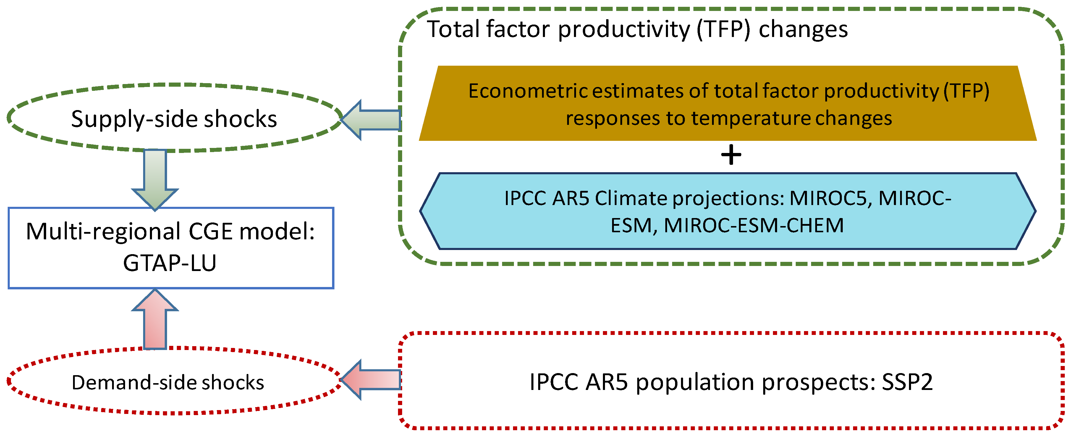
Near-term (i.e., by 2030) projected global warming impacts on agricultural production and the projected socioeconomic development were used as “shocks” on agricultural supply and demand flows. We adopted a neoclassical-style, medium-run closure for the simulation environment, wherein endowments of productive factors are fixed, market prices adjust endogenously to maintain full employment, and capital and labor are mobile between sectors, while land and natural resources are sector-specific. Figure 1 summarizes our research framework. In this study, we assumed the following about world development by 2030: (1) a socioeconomic scenario described in the Shared Socioeconomic Pathway 2 (SSP2) of the IPCC Fifth Assessment Report (AR5) which features modest global population and per-capita gross domestic product (GDP) growth and slow trade liberalization [23], relative to all SSPs; and (2) a climate scenario projected under the stabilizing Representative Concentration Pathway of greenhouse gas emissions (RCP 6.0) [24,25].
The SSP2 presents moderate expectations about population growth (The national population projections we adopted for SSP2 of the IPCC AR5 have factored in future trends in migration, as well as fertility, mortality, and educational transitions—which are critical in shaping the composition of national population (KC & Lutz, 2017) [26]. SS2, like SSP1 and SSP4, assumes medium-level migration trends, while SSP3 assumes low-level and SSP5 assumes high-level migration trends), urbanization, and spatial patterns of development. Specifically, it describes a world that develops, following historical patterns, at moderate rates of investment in human capital, technological change, and economic growth [27]. Further, population expansion augments demand for foods (by households) and for agricultural products thus derived. For the 2020–2039 period, temperature anomalies were taken from the Model for Interdisciplinary Research on Climate (MIROC5, see [28]), MIROC-ESM, and MIROC5-ESM-CHEM [29] general circulation models (GCM) projected climates, as per the Coupled Model Inter-Comparison Project’s fifth phase (CMIP5) [30]. To derive the supply-side shocks (i.e., the shocks on total factor productivity (TFP) in the GTAP-LU model), we coupled the MIROC temperature change projections with the agricultural yield changes in response to temperature deviations calculated by Roson and Satori (2016) [31]. The latter takes the estimated process-based reduced-form agricultural response function from Mendelsohn and Schlesinger (1999) [32] and extends Cline’s (2007) [33] work by calculating a single aggregated crop sector’s crop yield response to temperature change (An alternative measure to capture climate impact on agricultural productivity is through the Ricardian approach (Mendelsohn, Nordhaus, & Shaw, 1994) [34], which relates agricultural land values to climate variations. This approach has been applied to United States, Canada, India, and various African and Latin American countries (as summarized in Cline (2007) [33]). Among the few Ricardian analyses for Europe, De Salvo et al. (2013) [35] estimated the climate change impact on permanent crops in a small Italian Alpine region).
To implement the abovementioned scenario, we applied these exogenous shocks to the corresponding variables in the GTAP-LU model. In the model, since utility maximization of regional household consumption (specified over private and government expenditures, as well as savings) in the model is defined on a per capita basis, population growth affects aggregate regional utility and private household consumption expenditure on the demand side. On the supply side, the estimated crop yield changes are reflected by changes in the agricultural output-augmenting technological variables. The nested production function for a sector (j) of a region/country in the GTAP-LU model can be expressed in short as follows:
where Y indicates levels of gross output; X indicates intermediate input demand; E indicates employment of composite productive factors (including capital, labor, land and natural resources); A indicates output-augmenting technological change; and EF denotes demand for individual factors. Leontief and CES are the aggregators of the components in the form of a Leontief function and a Constant Elasticity of Substitution (CES) function, respectively. We imposed crop yield shocks, as derived from Roson and Satori (2016) [31], corresponding to the MIROC projections of temperature change, on the agricultural sector A variables.
Yj = Leontief (AjXij, AjEj), i = intermediate inputs, j = producing sectors,
Ej = CES (EFfj), f = productive factors,
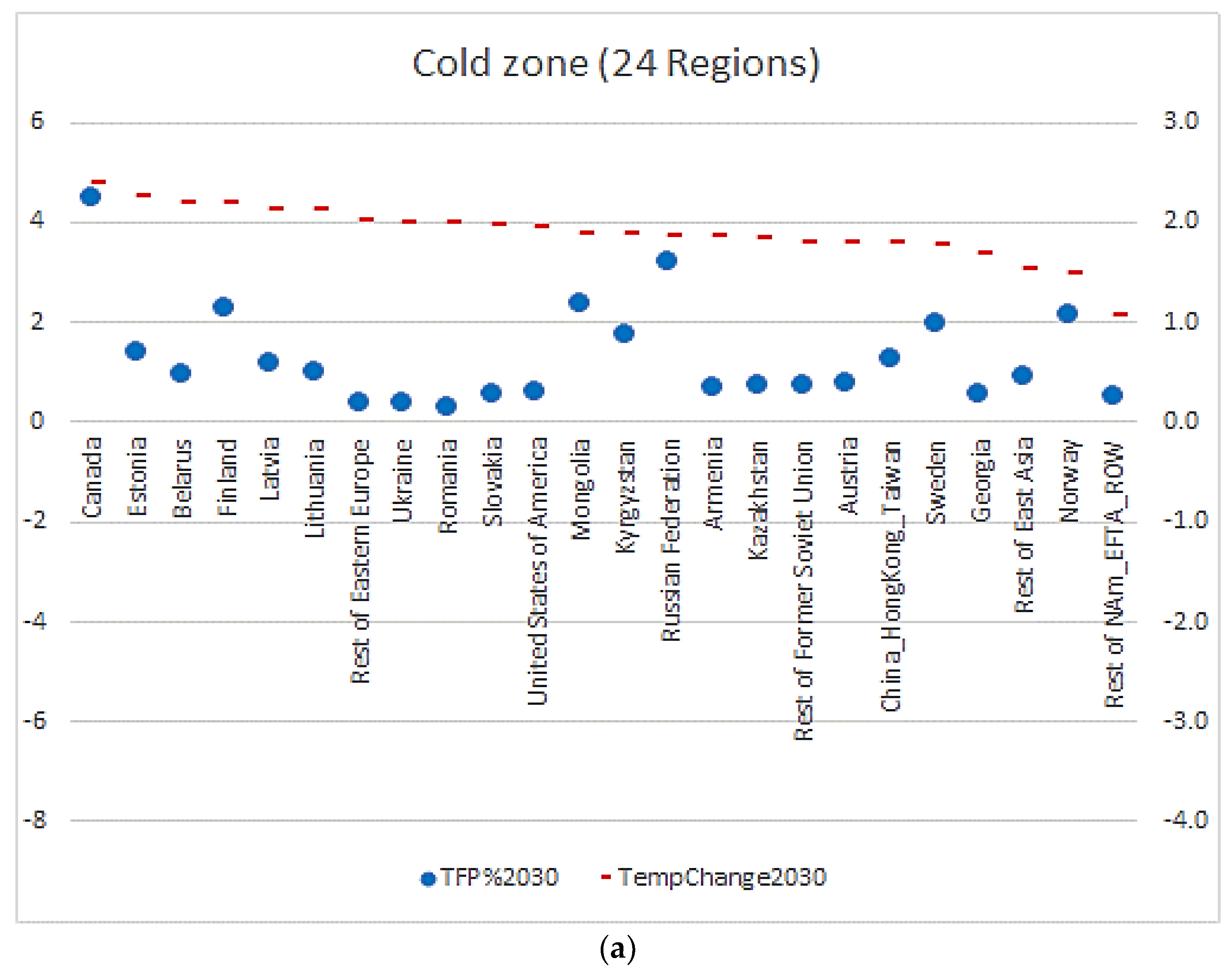
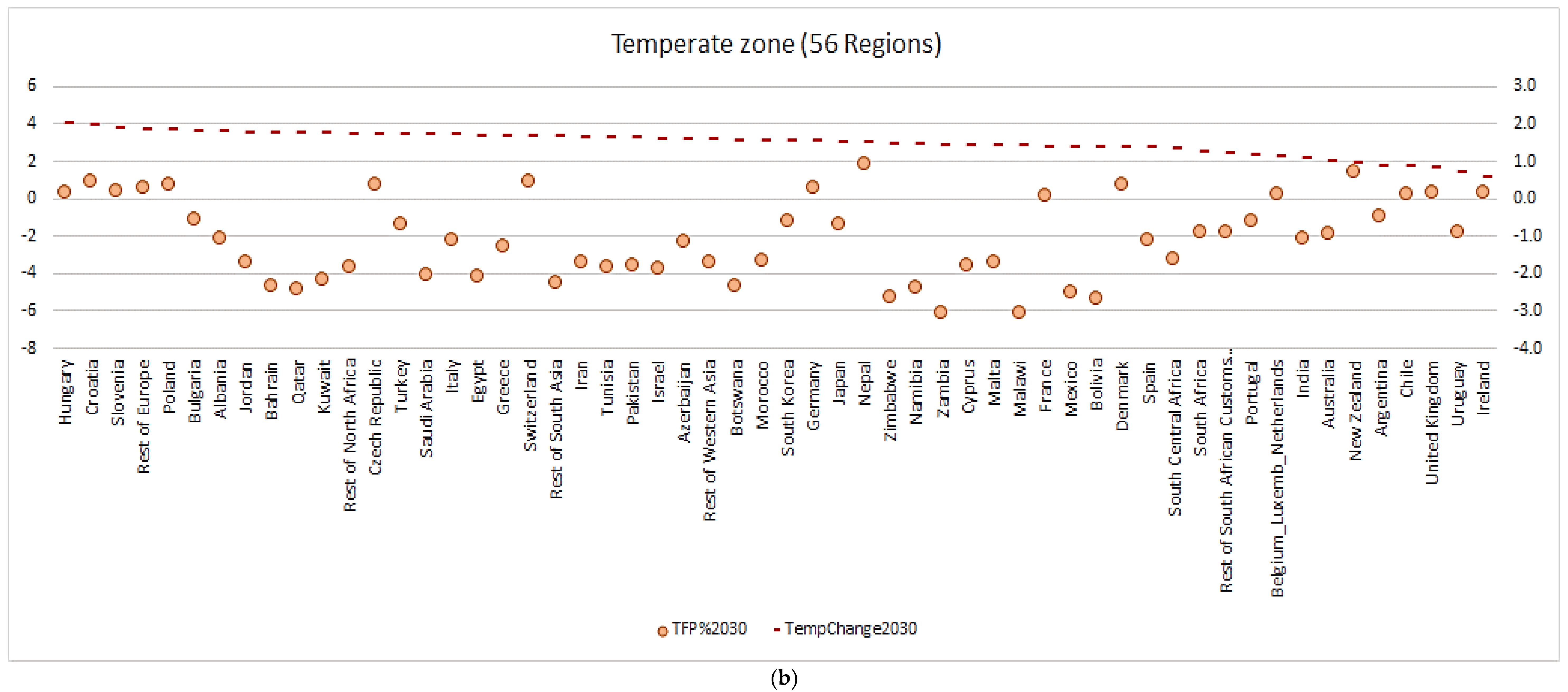
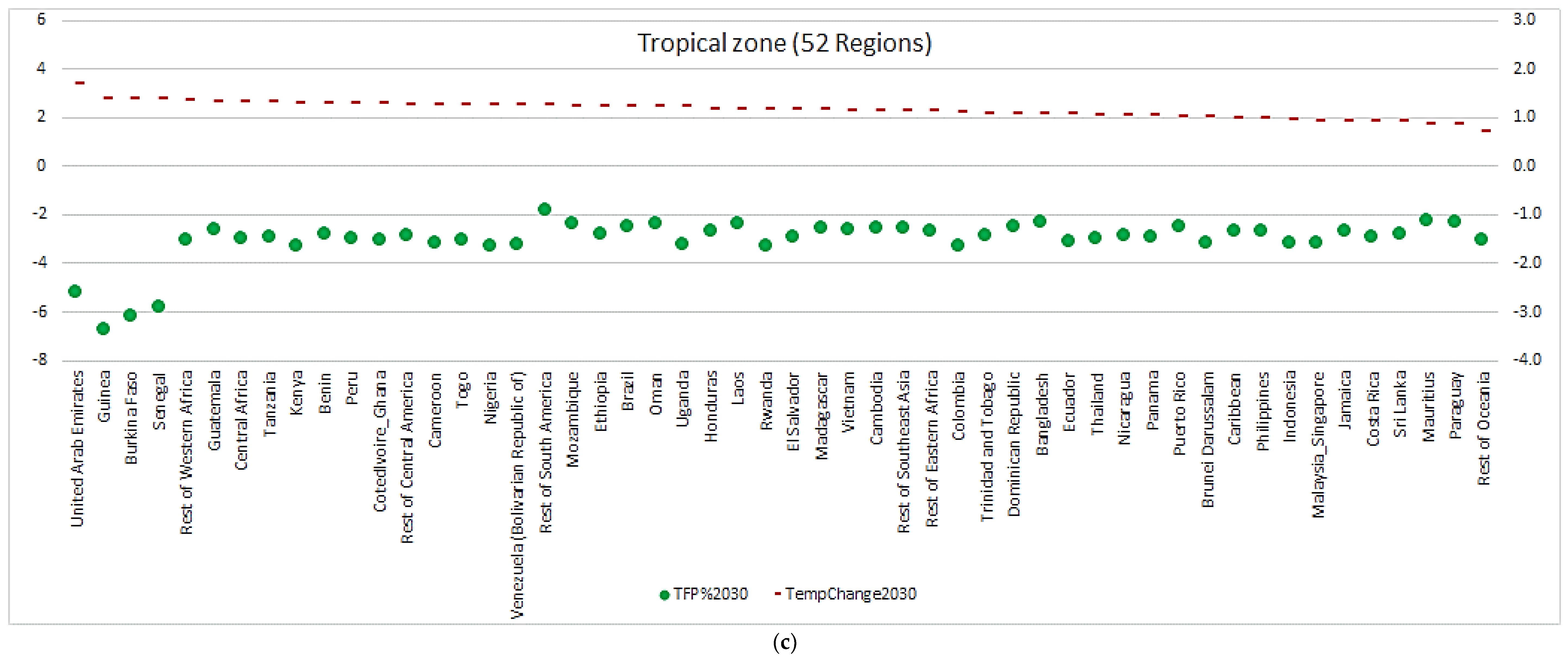
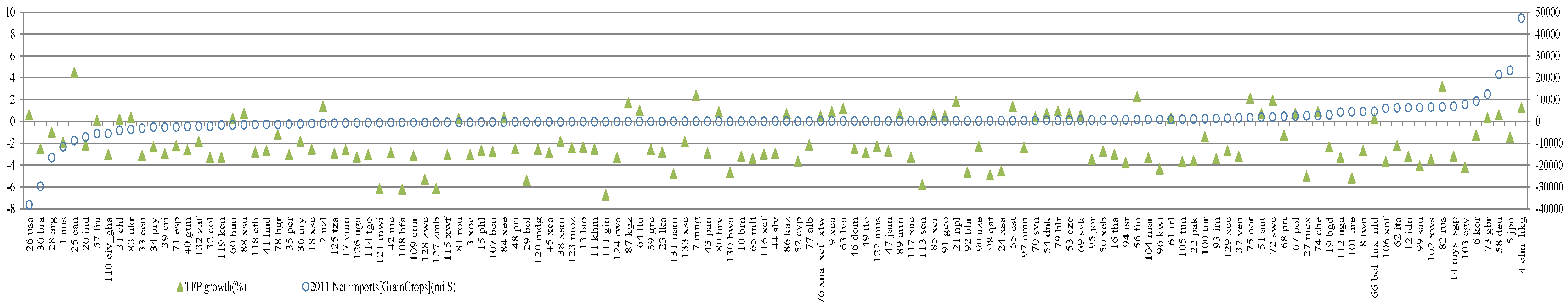
Figure 2a–c show the projected temperature changes and corresponding changes in crop yield that we incorporated into the GTAP-LU simulation for countries located in three climatic zones (i.e., cold, temperate, and tropical zones). Countries located in the cold zone are projected to have larger temperature increases than those in temperate and tropical zones. The corresponding crop TFP in cold zone countries (Figure 2a) is positive and of a larger magnitude than those positively affected countries in temperate and tropical zones. The majority of temperate zone countries (Figure 2b) and all of the tropical zone countries (Figure 2c) are subject to negative impacts on crop TFP. For these reasons, the positively affected cold-zone countries should be expected to assist those negatively affected countries through agricultural trade.
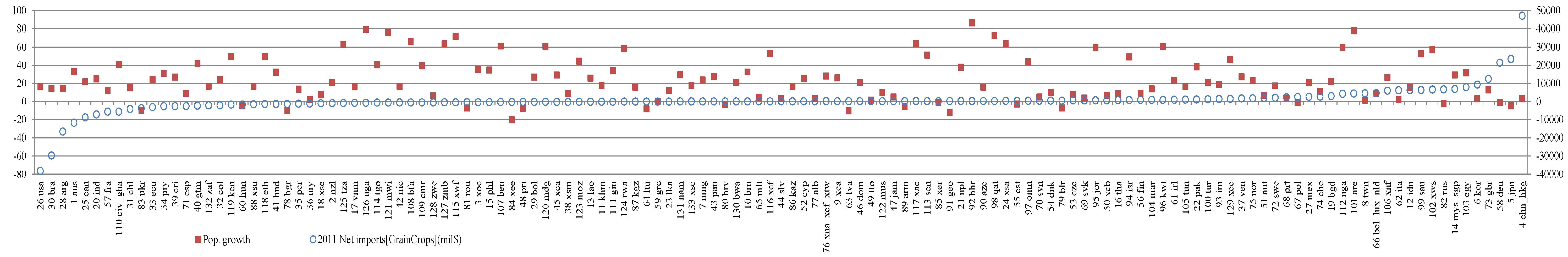
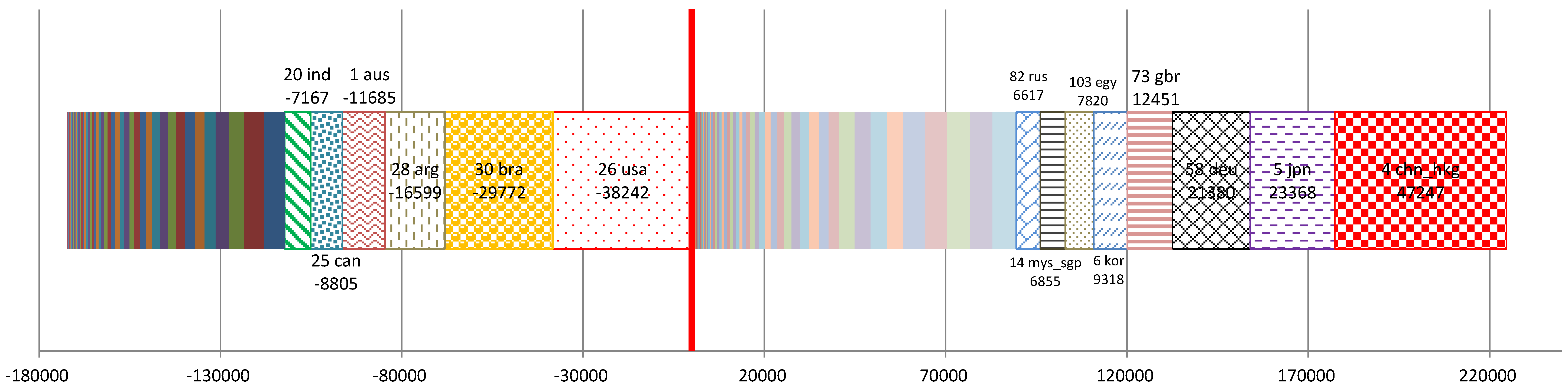
We sorted the countries by import volume of grain crops, as depicted in (a) Figure 3 by projected population growth, and (b) Figure 4 by TFP change (%) of the crop sector. Figure 5 shows the 2011 context of net importers and exporters of crops, ranked by volume (in million USD). As Figure 3 indicates, most of the 133 countries/regions will have expanded populations, with the exception of 18 countries, among which Ukraine (‘83 ukr’) is a top 10 net exporter of crops; and Japan (‘5 jpn’), Russia (‘82 rus’), and Germany (‘58 deu’) are top 8 net importers of crops.
Table 1 summarizes the projected population growth and crop TFP changes by 2030 for the top 10 net importers of crops, and Table 2 for the top 10 net exporters of crops. Population growth decrease helps alleviate the pressure for food demand placed on exporting countries by importing countries. If coupled with global warming-induced crop productivity improvements, this will further reduce food competition in the global market among importing countries. However, countries with such future prospects are limited to Germany and Russia, which both have negative population growth yet positive TFP changes from projected global warming (see Table 1). Germany will have a 1.14% population decrease by 2030, with a mild crop TFP improvement of 0.6%. The Russian population is projected to decrease 2.33% by 2030, with a 3.18% improvement in crop TFP. Though Japan’s population is projected to shrink 4.84% by 2030, global warming will decrease Japan’s crop TFP by 1.43%.
The majority of the top 10 crop net importers will have increased population growth, with growth magnitudes of at least 3% (e.g., China & Hong Kong, ‘4 chn_hkg’), and at most, 57.15% (Rest of Western Asia, ‘102 xws’). China & Hong Kong, and the United Kingdom (‘73 gbr’) comprise the top 1st and top 4th net importers of crops, respectively. The population of China & Hong Kong in 2011 accounted for nearly 20% of the world. A 3% expansion of the Chinese & Hong Kong population is equivalent to a 21% increase in the 2011 population of Brazil (‘30 bra’), which is the top 5th net importer of crops worldwide. Fortunately for net importers, China & Hong Kong—as well as the United Kingdom—is projected to have a 1.26% improvement in its crop TFP, which will slightly help alleviate pressure for crop demand in the global market. As shown in the third column of Table 1, the remaining top 10 net importers’ crop yields are projected to be negatively impacted, though population growth is projected to be significant, which will exert pressure on the global food demand.
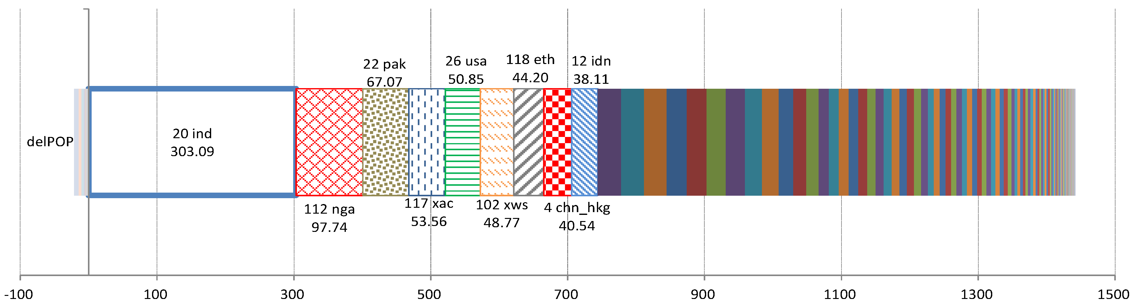
Among the top 10 net exporters (see Table 2), the only country with a projected decreased population is Ukraine, whose population is projected to reduce by 9.59% and crop TFP to increase by 0.37%. Ukraine, therefore, is expected to supply more crops to its foreign purchasers. Nine out of the top 10 net crop exporters will have much larger populations, with population growth magnitudes from 11.99% (France, ‘57 fra’) to 40.74% (Cote d’Ivoire & Ghana, ‘110 civ_gha’). Figure 6 shows the top contributors of global population expansion. Among the top 10 net crop exporters, India (‘20 ind’) will have an additional 303 million people, and the United States (‘26 usa’), an additional 51 million people. Because the majority of the countries with relatively large population expansion projections are net importers, the global food demand is expected to be impacted.
Unfortunately, the crop TFP of India (‘20 ind’), the country with the largest population expansion projection (see Figure 6), will be negatively affected by global warming at a magnitude of −2.17%. The other highly ranked net exporters of crops (see Figure 5), such as Brazil (‘30 bra’), Argentina (‘28 arg’), and Australia (‘1 aus’), also face TFP declines of 1.0–2.5% by 2030. This will further aggravate the global food shortage.
We incorporated the above-mentioned exogenous shocks into the GTAP land use model, which is aggregated into 12 sectors within 133 countries/regions. The sectoral and regional aggregation schemes are shown in Tables S1 and S2 (in Supplementary Information), respectively. In the GTAP land use model, the 133 economies respond to shocks (i.e., domestic demand, exports, prices, and output levels of crops and other commodities/services produced), while reaching a new equilibrium in which demand equals supply in all commodities/services markets of domestically produced and imported goods. The quantitative economic impact of temperature-induced crop yield changes by 2030 can be measured by the economic variable deviations from the initial equilibrium of the GTAP land use model (e.g., price, supply, and demand), which is calibrated to the 2011 benchmark data on multi-regional input-output accounts and bilateral trade.
4. Results
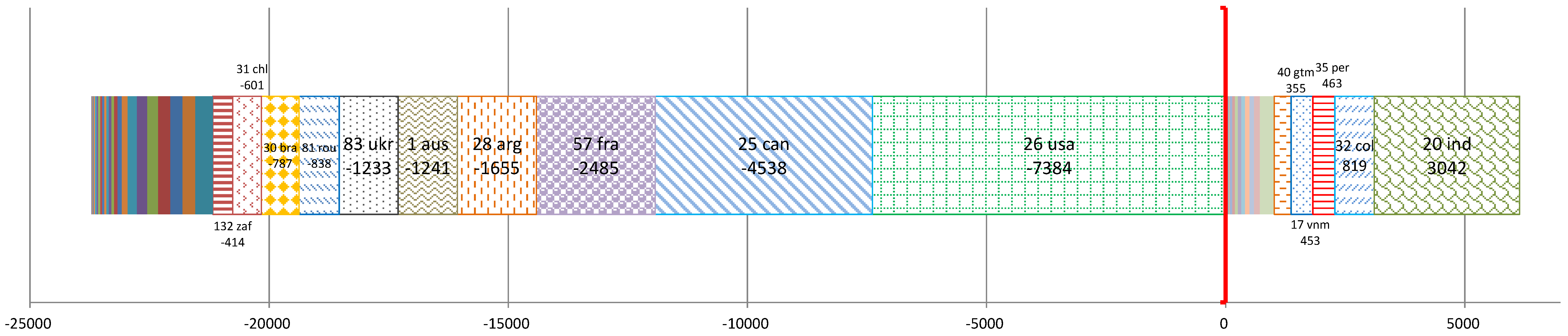
This study focuses on country-specific impacts on net import volume of crops. The model results for the endogenous variables are expressed in percentage change, indicating percentage deviation of post-shock values from pre-shock equilibrium. We then calculated the magnitude of change (e.g., in import volume) by multiplying the quantity and/or price variable percentage change (e.g., import demands and prices) with their corresponding model calibration benchmark data (e.g., pre-shock import expenditure). Figure 7 shows the simulated changes in net import volume of net exporters, while Figure 8 shows simulated changes in net import volume of net importers.
In Figure 7, net exporting countries with positive changes in net import volume (i.e., results to the right of the origin) reduce their net exports of crops, while those with negative changes (i.e., results to the left of the origin) expand their net exports. Net exporting countries with negative changes in Figure 7 are relatively mildly impacted by global warming, such that warming brings crop TFP improvements for the US (‘26 usa’), Canada (‘25 can’) and France (‘57 fra’), Ukraine (‘83 ukr’) and Chile (‘31 chl’), and mild decline for Argentina (‘28 arg’) and Australia (‘1 aus’). Countries with negative changes can expand their net exports, thus negatively changing their net import volume. Net exporting countries with positive changes in Figure 7 have relatively larger population expansion, further complicated by the relatively severe impact of global warming (e.g., India has the largest population expansion (see Figure 6) and a 2.17% decline in crop TFP). Thus, these countries would see a reduction in their net exports, and therefore, positive changes in net import volume.
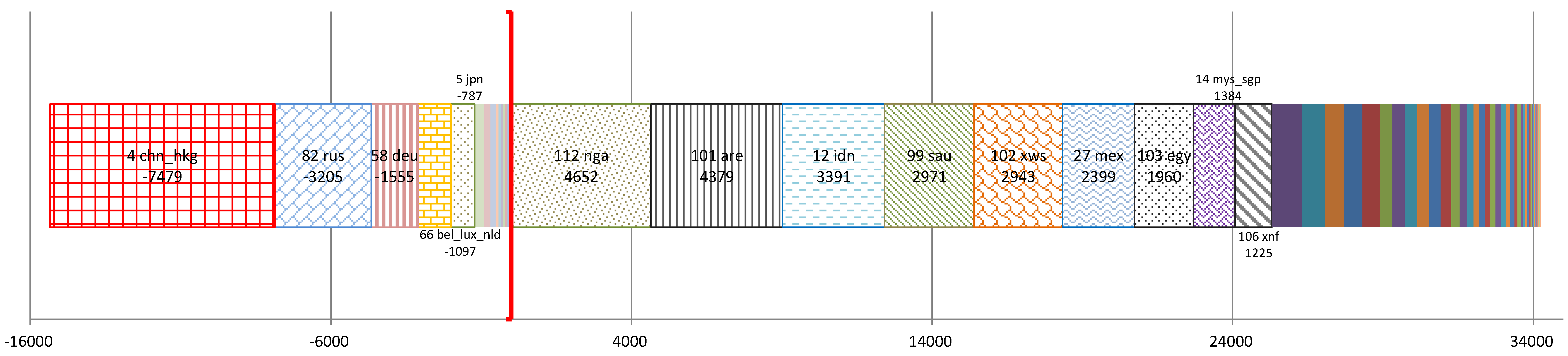
In Figure 8, net importing countries with negative changes in net import volume (i.e., results to the left of the origin) reduce their net imports of crops, while those with positive changes (i.e., results to the right of the origin) expand their net imports. Net importing countries with negative changes in Figure 8 are relatively mildly impacted by global warming, such that warming brings crop TFP improvement for China and Hong Kong (4 ‘chn_hkg’), Russia (‘82 rus’), Germany (‘58 deu’), and Belgium, Luxembourg, and the Netherlands (‘66 bel_lux_nld’). The net import decreases of Russia (‘82 rus’) and Germany (‘58 deu’) are further enabled by declining populations. China and Hong Kong face a relatively smaller expansion in population, with an expected 3% growth and a 1.26% increase of crop TFP, which results in China and Hong Kong seeing the most reduction in crop net imports for a single country, i.e., equivalent to $7.479 billion USD. The biggest reduction in population for a single country (i.e., a 4.84% decrease) turns Japan (‘5 jpn’) into a significantly smaller net importer, with a 1.43% decline in crop TFP. Apparently, the population effect outperforms the TFP effect.
Net importing countries with positive changes in Figure 8 (e.g., Nigeria (‘112 nga’), Indonesia (‘12 idn’), United Arab Emirates (‘101 are’), Saudi Arabia (‘99 sau’), Rest of Western Asia (‘102 xws’), Mexico (‘27 mex’), Egypt (‘103 egy’), Malaysia and Singapore (‘14 mys_sgp’), and Rest of North Africa (‘106 xnf’) expand their net imports due to relatively severe declines in crop TFP, while large population increases (as shown in Figure 6) further contribute to the larger net import expansion of, for example, Nigeria (‘112 nga’) and Indonesia (‘12 idn’).
Four countries invert roles, changing from net exporters to net importers as a result of the TFP and population growth impacts by 2030, including the Philippines (‘15 phl’), Sri Lanka (‘23 lka’), and Panama (‘43 pan’). These three countries contribute to a $1.259 billion USD in total expansion in global net import demand. The Philippines changes from a net exporter worth $589 million USD to a net importer worth $389 million USD. This is due to sizable population expansion coupled with an adverse impact from global warming on crop TFP (i.e., 2.68% decrease). Sri Lanka changes from a net exporter worth $157 million USD to a net importer of $65 million USD, due to adverse impacts from global warming on crop TFP (i.e., 2.8% decrease). Panama changes from a net exporter worth $17 million USD to a net importer worth $43 million USD, also due to adverse impacts from global warming on crop TFP (i.e., 2.9% decrease). Latvia (‘63 lva’) changes from a net importer worth $69 million USD into a net exporter worth $9 million USD as a result of their projected population reduction (i.e., 0.21% decrease) and a 1.18% increase in crop TFP, resulting in a $78 million USD reduction in net imports.
A total expansion of $24.324 billion USD in net exports by the countries with negative changes in Figure 7 surpasses the $7.083 billion USD of total net export reduction by the countries with positive changes, resulting in a net increase of $17.241 billion USD in the global net export volume of crops. In Figure 8, the total expansion in net imports of the countries with positive changes (i.e., $31.335 billion USD) surpasses the $14.094 billion USD of total net import reduction, which generates a net increase of $17.241 billion USD in the global net import volume of crops. The net increase in global net import volume corresponds to the net increase in global net exports, with both values being $17.241 billion USD. In sum, the volume of crops increases by $47.345 billion USD, with the effects of global warming-induced crop TFP change coupled with the demand push from global population expansion.
To put the global crop import demand expansion (i.e., $47.345 billion USD increase) and its equivalent global crop export supply into perspective, this amount is equivalent to: the sum of Brazil and China’s 2011 crop exports; the sum of Canada, Argentina, and Australia’s 2011 crop exports; or the sum of Japan, U.K., and Italy’s 2011 crop imports. This indicates that the projected populations, together with the global warming-induced crop TFP changes by 2030 for all the countries/regions, result in significant pressure being placed on global land resources, which drives price inflation in the global food markets. The $47.345 billion USD expansion of the global crop export supply is a 6.4% increase in volume and a 4.9% rise in the average price of global crop exports. This is supported by an increase in crop output globally. At the aggregate level, global warming brings a 4.46% increase in global crop output, so that the global average price index for crop output rises by 6.75%.
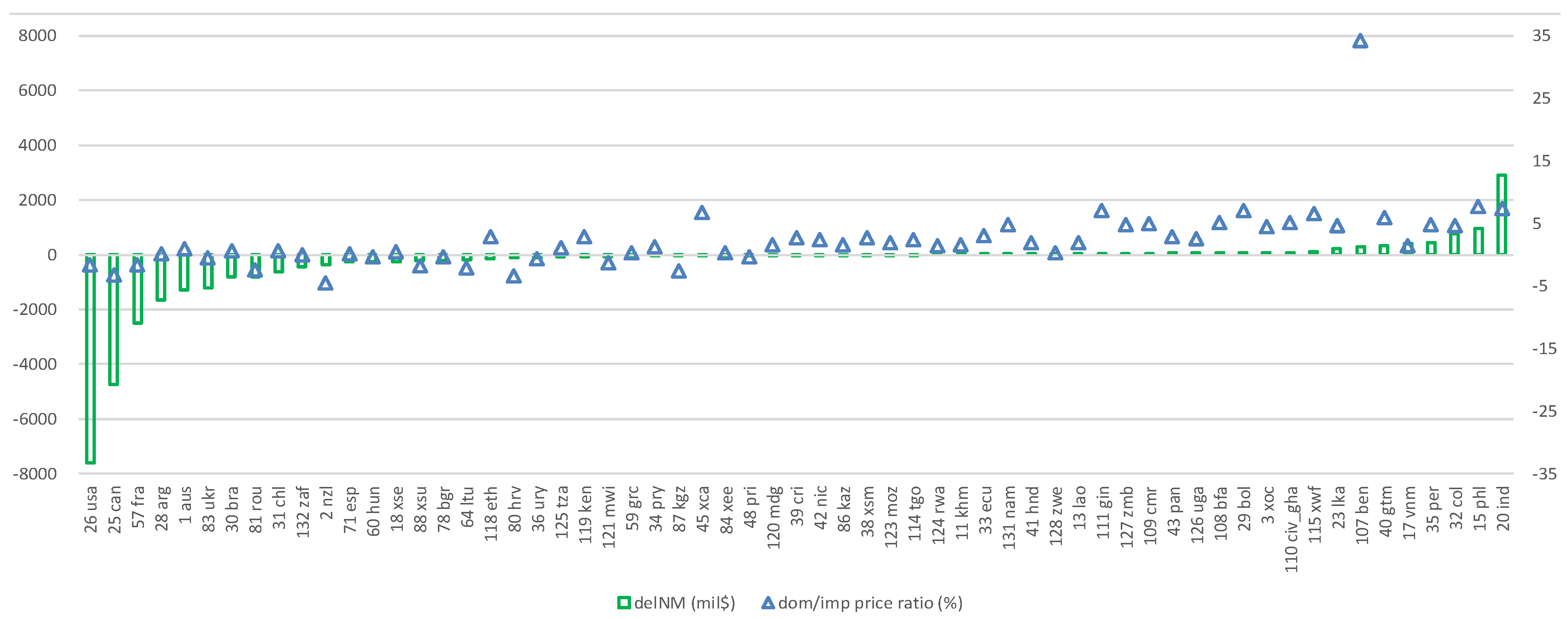
However, the spatially heterogeneous impact of warming on the crop TFP in combination with country-specific population projections would give rise to varying market consequences for individual countries. Figure 9 shows changes in the domestic/import relative price ratio for net exporters. In Figure 9, ‘delNM’ indicates change in net import volume of the net exporter. Positive ‘delNM’ refers to reduction in volume of crop net exports, while negative ‘delNM’ refers to an increase in net exports corresponding to the exogenous shocks specified in the simulation. The United States and Canada increase their net export volume of crops, while India and the Philippines’ net crop exports reduce. For each country, its net crop export volume adjusts corresponding to the change in the domestic/import price ratio at equilibrium. A net exporter would see reduction in its net export volume of crops if domestic crop price rises relatively more than its imported counterpart, and vice versa. In Figure 9, net exporters on the extreme right have positive changes in the domestic/import price ratio of crops, and therefore, their net crop exports decline (positive change in net imports). Net exporters on the extreme left, however, have negative or near zero change in the domestic/import price ratio of crops, so their net crop exports increase.
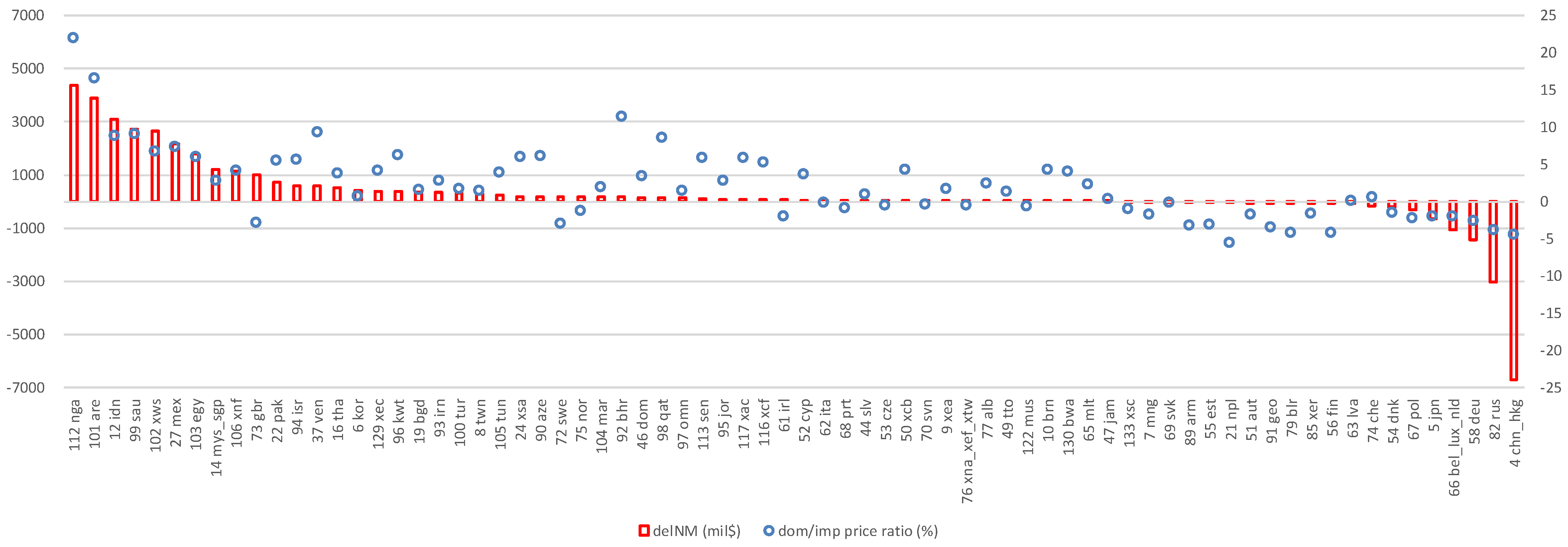
Figure 10 shows changes in the domestic/import relative price ratio for the net importers. A positive ‘delNM’ indicates larger volume of net crop imports, while a negative ‘delNM’ indicates a smaller volume of net imports corresponding to the exogenous shocks specified in the simulation. Nigeria (‘112 nga’), United Arab Emirates (‘101 are’), and Indonesia (‘12 idn’) increase their net import volume of crops, while China and Hong Kong (4 chn_hkg), and Russia (82 rus) reduce net crop imports. A net importer increases its net import volume of crops if domestic crop prices rise relatively more than those of their imported counterparts, and vice versa. In Figure 10, net importers on the extreme right have negative changes in their domestic/import crop price ratio; therefore, their net crop imports decline. Net importers on the extreme left have positive or close to zero change in the domestic/import crop price ratio, so their net crop imports increase.
5. Discussion
A complex interplay of demographics, climatic conditions, economics, technology, and trade will continue to impact food security with certain countries and regions expected to fare better. Unfortunately, according to the results of this study and a number of other studies (such as [1,36,37]), many factors may predispose developing countries and regions to experience greater adversity in food security than developed countries. Despite this, forecasted poverty reductions may increase financial viability and agricultural productivity by allowing for increased intensification through technological acquisition or advancement. Increases in wealth may also strengthen trade while appropriate trade policies may alleviate many of the predicted shortcomings that developing countries will experience [8]. Moreover, Monier et al. (2018) [38] indicate that few theories attempt to directly translate the impacts of global mean temperature change to GDP. Yet, Chalise and Naranpanawa (2016) [39] reported that overall, the Nepalese economy was significantly and negatively impacted by climate change-induced agricultural productivity losses, and indicated an urgent need to mainstream adaptation and mitigation strategies based on the results of a country-specific CGE model. Cai et al. (2016) [40] suggested that climate change can significantly reduce food production (relative to historical trends), and can create upward pressure on food prices, resulting in adverse food security impacts in the South Asian region. The findings of this study reveal that the food security of individual countries is highly context specific, and while certain conditions may increase susceptibility to or likelihood of food security issues, none predetermine this outcome. Instead, food security issues can be mitigated as long as the specific circumstances of individual countries are considered.
One important factor to consider is the locations of surplus food production and food demand, given projected climate change and demographic trends such as those of recent studies [10,38,40]. According to the results of this study, current net exporting countries whose TFP is favorably impacted by climate change up to 2030 are predominantly located in cooler temperate climatic zones, e.g., the United States and Canada. Countries located in these regions will be able to increase their crop exports. However, other net exporters may decrease exports due to climatically unfavorable conditions or demographic changes. Take, for example, India and the Philippines, which are located in temperate and tropical zones, respectively. Both of these countries are expected to reduce their exports due to unfavorable TFP conditions and greater domestic demand due to population growth. Fortunately, other net importing countries, whose TFP are favorably impacted by climate change, may be able to reduce their crop import demands, e.g., China and Russia. On the other hand, others may need to increase their net imports over and above current deficiencies as they continue to experience the negative impacts of both climate and demographic change. For example, the TFP of Nigeria and Indonesia will be negatively impacted by climate, and the situation will be compounded as their populations continue to increase.
From these results, our study demonstrates the relationship that domestic demand (which is linked to population growth) and domestic supply (which is linked to TFP changes) has with exports. In general, those countries that have projected decreasing or stable populations and favorable climatic conditions can increase net exports—or, at the very least, decrease net imports. However, net exporting countries with increasing populations (see Figure 7 and Table 2) will need to decrease exports, particularly if agricultural conditions are also negatively impacted by global warming, e.g., India has the largest population increase (see Figure 6) and a 2.17% decline in crop TFP. Moreover, at a local scale, population increases may drive up crop demand, and thus a requisite land demand, increasing land rent and vice versa [3]. Taken as a whole, our results indicate that the 2030 population projections, together with the global warming-induced crop TFP modeled changes, result in significant pressure on global land resources, which may drive up inflation in the global food markets.
Nelson et al. (2014) [1] reported that in response to climate change, agricultural production, cropland area, trade, and prices are significantly varied. Countries that are relatively less affected by climate change, however, may benefit from trade gains [9]. As may be expected, the above fluctuations in supply and demand at the national level have cascading effects on market prices. For example, due to predicted decreases in surpluses on both the local and global scales, consumer prices have been projected to increase under climate change [8]. Unlike Ray (2015) [41], who gave a spatially-detailed account of the global distribution of crop yields and variation, as well as the degree to which this was driven by climate variability, results from the GTAP-LU model used in this study indicate a projected increased volume of global crop exports, as well as average prices. This is supported by an overall increase in crop output globally, which, nonetheless, fail to keep up with growing demand (cf. Figure 9 and Figure 10). However, the spatially heterogeneous impact of warming on crop TFP, in combination with country-specific population growth and market conditions, may give rise to varying market consequences for individual countries. Simply put, the net crop export volume adjustments of each country correspond to fluctuations in the domestic/import price ratio at equilibrium. For example, a net exporter would reduce net crop export volume if they could get a better price domestically and vice versa. In general, net exporting countries are projected to be better off due to increased farm income as their crop exports increase to meet the demand from net importing countries.
Our results indicate that the global income gap may increase between the Global South and the Global North, since projections show that the majority of the South is subject to crop yield reductions, while the developed North will experience favorable rising crop yields. Regardless of how equitable this may be—e.g., many of the developed countries have released greater amounts of greenhouse gasses, and yet appear to profit most from global warming—under the current market economy, trade seems to be an essential factor in securing global food security. As Mauser et al. (2015) [3] suggested, there is greater potential for achieving food security when investment in present-day cropland management improvements consider all interlinked effects.
For net importing countries, in particular, policy measures aimed at effectively alleviating food security issues should also take into account the geographically diverse impact of climate change on crop exporting countries, particularly their current sources of crop imports. Therefore, by improving climate change effects on food security projections at the national scale, our study offers a comprehensive and high-resolution picture of prospective global food markets. This can help in informing and assisting individual countries in instituting precautionary national-level policy measures and action plans aimed at alleviating food insecurity and combating pressure from food price inflation [4,6,7].
To reiterate our current reality, increasing overall global food security largely depends on the continued reliance between countries in securing their economic and food security welfare. This means meeting the domestic food demand for net importing countries and raising agricultural incomes for net exporting countries. Despite this, further research is needed to assess the trade-offs between agricultural intensification and its impacts on ecosystems (e.g., biodiversity, carbon stocks and flows), as well as the social aspects involved when forests, pasture, or previously unused areas become cropland [3]. Although CGE modelling is generally used for this type of research [39,40,42,43] and has analytical advantages for use in making economic assessments of the effects of climate change and evaluating climate policy efficacy, other models should be used to compare the impacts of climate change, since CGE models rely on different databases [1]. To improve future models, model integration under a common data exchange protocol also has great potential [1]. Finally, our study is based on the RCP 6.0 scenario for the 2020 to 2039 period. However, Nelson et al. (2014) [1] indicated that the upper end of climate change’s direct yield effects can be arrived at using the most extreme RCP representing negative productivity effects.
6. Conclusions
The effects of climate change on agricultural production and food security are manifold. This study provides a comprehensive economic assessment for global agriculture in the context of a global temperature rise by 2030, as projected under the socioeconomic pathway SSP2 and representative concentration pathway RCP 6.0. By simulating a comprehensive set of 133 world countries/regions, we forecasted disturbances in the current pattern of global agricultural trade. In particular, we showed the change in country-specific net import demand and net export supply of crops as a result of the spatially diverse impacts on the agricultural total factor productivity of the projected climate and socioeconomic scenarios in 2030. Our analysis offers a comprehensive, high-resolution picture of the projected global food market to inform and assist countries in their national decision-making processes while facing food insecurity and food price inflation eventualities.
The projected population scenarios, together with the global warming-induced crop TFP changes by 2030 for all countries/regions, demonstrate the significant pressure that will be exerted on land resources thus driving up price inflation in the global food markets, and in particular, in countries with negative crop yield impacts. Under such a scenario, our simulation results in a $47.345 billion USD increase in global crop export supply, which is the result of a 6.4% and a 4.9% rise in the global crop export volume and average price, respectively. The increase in global aggregate crop output (i.e., 4.46% increase) facilitated such export expansion. However, at equilibrium, the global average price index for crop output rises by 6.75%. Pressure from the demand side due to population expansion contributes to this rise in global average crop price, suggesting an increased financial burden by 2030 to feed, in particular, net importing countries. On the other hand, net exporting countries are projected to become better off, with increased farm income as their crop exports expand to meet the demand from net importing countries.
This study also investigated individual countries and found that current net exporting countries whose TFP is favorably impacted by the temperature rise by 2030, and which are located in cold climatic zones, will be able to expand their crop exports (e.g., United Stated and Canada). However, India and the Philippines, which are located in temperate and tropical zones respectively, will reduce their exports due to unfavorable TFP impacts and also increased population. Current net importing countries whose TFP are favorably impacted by the temperature rise by 2030 will be able to reduce their crop import demands (e.g., China and Russia). On the other hand, Nigeria and Indonesia, which will have negative TFP impacts and sizable population increases by 2030, will largely increase their net crop imports. Our model results also suggest the likely widening of the global income gap between developing countries and industrialized countries, a consequence of the geographically heterogeneous distributed shocks simulated in this study.
The impact of climate change occurring in one region, be it positive or negative, overflows into other regions by way of trade. The projected intensified global agricultural trade suggests increased reliance between countries in securing economic welfare, which is enabled when the domestic food demand for net importing countries is met, thereby raising farm income for net exporting countries. Depending on the position and the nodal relationship of each country in the global agricultural trade network, countries may experience the heterogeneous economic consequences of global warming. National and international policy measures aimed at effectively alleviating net importing countries’ food security issues should also consider how global crop yields are geographically and diversely impacted by climate change. With this study, we present an outlook of regional realities by 2030 for present-day considerations.
Supplementary Materials
The following are available online at https://www.mdpi.com/2071-1050/10/8/2763/s1, Figure S1: Production structure of the agricultural sectors, Figure S2: Nesting structure for AEZ-specific land supply, Table S1: Sectoral aggregation scheme for the GTAP database: 12 sectors, Table S2: Country aggregation scheme for the GTAP database: 133 countries/regions.
Author Contributions
The scope of this study was developed by Huey-Lin Lee and Yu-Pin Lin. The first manuscript draft was written by Huey-Lin Lee and Yu-Pin Lin, and was substantially revised by Huey-Lin Lee and Yu-Pin Lin and J.R. Petway. The modeling work was done by Huey-Lin Lee and was discussed with Yu-Pin Lin.
Acknowledgments
The authors would like to thank the National Science Council of the Republic of China, Taiwan, for financially supporting this research under Contract Nos. 105-2621-M-002 -003 -MY3, 105-2621-M-004-002-MY3 and 103-2410-H-002 -161 -MY3.
Conflicts of Interest
No conflicts of interest.
References
- Nelson, G.C.; Valin, H.; Sands, R.D.; Havlík, P.; Ahammad, H.; Deryng, D.; Elliott, J.; Fujimori, S.; Hasegawa, T.; Heyhoe, E.; et al. Climate change effects on agriculture: Economic responses to biophysical shocks. Proc. Natl. Acad. Sci. USA 2014, 111, 3274–3279. [Google Scholar] [CrossRef] [PubMed] [Green Version]
- Ciscar, J.-C.; Iglesias, A.; Feyen, L.; Szabó, L.; Van Regemorter, D.; Amelung, B.; Nicholls, R.; Watkiss, P.; Christensen, O.N.; Dankers, R.; et al. Physical and economic consequences of climate change in Europe. Proc. Natl. Acad. Sci. USA 2017, 7, 2678–2683. [Google Scholar] [CrossRef] [PubMed] [Green Version]
- Mauser, W.; Klepper, G.; Zabel, F.; Delzeit, R.; Hank, T.; Putzenlechner, B.; Calzadilla, A. Global biomass production potentials exceed expected future demand without the need for cropland expansion. Nat. Commun. 2015, 6, 8946. [Google Scholar] [CrossRef] [PubMed]
- Wheeler, T.; Von Braun, J. Climate change impacts on global food security. Science 2013, 341, 508–513. [Google Scholar] [CrossRef] [PubMed]
- Lipper, L.; Thornton, P.; Campbell, B.M.; Baedeker, T.; Braimoh, A.; Bwalya, M.; Caron, P.; Cattaneo, A.; Garrity, D.P.; Henry, K.; et al. Climate-smart agriculture for food security. Nat. Clim. Chang. 2014, 4, 1068. [Google Scholar] [CrossRef]
- Bryan, B.A.; Nolan, M.; McKellar, L.; Connor, J.D.; Newth, D.; Harwood, T.; King, D.; Navarro, J.; Cai, Y.; Gao, L.; et al. Land-use and sustainability under intersecting global change and domestic policy scenarios: Trajectories for Australia to 2050. Glob. Environ. Chang. 2016, 38, 130–152. [Google Scholar] [CrossRef]
- Xu, Z.; Tang, Y.; Connor, T.; Li, D.; Li, Y.; Liu, J. Climate variability and trends at a national scale. Sci. Rep. 2017, 7, 3258. [Google Scholar] [CrossRef] [PubMed]
- Stevanović, M.; Popp, A.; Lotze-Campen, H.; Dietrich, J.P.; Müller, C.; Bonsch, M.; Schmitz, C.; Bodirsky, B.L.; Humpenöder, F.; Weindl, I. The impact of high-end climate change on agricultural welfare. Sci. Adv. 2016, 2, e1501452. [Google Scholar] [CrossRef] [PubMed] [Green Version]
- Dellink, R.; Lanzi, E.; Chateau, J. The Sectoral and Regional Economic Consequences of Climate Change to 2060. Environ. Resour. Econ. 2017, 1–55. [Google Scholar] [CrossRef]
- Chalise, S.; Naranpanawa, A.; Bandara, J.S.; Sarker, T. A general equilibrium assessment of climate change–induced loss of agricultural productivity in Nepal. Econ. Model. 2017, 62, 43–50. [Google Scholar] [CrossRef]
- Eboli, F.; Parrado, R.; Roson, R. Climate-change feedback on economic growth: explorations with a dynamic general equilibrium model. Environ. Dev. Econ. 2010, 15, 515–533. [Google Scholar] [CrossRef] [Green Version]
- Bosello, F.; Eboli, F.; Pierfederici, R. Assessing the Economic Impacts of Climate Change. An Updated CGE Point of View; FEEM Working Paper, No. 2.2012; Centro Euro-Mediterraneo sui Cambiamenti Climatici: Venice, Italy, 2012. [Google Scholar]
- Roson, R.; Van der Mensbrugghe, D. Climate change and economic growth: impacts and interactions. Int. J. Sustain. Econ. 2012, 4, 270–285. [Google Scholar] [CrossRef]
- Bosello, F.; Parrado, R. Climate Change Impacts and Market Driven Adaptation: The Costs of Inaction Including Market Rigidities; FEEM Working Paper, No. 64. 2014; Ca’ Foscari University of Venice: Venice, Italy, 2014. [Google Scholar]
- Aguiar, A.; Narayanan, B.; McDougall, R. An Overview of the GTAP 9 Data Base. J. Glob. Econ. Anal. 2016, 1, 181–208. [Google Scholar] [CrossRef] [Green Version]
- Lee, H.L. The Impact of Climate Change on Global Food Supply and Demand, Food Prices, and Land Use. Paddy Water Environ. 2009, 7, 321–331. [Google Scholar] [CrossRef]
- Hertel, T.W. (Ed.) Global Trade Analysis: Modeling and Applications; Cambridge University Press: Cambridge, UK, 1997. [Google Scholar]
- Lee, H.L.; Hertel, T.W.; Rose, S.; Avetisyan, M. An integrated global land use data base for CGE analysis of climate policy options. In Economic Analysis of Land Use in Global Climate Change Policy; Hertel, T.W., Rose, S.K., Tol, R.S.J., Eds.; Routledge: Abingdon, UK, 2009; pp. 72–88. [Google Scholar]
- Baldos, U.L. Development of GTAP Version 9 Land Use and Land Cover Database for Years 2004, 2007 and 2011; Global Trade Analysis Project (GTAP), Department of Agricultural Economics, Purdue University: West Lafayette, IN, USA, 2017. [Google Scholar]
- Schmitz, C.; van Meijl, H.; Kyle, P.; Nelson, G.C.; Fujimori, S.; Gurgel, A.; Havlik, P.; Heyhoe, E.; Mason d’Croz, D.; Popp, A.; et al. Land-use change trajectories up to 2050: Insights from a global agro-economic model comparison. Agric. Econ. 2014, 45, 69–84. [Google Scholar] [CrossRef]
- Di Gregorio, A. Land Cover Classification System: Classification Concepts and User Manual; Food and Agriculture Organization of the United Nations: Rome, Italy, 2005. [Google Scholar]
- Dimaranan, B.V. Global Trade, Assistance, and Production: The GTAP 6 Data Base; Center for Global Trade Analysis, Purdue University: West Lafayette, IN, USA, 2004. [Google Scholar]
- O’Neill, B.C.; Kriegler, E.; Riahi, K.; Ebi, K.L.; Hallegatte, S.; Carter, T.R.; Mathur, R.; van Vuuren, D.P. A new scenario framework for climate change research: the concept of shared socio-economic pathways. Clim. Chang. 2014, 122, 387–400. [Google Scholar]
- Meinshausen, M.; Smith, S.J.; Calvin, K.; Daniel, J.S.; Kainuma, M.L.T.; Lamarque, J.-F.; Matsumoto, L.K.; Montzka, S.A.; Raper, S.C.B.; Riahi, K.; et al. The RCP greenhouse gas concentrations and their extensions from 1765 to 2300. Clim. Chang. 2011, 109, 213. [Google Scholar] [CrossRef]
- Intergovernmental Panel on Climate Change (IPCC). Climate Change: Impacts, Adaptation, and Vulnerability. Part A: Global and Sectoral Aspects. Contribution of Working Group II to The Fifth Assessment Report of The Intergovernmental Panel on Climate Change; Field, C.B., Vicente, R.B., Dokken, D.J., Pachauri, R.K., Allen, M.R., Barros, V.R., Broome, J., Cramer, W., Christ, R., Church, J.A., et al., Eds.; Cambridge University Press: Cambridge, UK, 2014. [Google Scholar]
- Samir, K.C.; Lutz, W. The human core of the shared socioeconomic pathways: Population scenarios by age, sex and level of education for all countries to 2100. Glob. Environ. Chang. 2017, 42, 181–192. [Google Scholar] [Green Version]
- Jones, B.; O’Neill, B.C. Spatially explicit global population scenarios consistent with the Shared Socioeconomic Pathways. Environ. Res. Lett. 2016, 11, 084003. [Google Scholar] [CrossRef] [Green Version]
- Watanabe, M.; Suzuki, T.; O’ishi, R.; Komuro, Y.; Watanabe, S.; Emori, S.; Takemura, T.; Chikira, M.; Ogura, T.; Sekiguchi, M.; et al. Improved Climate Simulation by MIROC5: Mean States, Variability, and Climate Sensitivity. J. Clim. 2012, 23, 6312–6335. [Google Scholar] [CrossRef]
- Watanabe, S.; Hajima, T.; Sudo, K.; Nagashima, T.; Takemura, T.; Okajima, H.; Nozawa, T.; Kawase, H.; Abe, M.; Yokohata, T.; et al. MIROC-ESM2010: Model description and basic results of CMIP5-20c3m experiments. Geosci. Model Dev. 2011, 4, 845. [Google Scholar] [CrossRef]
- Taylor, K.E.; Stouffer, R.J.; Meehl, G.A. An Overview of CMIP5 and the Experiment Design. Bull. Am. Meteorol. Soc. 2012, 93, 485–498. [Google Scholar] [CrossRef] [Green Version]
- Roson, R.; Sartori, M. Estimation of Climate Change Damage Functions for 140 Regions in the GTAP 9 Data Base. World Bank 2016, 1, 38. [Google Scholar]
- Mendelsohn, R.; Schlesinger, M.E. Climate-response functions. Ambio 1999, 28, 362–366. [Google Scholar]
- Cline, W.R. Global Warming and Agriculture: Impact Estimates by Country; Columbia University Press: New York, NY, USA, 2007. [Google Scholar]
- Mendelsohn, R.; Nordhaus, W.D.; Shaw, D. The Impact of Global Warming on Agriculture: A Ricardian Analysis. Am. Econ. Rev. 1994, 84, 753–771. [Google Scholar]
- De Salvo, M.; Raffaelli, R.; Moser, R. The impact of climate change on permanent crops in an Alpine region: A Ricardian analysis. Agric. Syst. 2013, 118, 23–32. [Google Scholar] [CrossRef]
- Wesseh, P.K., Jr.; Lin, B. Climate change and agriculture under CO2 fertilization effects and farm level adaptation: Where do the models meet? Appl. Energy 2017, 195, 556–571. [Google Scholar] [CrossRef]
- Lin, Y.P.; Settele, J.; Petway, J.R. Ecoregional and Archetypical Considerations for National Responses to Food Security under Climate Change. Environments 2018, 5, 32. [Google Scholar] [CrossRef]
- Monier, E.; Paltsev, S.; Sokolov, A.; Chen, Y.H.H.; Gao, X.; Ejaz, Q.; Couzo, E.; Schlosser, C.A.; Dutkiewicz, S.; Fant, C.; et al. Toward a consistent modeling framework to assess multi-sectoral climate impacts. Nat. Commun. 2018, 9, 660. [Google Scholar] [CrossRef] [PubMed]
- Chalise, S.; Naranpanawa, A. Climate change adaptation in agriculture: A computable general equilibrium analysis of land-use change in Nepal. Land Use Policy 2016, 59, 241–250. [Google Scholar] [CrossRef]
- Cai, Y.; Bandara, J.S.; Newth, D. A framework for integrated assessment of food production economics in South Asia under climate change. Environ. Model. Softw. 2016, 75, 459–497. [Google Scholar] [CrossRef]
- Ray, D.K.; Gerber, J.S.; MacDonald, G.K.; West, P.C. Climate variation explains a third of global crop yield variability. Nat. Commun. 2015, 6, 5989. [Google Scholar] [CrossRef] [PubMed] [Green Version]
- Bandara, J.S.; Cai, Y. The impact of climate change on food crop productivity, food prices and food security in South Asia. Econ. Anal. Policy 2014, 4, 451–465. [Google Scholar] [CrossRef]
- Robinson, S.; Meijl, H.; Willenbockel, D.; Valin, H.; Fujimori, S.; Masui, T.; Sands, R.; Wise, W.; Calvin, K.; Havlik, P.; et al. Comparing supply-side specifications in models of global agriculture and the food system. Agric. Econ. 2014, 45, 21–35. [Google Scholar] [CrossRef]
Figure 1.
Research framework.

Figure 2.
(a) Country-specific (The MIROC model did not individually project temperature changes for Taiwan, yet we included Taiwan in the GTAP-LU simulation (country notation “8 twn”) as an unaggregated region. For Taiwan, we assumed similar crop yield changes to Japan and South Korea, based on the similarity of these countries’ agricultural sectors’ adaptive capacities (as indicated by the countries’ economic development and agricultural management) for climatic impact) projections of temperature change and crop TFP growth by 2030: cold zone (TFP: left scale; temperature: right scale); (b) Country-specific temperature change projection and crop TFP growth by 2030: temperate zone (TFP: left scale; temperature: right scale); (c) Country-specific temperature change projection and crop TFP growth by 2030: temperate zone (TFP: left scale; temperature: right scale).


Figure 3.
Country-specific (Notations for countries: 1 aus = Australia, 2 nzl = New Zealand, 3 xoc = Rest of Oceania, 4 chn_hkg = China and Hong Kong, 5 jpn = Japan, 6 kor = Korea, 7 mng = Mongolia, 8 twn = Taiwan, 9 xea = Rest of East Asia, 10 brn = Brunei Darussalam, 11 khm = Cambodia, 12 idn = Indonesia, 13 lao = Lao People’s Democratic Republic, 14 mys_sgp = Malaysia and Singapore, 15 phl = Philippines, 16 tha = Thailand, 17 vnm = Vietnam, 18 xse = Rest of Southeast Asia, 19 bgd = Bangladesh, 20 ind = India, 21 npl = Nepal, 22 pak = Pakistan, 23 lka = Sri Lanka, 24 xsa = Rest of South Asia, 25 can = Canada, 26 usa = United States of America, 27 mex = Mexico, 28 arg = Argentina, 29 bol = Bolivia, 30 bra = Brazil, 31 chl = Chile, 32 col = Colombia, 33 ecu = Ecuador, 34 pry = Paraguay, 35 per = Peru, 36 ury = Uruguay, 37 ven = Venezuela, 38 xsm = Rest of South America, 39 cri = Costa Rica, 40 gtm = Guatemala, 41 hnd = Honduras, 42 nic = Nicaragua, 43 pan = Panama, 44 slv = El Salvador, 45 xca = Rest of Central America, 46 dom = Dominican Republic, 47 jam = Jamaica, 48 pri = Puerto Rico, 49 tto = Trinidad and Tobago, 50 xcb = Caribbean, 51 aut = Austria, 52 cyp = Cyprus, 53 cze = Czech Republic, 54 dnk = Denmark, 55 est = Estonia, 56 fin = Finland, 57 fra = France, 58 deu = Germany, 59 grc = Greece, 60 hun = Hungary, 61 irl = Ireland, 62 ita = Italy, 63 lva = Latvia, 64 ltu = Lithuania, 65 mlt = Malta, 66 bel_lux_nld = Belgium, Luxembourg, and Netherlands, 67 pol = Poland, 68 prt = Portugal, 69 svk = Slovakia, 70 svn = Slovenia, 71 esp = Spain, 72 swe = Sweden, 73 gbr = United Kingdom, 74 che = Switzerland, 75 nor = Norway, 76 xna_xef_xtw = Rest of North America, Rest of EFTA, and Rest of the World, 77 alb = Albania, 78 bgr = Bulgaria, 79 blr = Belarus, 80 hrv = Croatia, 81 rou = Romania, 82 rus = Russian Federation, 83 ukr = Ukraine, 84 xee = Rest of Eastern Europe, 85 xer = Rest of Europe, 86 kaz = Kazakhstan, 87 kgz = Kyrgyzstan, 88 xsu = Rest of Former Soviet Union, 89 arm = Armenia, 90 aze = Azerbaijan, 91 geo = Georgia, 92 bhr = Bahrain, 93 irn = Islamic Republic of Iran, 94 isr = Israel, 95 jor = Jordan, 96 kwt = Kuwait, 97 omn = Oman, 98 qat = Qatar, 99 sau = Saudi Arabia, 100 tur = Turkey, 101 are = United Arab Emirates, 102 xws = Rest of Western Asia, 103 egy = Egypt, 104 mar = Morocco, 105 tun = Tunisia, 106 xnf = Rest of North Africa, 107 ben = Benin, 108 bfa = Burkina Faso, 109 cmr = Cameroon, 110 civ_gha = Cote dIvoire and Ghana, 111 gin = Guinea, 112 nga = Nigeria, 113 sen = Senegal, 114 tgo = Togo, 115 xwf = Rest of Western Africa, 116 xcf = Central Africa, 117 xac = South Central Africa, 118 eth = Ethiopia, 119 ken = Kenya, 120 mdg = Madagascar, 121 mwi = Malawi, 122 mus = Mauritius, 123 moz = Mozambique, 124 rwa = Rwanda, 125 tza = Tanzania, 126 uga = Uganda, 127 zmb = Zambia, 128 zwe = Zimbabwe, 129 xec = Rest of Eastern Africa, 130 bwa = Botswana, 131 nam = Namibia, 132 zaf = South Africa, 133 xsc = Rest of South African Customs) population growth (left scale) by 2030, sorted according to net import volume (right scale).

Figure 4.
Country-specific (Same country notations as in Figure 3) crop TFP growth (left scale) by 2030, sorted according to net import volume (right scale).
Figure 4.
Country-specific (Same country notations as in Figure 3) crop TFP growth (left scale) by 2030, sorted according to net import volume (right scale).

Figure 5.
Top net crop exporters and importers in 2011.

Figure 6.
Country-specific population increase (million persons) by 2030.

Figure 7.
Changes (million $) in net import volume of net exporters: negative (−) net import volume denotes net export increase, while positive (+) net import volume denotes net export decrease.
Figure 7.
Changes (million $) in net import volume of net exporters: negative (−) net import volume denotes net export increase, while positive (+) net import volume denotes net export decrease.

Figure 8.
Changes (million $) in net import volume of net importers: negative (−) net import values denote net import decrease while positive (+) values denote net import increase.
Figure 8.
Changes (million $) in net import volume of net importers: negative (−) net import values denote net import decrease while positive (+) values denote net import increase.

Figure 9.
Changes in the domestic/import relative price ratio: net exporters.

Figure 10.
Change in the domestic/import relative price ratio: net importers.


Table 1.
Top 10 net crop importers population growth and crop TFP change projections in 2030.
| Population Growth (+)/(−) | TFP Change % (+) | TFP Change % (−) |
|---|---|---|
| 4 chn_hkg: +3.0% | 4 chn_hkg: +1.26% | |
| 73 gbr: +12.89% | 73 gbr: +0.34% | |
| 6 kor: +3.07% | 6 kor: −1.26% | |
| 103 egy: +31.52% | 103 egy: −4.21% | |
| 14 mys_sgp: +29.14% | 14 mys_sgp: −3.17% | |
| 102 xws: +57.15% | 102 xws: −3.45% | |
| 99 sau: +52.5% | 99 sau: −4.08% | |
| 58 deu: −1.14% | 58 deu: +0.6% | |
| 82 rus: −2.33% | 82 rus: +3.18% | |
| 5 jpn: −4.84% | 5 jpn: −1.43% |
Notations for countries: 4 chn_hkg = China and Hong Kong, 5 jpn = Japan, 6 kor = Korea, 14 mys_sgp = Malaysia and Singapore, 58 deu = Germany, 73 gbr = United Kingdom, 82 rus = Russian Federation, 99 sau = Saudi Arabia, 102 xws = Rest of Western Asia, 103 egy = Egypt.
Table 2.
Top 10 net crop exporters population growth and crop TFP change projections in 2030.
| Population Growth (+)/(−) | TFP Change % (+) | TFP Change % (−) |
|---|---|---|
| 26 usa: +16.32% | 26 usa: +0.6% | |
| 25 can: +21.63% | 25 can: +4.48% | |
| 57 fra: +11.99% | 57 fra: +0.11% | |
| 31 chl: +15.08% | 31 chl: +0.2% | |
| 30 bra: +14.30% | 30 bra: −2.51% | |
| 28 arg: +14.23% | 28 arg: −0.97% | |
| 1 aus: +32.73% | 1 aus: −1.91% | |
| 20 ind: +24.82% | 20 ind: −2.17% | |
| 110 civ_gha: +40.74% | 110 civ_gha: −3.04% | |
| 83 ukr: −9.59% | 83 ukr: +0.37% |
Notations for countries: 1 aus = Australia, 20 ind = India, 25 can = Canada, 26 usa = United States of America, 28 arg = Argentina, 30 bra = Brazil, 31 chl = Chile, 57 fra = France, 83 ukr = Ukraine, 110 civ_gha = Cote dIvoire and Ghana.
© 2018 by the authors. Licensee MDPI, Basel, Switzerland. This article is an open access article distributed under the terms and conditions of the Creative Commons Attribution (CC BY) license (http://creativecommons.org/licenses/by/4.0/).
Share and Cite
MDPI and ACS Style
Lee, H.-L.; Lin, Y.-P.; Petway, J.R. Global Agricultural Trade Pattern in A Warming World: Regional Realities. Sustainability 2018, 10, 2763. https://doi.org/10.3390/su10082763
AMA Style
Lee H-L, Lin Y-P, Petway JR. Global Agricultural Trade Pattern in A Warming World: Regional Realities. Sustainability. 2018; 10(8):2763. https://doi.org/10.3390/su10082763
Chicago/Turabian StyleLee, Huey-Lin, Yu-Pin Lin, and Joy R. Petway. 2018. "Global Agricultural Trade Pattern in A Warming World: Regional Realities" Sustainability 10, no. 8: 2763. https://doi.org/10.3390/su10082763
Note that from the first issue of 2016, this journal uses article numbers instead of page numbers. See further details here.