The Implication of Road Toll Discount for Mode Choice: Intercity Travel during the Chinese Spring Festival Holiday

Abstract

Intercity travel congestion during the main national holidays takes place every year at different places around the world. Charge reduction measurements on existing toll roads have been implemented to promote an efficient use of the expressways and to reduce congestion on the public transit networks. However, some of these policies have had negative effects. A more comprehensive understanding of the determinants of holiday intercity travel patterns is critical for better policymaking. This paper aims to investigate the effectiveness of the road toll discount policy on mode choice behavior for intercity travel. A mixed logit model is developed to model the mode choices of intercity travelers, which is estimated based on survey data about intercity journeys from Beijing during the 2017 Chinese Spring Festival holiday. The policy impact is further discussed by elasticity and scenario simulations. The results indicate that the expressway toll discount does increase the car use and decrease the public transit usage. Given the decreased toll on expressways, the demand tends to shift from car to public transit, in an order of coach, high-speed rail, conventional rail, and airplane. When it comes to its effect on socio-demographic groups, men and lower-income travelers are identified to be more likely to change mode in response to variation of road toll. Finally, policy effectiveness is found to vary for travelers in different travel distance groups. Conclusions provide useful insights on road pricing management.

1. Introduction

Rapid economic development and urbanization in many metropolitan areas have significantly increased intercity travel demand during public holidays, which has further resulted in serious traffic problems. During holiday periods, people travel from major cities to particular places (hometown, tourist spots, etc.) and make special travel arrangements within a short period, which creates an exodus travel demand. Transport infrastructure cannot accommodate such influx in demand. It eventually leads to serious congestion in all modes of transportation, such as over-crowding on railways and airlines, delays and long gridlock on roads [1,2], higher safety risk on roads [3,4,5,6,7], and lower travel satisfaction during holidays.

Congestion during holiday travel takes place at different places around the world, from North American Thanksgiving, Chinese Spring Festival to Japanese Golden Week. To mitigate the congestion and delays on intercity transportation during holidays, various countermeasures have been implemented, such as increasing frequencies of trains and flights, providing better travel information service, initiating sorts of travel demand management measures (TDM). The cut down of road pricing on existing toll roads is one kind of TDM that is widely used, particularly in Asian countries. It has long been recognized that road pricing is an effective measure to solve environmental and congestion problems. Its other key function is to raise revenue, which can be used to finance infrastructure construction and maintenance. Tolling on intercity roads, mainly aiming at raising revenue, exists in many countries around the world, from European countries such as Spain, France, and Poland to Asian countries such as Japan, China, South Korea, and Malaysia. While road charges will restrict the use of intercity road network to some extent, the public transit systems face an extremely high demand during the holiday period. The over-loaded public transit system results in great difficulties in obtaining a transit ticket, crowded transit stations, and crowded carriages. This phenomenon is particularly severe in developing countries, such as the over-loaded railway system during the Spring Festival travel rush in China. Therefore, measurements to reduce the charge on existing toll roads are implemented to ensure a more efficient use of toll roads and achieve a more balanced demand for different transport modes. The examples of these measurements include the cap fee policy [8] (travel times-based, travel distance-based, or daily pass-based), toll discount for electronic toll collection vehicles in Japan [9] and Malaysia, and the fee exemption for all private vehicles during certain periods in China [10] and South Korea.

However, despite good intentions behind these measurements, some of them have had negative effects [10,11]. For example, the expressway toll discount policy for ETC vehicles during the Japanese “Golden Week” holiday in 2008–2009 led to an increase of traffic congestion frequency of more than 90% [8,11]. The expressway toll-free policy during the Chinese National Day holiday in 2012 resulted in a significant increase of total expressway traffic volume [12], which was estimated to increase air pollution by 20% and decrease visibility by one kilometer [10]. These unintended results might be due to the lack of understanding of how road pricing affects intercity travelers’ behavior. Despite wide discussion about the impact of road charging on mode choice behavior for citywide travel [13,14,15,16], limited attention was paid to that for the intercity travel. Since spatial scales and pricing have a significant effect on human mobility [17,18], current knowledge from studies on citywide travel may not be transferred to intercity travel. In addition, the development of transportation infrastructure will change people’s travel patterns. With the rapid development of high-speed rail, it plays an increasingly important role in intercity transport network in recent years. Due to the difference in travel time, riding comfort and fare between high-speed rail and conventional rail, it is better to differentiate them in mode choice modeling, rather than mixing them up. However, previous studies about intercity mode choice have done little to distinguish between these two modes in the context of integrated transport networks [17]. Consequently, a deeper and more comprehensive understanding of the potential influences of road pricing on intercity travel behavior patterns is needed. It will help the authorities to identify reasons underlying the bias between the initial policy objectives and the real effects, which will further help to refine the policy and to ensure the policy effectiveness. The development of high-speed rail should be considered to achieve a more complete and comprehensive insight on that.

This article aims to investigate the implication of road toll discount for intercity travel mode choice. To achieve this aim, a mixed logit model is developed to model the mode choices of intercity travelers. The model is estimated based on survey data about intercity journeys from Beijing to other provinces during the 2017 Chinese Spring Festival holiday. According to the model estimation results, the policy impact is further discussed by elasticity and scenario simulations.

This study makes a significant contribution compared to the previous studies. Firstly, the study distinguishes high-speed rail and conventional rail as two independent modes, developing the current knowledge of intercity mode choice to a more comprehensive modal option. A mixed logit model is developed to model the mode choices of intercity travelers. Five travel modes are considered: car, air, high-speed rail, conventional rail, and coach. In the context of integrated transport networks, this is a more comprehensive consideration of travel modes compared to the previous studies. Secondly, the study broadens current knowledge of how road pricing impacts the mode choice behavior to intercity travel. We find that the road toll discount policy has quite different effects between high-speed rail travelers and conventional rail travelers. In addition, policy effectiveness is found to vary for travelers in different travel distance groups. All these conclusions are useful in improving existing road toll systems.

The remaining sections are organized as follows. Section 2 reviews the current literature on the mode choice for intercity travel. Section 3 contains the data and survey. In Section 4, the methodology and model specification are described. Section 5 presents the model estimation results and discussion. Finally, the last section contains the conclusions.

2. Literature Review

The importance of intercity travel during holidays has been reflected in researchers’ efforts. Sufficient evidence proved that holiday travel demands were predominantly long-distance trips [19,20]. Most studies support the argument that the typical exodus intercity travel consists of a small number of trips, but represents a larger percentage of the travel distance and in traffic volume. Therefore, their influence on traffic management and the environment cannot be ignored [21,22,23,24]. Regarding the social and economic significance, there is increasing attention paid to intercity travel behavior and related policy implications. A summary of previous studies about mode choice for intercity travel is presented in

Table 1. Summary of Previous Studies about mode choice for intercity travel.

Literature	Model		Impact Factors			Policy Impact Analysis
	Model 1	Mode Options	Individual/Household	Trip	Origin/Destination
One mode option
Nuzzolo A, et al. [33]	NL	fast train, slow train	/	travel time, travel cost schedule delay	/	rail service improvements
Two mode options
Xiaomei Lin, et al. [37]	BL	car, train	/	travel time, travel cost, travel distance, total supply amount, the relation between supply and demand	/	expressway toll-free policy
Fu X, et al. [41]	NL	rail, air (various air Travel Products)	/	travel time, travel cost, distance, air service related variable, variables affecting rail vs. air travel choice	/	introducing HSR, change of CO2 emission taxation, airfare; flight frequency; rail travel time
Limtanakool N, et al. [42]	BL	car, train	gender, age, income, education, household composition	travel time	land use	/
Three mode options
Mandel B, et al. [35]	MNL, BCL	car, train, air	gender, age, employee, household composition	travel time, travel cost, distance, service frequency, transfer number, trip purpose; trip abroad	/	HSR service improvement, new HSR lines
Bhat C R [38]	MNL, NL, HEV	car, train, air	household income	travel time, travel cost, service frequency	large city indicator	rail service improvements
Bhat C R [39]	ESM	car, train, air	gender, household income	travel time, travel cost, service frequency, trip distance, travel alone, weekend travel	large city indicator	/
Srinivasan S, et al. [43]	ML	car, air, metro line/Acela-type train	married; age	travel time, travel cost, level of service, perception about security measures	/	/
LaMondia J, et al. [44]	joint MNL	car, air, surface public transit	occupation, household income	cost of travel and living, travel companion	/	/
Rojo M [45]	MNL, ML	car, train, bus	gender, age, Driving license, size of family, household income	travel time, travel cost, residential area, access time to station, journey frequency, travel purpose, delay, the age of the bus	provincial capital	improved in an interurban bus service
Four mode options
Moeckel R, et al. [17]	NL	car, bus, train, air	/	travel time, travel cost, transfer number, service frequency	/	increase frequency of bus service; increase gasoline price
Wang Y, et al. [30]	SEM	coach, ordinary train, HSR, plane	gender, age, education level, vacation, income	assumptive travel time and travel distance; service preference attributes; performance satisfaction	/	/
Yao [34]	NL	car, air, bus, train 2	/	travel time, travel cost, service frequency	/	introduction of an HSR system
Forinash C V, Koppelman F S [36]	NL	car, bus, train, air	household income	travel time, travel cost, distance	large city indicator	rail service improvements
Monzon A, et al. [40]	MNL	car, air, bus, day/night train	household income	travel time, travel cost, service frequency	/	a new HSR line

¹ BL: binary nominal logit model; MNL: multinomial logit model; NL: nest logit model; ML: mixed logit model; HEV: Heteroscedastic Extreme Value Model; BCL: box-cox logit model; ESM: Endogenous Segmentation for discrete choice Model; SEM: Structural Equation Modeling. ² In this article, high-speed rail (HSR) and conventional rail (CR) are treated as different routes.

.

In terms of modeling techniques, discrete choice models [25] play an important role in intercity travel mode choice behavior research. The multi-nominal logit (MNL) model is a benchmark model of the discrete choice model, due to its simplicity in functional form. The MNL model holds a common assumption of independence of irrelevant alternatives and homogeneity across alternatives and individuals. However, the assumptions can be improved by accounting for taste variations and heterogeneity of decision-makers or accounting for correlation between alternatives. The nested logit (NL) and cross nested logit (CNL) models are developed (as base models) to account for any potential correlation among the alternatives. The mixed logit family further relaxes the assumptions discussed above by allowing correlations among alternatives and distributions of taste variation. Moreover, mixed logit models can account for panel effects by assuming unobserved similarities for choices made by the same respondent [26,27,28,29].

As for modal options in previous literature, car, bus, air, and train are analyzed (as shown in Table 1). Interurban sustainable transport policies are oriented to achieve a more balanced use of different transport modes and hence they should be multimodally oriented. With the rapid development of high-speed rail, it has become an important mode in the intercity transport network. High-speed rail (HSR) is different from conventional rail because of its high speed, comfortable ride and higher fare, which raise the need to differentiate them in mode choice modeling [30]. The development of HSR also influences the complementary and competitive relationship among intercity modes [31,32]. However, although a few exceptions can be quoted [33,34], previous studies of intercity mode choice have usually mixed these two modes up as one mode [17,35,36,37,38,39,40,41,42,43,44,45].

Regarding explanatory variables, intercity mode choice studies typically focus on two main types of independent variables: individual/household and trip characteristics (as shown in Table 1). Individual/household characteristics include factors such as age, gender, household composition and household income. Trip characteristics include factors such as travel time, cost, and level of service for public transit. Some studies also take the origin/destination attributes into account, such as the large city indicator, land use. Apart from these, the role of journey distance in long-distance travel mode choice is discussed in some literature. It is found that travel distance impact passengers’ mode choices most, followed by the service demand, performance evaluation, and personal attributes [30]. Travel distance will affect the sensitivity of traffic mode choice behavior to the reduction of total travel time [35], as well as the difference between the monetary value of out-of-vehicle travel time and that of in-vehicle travel time [36]. It is also noted that the effect of expressway toll-free policy on increasing car usage firstly increases then decreases with the distance increase [37].

Regarding policy impacts, previous work has primarily focused on the impact of transit service improvement [17,36,38,39], or new transit line introduction [34,35,40,41], with limited attention on road pricing.

In short, we conclude that there is a lack of empirical investigation distinguishing between HSR and conventional rail. The existing study has made it clear that journey distance is an important factor influencing intercity mode choice, but offers few insights as to how distance factors make differences to mode choice and corresponding policy effectiveness. Finally, few researchers have analyzed the effect of road tolling on intercity travel mode choice.

3. Case Study and Data

3.1. Survey Design and Employment

The Chinese Spring Festival travel for Beijing residents is chosen as a case study. The Spring Festival is the most important holiday for Chinese people. Chinese Spring Festival transportation is one of the largest human migration phenomena in the world, volume-wise, where most urban residents will travel to their hometowns around the time of the Chinese New Year and come back within approximately one week. Beijing is the capital city of China, which suffers extremely high traffic load around the holiday period. Hence, the policy impact on mode choice behavior for Beijing residents during Chinese Spring Festival is representative and worth exploring.

The data used in this paper comes from a questionnaire survey that was conducted in Beijing during the 2017 Spring Festival Holiday. Three parts are included in the questionnaire. In the first part, socio-economic characteristics of respondents are collected, including gender, age, education level, occupation, and household attributes like income, car ownership, living with children (younger than 18 years old) or not. In the second part, revealed preference (RP) on intercity round-trip information for respondents during the last holiday were collected, including addresses of the origin and destination, travel purpose, departure date, travel mode, travel time, travel cost. The travel cost for the car mode includes road toll and fuel consumption cost. The travel cost for public transit refers to the corresponding ticket fare. It should be noted that China has implemented the expressway toll-free policy during the main national holidays since 2012, which means the road toll was eliminated for all car drivers during the holiday period in the RP data that respondents made in the last holiday. The third part consists of a stated preference (SP) survey. In the SP design, respondents were presented with a scenario that the road toll during holiday was kept the same as usual (¥0.5/km ≈ $0.075/km) and asked to choose a preferred travel mode.

The paper-based questionnaire survey was conducted using a face-to-face interview. Due to the population size of about 21.7 million in Beijing, the sample was calibrated to Beijing census data to ensure its representativeness. First, the sample size of eleven districts in the urban and suburban area is proportional to the population size in each district; and second, the sampled individuals in each district was drawn randomly from adults who live in each district and had at least one intercity trip during the 2017 Spring Festival Holiday.

3.2. Sample Description

In total, after preliminary data cleaning, 1815 questionnaires were collected and usable. They include 7260 valid observations that are outbound and inbound trips in RP and SP scenarios.

Table 2. Socio-economic Statistics of the Sample (N = 1815).

Variable	Unit	Percentage in Sample
Gender	Male	58%
	Female	42%
Age	18–25	24%
	26–55	75%
	Above 56	1%
Education level	Primary school	4%
	High school or the technical secondary school	12%
	College and bachelor’s degree	63%
	Master’s degree and above	21%
Household annual disposable income (¥/capita)	under ¥20,000	6%
	¥20,000–40,000	12%
	¥40,000–50,000	16%
	¥50,000–80,000	28%
	over ¥80,000	38%
Drive license	Percentage of possession	78%
Household car ownership	Percentage of possession	71%
Distance of journey (RP data)	≤200 km	25%
	200–400 km	18%
	400–600 km	14%
	600–800 km	12%
	800–1000 km	6%
	1000–3500 km	24%
¥1 ≈ $0.15

presents a short sample description of the 1815 questionnaires. Adults with a car in a household constitute the main group in the sample, indicating that the sample has successfully captured travelers whose mode choice behaviors are most considered in policymaking related to road pricing, which ensures that car driving or household carpooling is a feasible choice in a sufficient number of observations.

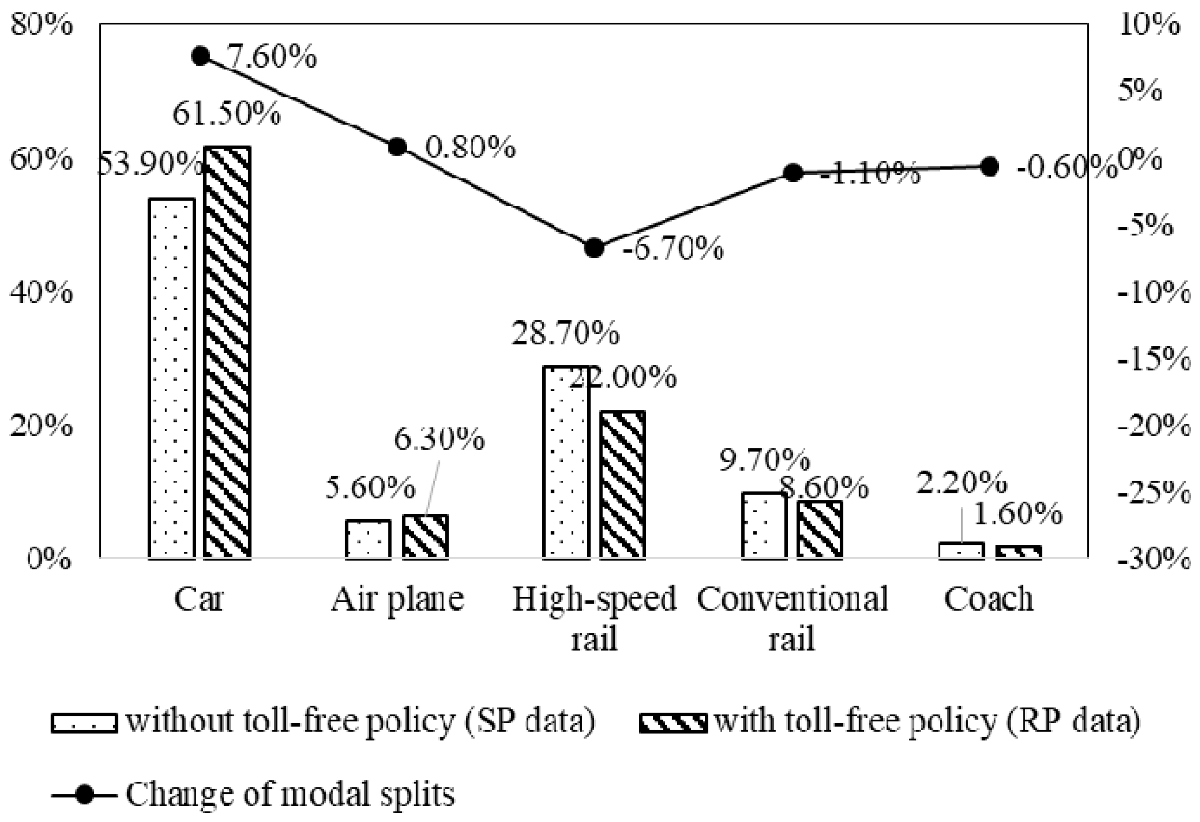
3.3. Descriptive Analysis

Figure 1 shows the modal splits for RP data with expressway toll-free policy and SP data without expressway toll-free policy. It is worth mentioning that SP an RP data consists of the same group of individuals. The car mode includes car driving and household carpooling. It reveals that car and HSR are the highest usage modes for intercity travel, which account for over 80% of the total demand. The comparison of these two datasets reveals that the elimination of road tolls has a vital impact on rising car usage and lower public transit demand. With the elimination of the road toll, the car share significantly increases from 53.9% to 61.5%. In terms of the modal splits of public transit, HSR is the most affected, whose share decreased from 28.7% to 22.0%. The total share of conventional rail and coach are both slightly affected by the elimination of road toll with a decrease of 1.1% and 0.6%. While almost all modal splits of public transit are decreased, there is a slight rise in the splits of the airplane, from 5.6% to 6.3%.

4. Model Specification

In this section, a mixed logit model is developed by assuming travelers choosing the following mode alternatives: car, airplane, HSR, conventional rail, and coach. Unlike urban traffic, intercity traffic mode systems are more independent and less affected by each other. We assume that there is no correlation between alternatives. In addition, as all respondents have made traffic mode choices repeatedly for outbound and inbound trips both in RP and SP scenarios, there is a correlation among repeated choice observations from a single respondent (panel effect). Hence, the mixed logit models are finally adapted to deal with the panel effects in the dataset.

Based on the theory of random utility maximization (McFadden D, 1974), decision-makers are assumed to be rational and to select the alternative with the highest utility among the available alternatives when making a choice. The utility function of choosing the mode $i$ by an individual $n\left(n=1,2,\cdots ,N\right)$ at the $t^{th}\left(t=1,2,\cdots ,T\right)$ number of scenarios consists of a systematic part $V_{\mathrm{int}}$ and an error term ${\epsilon }_{\mathrm{int}}$, which is given by:

$$\begin{array}{cc}{U}_{nit}=V_{nit}+{\epsilon }_{nit},& i\in C_n\end{array},$$

(1)

where $C_n$ is the available choice set for the individual $n$.

The systematic part $V_{nit}$, as shown in Equation (2), is a linear function of impact attributes $X_{nitk}$ and their marginal effect on utility ${\beta }_{ik}$, and an Alternative Specific Constant $AS{C}_i$ that captures systematic but unexplained variability in the data. In addition, the panel effect is captured by the normally distributed error component ${\eta }_{in}$ with zero mean and standard deviation ${\sigma }_i$.

$$V_{nit}=AS{C}_i+{\displaystyle \sum _{k=1}^{K_i}{\beta }_{ik}}{X}_{nitk}+{\sigma }_i{\eta }_{ni},$$

(2)

The probability of choosing the alternative $i$ at the $t^{th}\left(t=1,2,\cdots ,T\right)$ number of scenarios depends on the utility of the alternative $i$ and other alternatives $j$ in the available choice set $C_n$, as shown in Equation (3).

$$P_{nit}\left(\beta \right)=\frac{\exp \left(V_{nit}\left(\beta \right)\right)}{{\displaystyle {\sum }_{j=1}^{C_n}\exp \left(V_{njt}\left(\beta \right)\right)}},$$

(3)

To account for the panel effect, the probability of the sequence of choices $T=\left\{t|1,2,3,4,5,6\right\}$ from the same individual $n$ is estimated as in Equation (4):

$$P_{ni}\left(\beta \right)={\displaystyle \prod _{t=1}^T\frac{\exp \left(V_{nit}\left(\beta \right)\right)}{{\displaystyle {\sum }_{j=1}^{C_n}\exp \left(V_{njt}\left(\beta \right)\right)}}},$$

(4)

Finally, the mixed logit models with panel effects only, as in Equation (4), have been estimated.

The explanatory variables and parameter setting are listed in

Table 3. Explanatory Variables and Measurements.

Variable	Parameter Setting	Measurement
Socio-economic Factors
Male	Alternative specific for direct effects; Generic for interaction effects	1 if gender is male, 0 if female
Age		numeric variable
Car ownership		1 if household own at least one car, 0 if else
Lower income 1,2		1 if annual disposable income per capita in the household is under ¥40,000, 0 if else
Child		1 if there is at least a child (under 18 years old) in the household, 0 otherwise
Mode Attributes
Travel cost 2 (¥100)	Generic	road toll × toll-distance + fuel charge
Travel time (hour)	Generic	travel time by car = driving time; travel time by public transit = travel time in vehicle + transfer time out of vehicle + waiting time in the public transit station.
Evening-to-Morning Train (conventional rail only)	Alternative specific	1 if the train departing between 12:00–24:00 and arriving between 06:00–12:00 on the next day, 0 if else.

¹ the average annual disposable income per capita in the household is ¥40,000–50,000 in Beijing, 2017; ² ¥1 ≈ $0.15.

. The explanatory variables include socio-economic factors and mode attributes. Socio-economic factors consist of gender, age, household income, household car ownership, and living with children in the household. Their direct effects on mode choice utilities are treated as alternative specific variables. In addition, to differentiate the impact of policies among the population, their interaction effect with the travel cost (i.e., systematic taste heterogeneity) are tested. The systematic heterogeneity variables are set as generic variables. As for mode attributes, travel time and travel cost are set as generic variables. In consideration of the particularity of evening-to-morning trains, they are also included in the model as an alternative specific variable for the utility of choosing conventional rail.

To identify the correct explanatory variables, several MNL models without the panel error term in Equation (2) have been estimated preliminarily. First, for each variable, its impact on all mode choice utilities are measured and then the one which parameter value is closest to zero is identified as the reference item and then eliminated from the model. Second, the variable that displayed highest insignificant effect on mode choice utilities dropped out one by one to avoid type I errors (incorrect rejection of a true null hypothesis). Finally, the mixed logit model was estimated with parameters that are significant in the MNL model.

Three availability conditions were included in the model specification: (1) Any travelers going to a city where there is no airport within four hours driving was assumed not to have an airplane service; (2) Any travelers going to a city where there is no HSR station/conventional rail station within three hours driving was assumed not to have the high-speed rail/conventional rail service; (3) Any travelers going to a county where there is no coach station within two hours driving was assumed not to have the coach service. In consideration of the convenience of car rental nowadays, the car mode is available to all individuals no matter if his/her household own a car or not.

5. Results and Discussion

To estimate the mixed logit models, PythonBiogeme [46] was used.

Table 4. Model Information Report.

Number of draws	500
Number of estimated parameters	28
Number of observations	7260
Number of individuals	1815
Initial log-likelihood	−10,098
Final log-likelihood	−5410
Likelihood ratio test for the initial model	9376.571
Rho-square	0.464
Adjusted rho-square-bar	0.462

shows the model information report. All responses for outbound and inbound trips are treated equally and together in the model, including the RP responses with the expressway toll-free policy and the SP responses without the policy. In total, 7260 observations are used in the model estimation. As the models do not have a closed form, the probabilities $P_{ni}$ are approximated by simulation [47]. 500 draws were sampled for each observation in this study.

In principle, there are 37 parameters (4 ASC, 20 alternative specific parameters for socio-economic factors, 9 generic parameters for travel attributes and systematic taste heterogeneity, and 4 standard deviations for panel error term) that can be estimated given the model formulation and explanatory variables list presented in Table 3. However, many parameters turned out to be insignificant in the preliminary MNL model specification. Finally, 27 parameters were estimated in the mixed logit model. The parameter estimation results are presented in

Table 5. Estimated parameters of the Mixed Logit Model for Mode Change.

Variable	Coefficient Estimation	Std Err	t-Test	p-Value
Alternative Specific Constant
ASC (air)	−3.72	0.854	−4.36	0.00
ASC (HSR)	1.40	0.584	2.40	0.02
ASC (CR)	−0.753	1.180	−0.64	0.52	**
ASC (coach)	−1.07	0.571	−1.88	0.06	*
Socio-economic Factors
Male (air)	0.999	0.445	2.24	0.02
Male (HSR)	−1.29	0.278	−4.63	0.00
Male (CR)	−1.43	0.522	−2.74	0.01
Age (car)	0.0548	0.015	3.60	0.00
Age (CR)	−0.0868	0.034	−2.54	0.01
Lower Income (Car)	−0.775	0.276	−2.81	0.00
Lower Income (CR)	3.49	0.620	5.64	0.00
Lower Income (Coach)	0.720	0.344	2.09	0.04
Car Ownership (Car)	4.52	0.362	12.48	0.00
Car Ownership (Air)	1.86	0.460	4.03	0.00
Car ownership (CR)	−3.85	0.654	−5.89	0.00
Child (Car)	1.53	0.264	5.80	0.00
Child (Air)	0.893	0.416	2.15	0.03
Mode Attributes
Travel Cost (100 RMB)	−0.500	0.070	−7.16	0.00
Travel Time (Hour)	−0.533	0.032	−16.60	0.00
Evening-to-Morning Train (CR)	0.608	0.131	4.64	0.00
Systematic Taste Heterogeneity
Travel Cost * Lower Income	−0.0917	0.039	−2.37	0.02
Travel Cost * Male	−0.0821	0.044	−1.87	0.06	*
Panel Effect
SIGMA (Car)	−3.50	0.233	−15.02	0.00
SIGMA (Air)	3.07	0.481	6.37	0.00
SIGMA (HSR)	4.08	0.286	14.26	0.00
SIGMA (CR)	8.76	0.671	13.06	0.00

* Parameter values not meeting the 95% significance level; ** Parameter values not meeting the 90% significance level; HSR: high-speed rail; CR: conventional rail.

.

The model has a McFadden’s rho-square value of 0.462 and has a significantly higher explanatory power than the null model (Log-likelihood ratio for the final ML model (−5410) is larger than that for the initial zero beta model (−10,098)).

The estimated coefficient in Table 5 indicates the marginal change in the utility of choosing mode if the value of its corresponding variable increases by one unit. For example, the coefficient number for Male (air) in Table 5 denotes that men would increase the utility of individuals choosing airplane mode by 0.999 than women, with a significant t-statistic at 5% level.

In terms of mode characteristics, the travel cost and travel time have a significantly negative impact on the utilities. The result is in line with expectations. Moreover, the evening-to-morning train has a positive effect on the utility of conventional rail with significant t-statistic at 1% level. It indicates that people are more likely to take the evening-to-morning train than other kinds of conventional rail with different departure and arrival time arrangement. The result fits in with the literature result [40] which distinguished rail into day train and night train.

In the case of individual characteristics, men have a higher airplane use and lower rail (both HSR and conventional rail) use compared to women. Regarding individuals of different age, the elder, as expected, are more likely to use car mode in comparison with the youth. In addition, the elder is less likely to take conventional rail because it takes more time and is more exhausting. For household attributes, households with lower income have a lower usage of the car and higher usage of conventional rail and coach than households with higher income. In the contrast, households owning cars have a higher usage of car, airplane and lower usage of conventional rail than households without a car. It is reasonable because a household owning a car is more likely to have a higher income. Finally, adults living with children are more like to travel by car or by air.

5.1. Who Will Be More Sensitive in Changing Mode in Response to the Policy?

One of the interesting aspects of the study is who will change mode on account of the reduction in the road toll. To investigate this problem, the interaction effects between each socio-economic factor and the travel cost have been included in the model. Table 5 shows that the mode choice is significantly associated with the variables in male and lower income. The negative sign of these two interaction effects indicates that, compared to women and higher-income travelers, men and lower-income travelers are more sensitive to the cost and are furthermore likely to change mode in response to variation of road toll. Other individual attributes (age, car ownership, living with children in the household) are also analyzed by way of systematic taste heterogeneity. However, the results are not included in the final models due to insignificance.

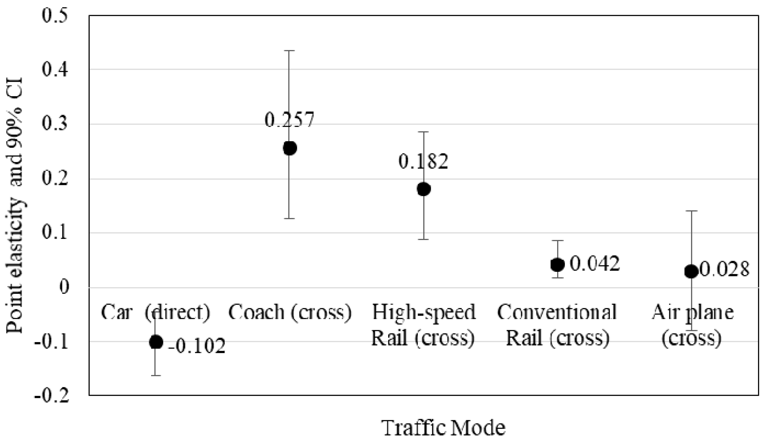
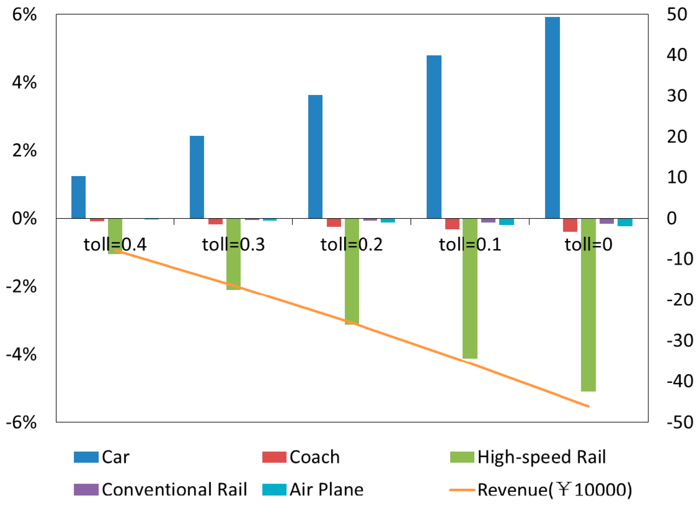
5.2. To What Extent Would a Decrease in Road Toll Suppress Demand of Each Public Transit Mode?

The other objective of this study is to find out to what extent the ridership of different public transit modes can be expected to be suppressed because of the decrease in the road toll. The elasticities are widely used to anticipate the impact of a change of the variable value on the choice of individuals. Thus, the objective was explored by comparing the direct/cross-elasticity of each mode with respect to the road toll, as shown in Figure 2. It shows that a 1% increase of the road toll has a negative impact on the choice probability of car driving, and have a positive influence on the choice probability of public transit modes. Analogously, it confirms that the decrease of road toll has a positive effect on encouraging travelers to change their travel mode from public transit to private car driving.

Road toll affects public transit modes probabilities in a different way. By comparing the cross-elasticity values, the order of how much the public transit riders will be affected by the reduction of the road toll, from the most to the least sensitive, is coach, HSR, conventional rail, and airplane. With larger elasticities for coach and HSR than for conventional rail and airplane choice, it shows coach and HSR travelers are more sensitive to road toll change than conventional rail and airplane riders. It reveals that car driving is a better substitute for the coach and HSR. By contrast, air transport users are the most insensitive group to the policy because they usually travel longer distances, place a higher value of time and have a lower sensitivity to cost in general. In addition, it is interesting that HSR and conventional rail are similar modes but represent quite different sensitiveness to the road toll. It unveiled that there is clear product differentiation between HSR and conventional rail, which raises the need to differentiate them in mode choice modeling for long-distance travel.

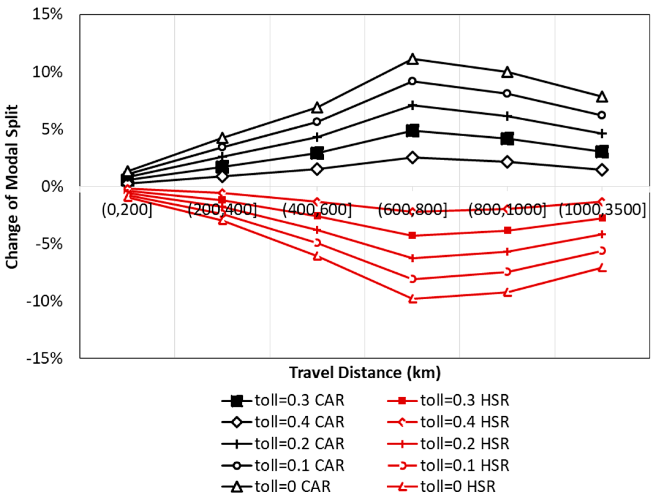
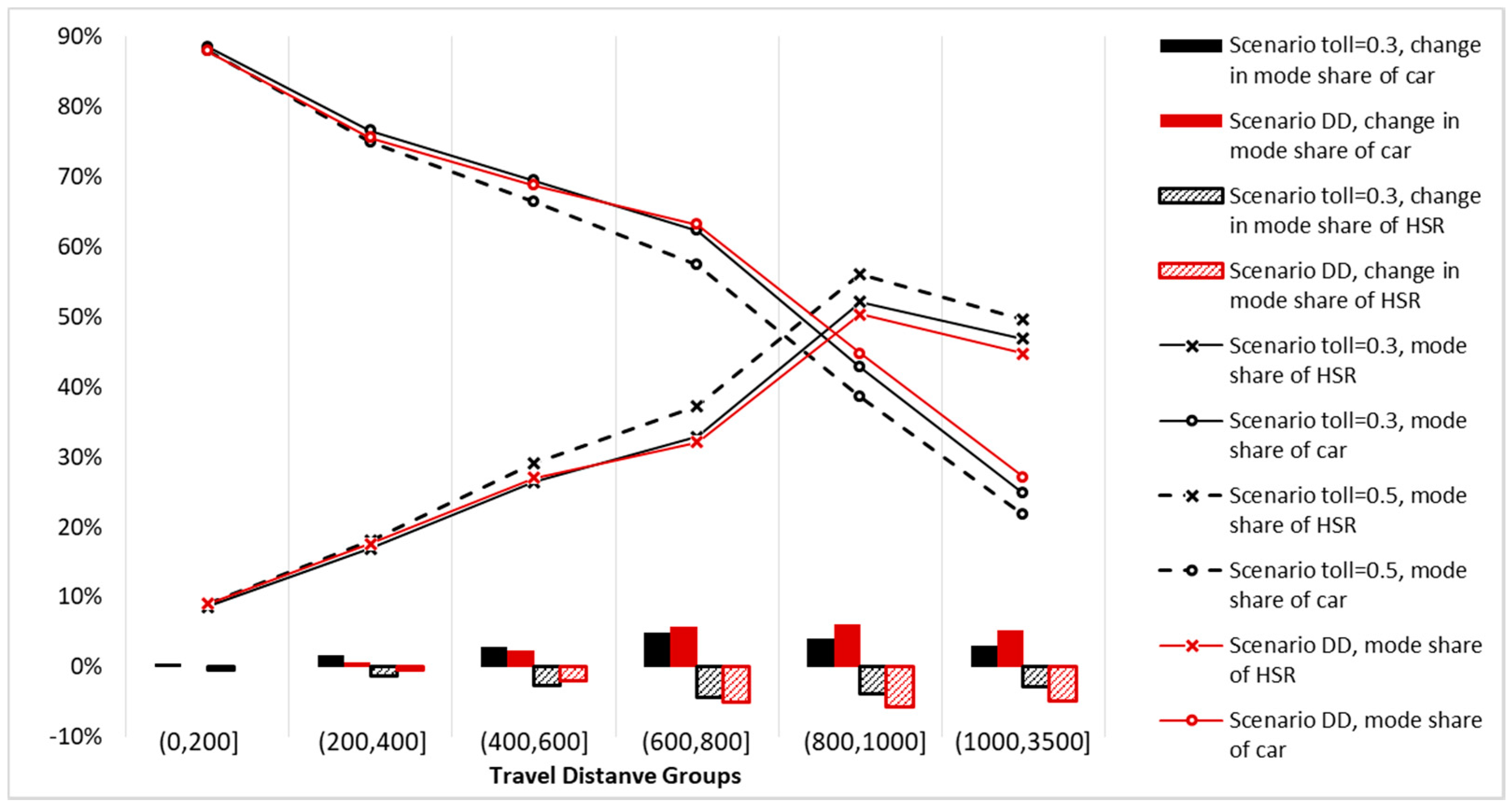
5.3. Policy Impact Analysis on Travel Distance

Several scenarios are proposed to help explore the effectiveness of different policy options aiming at decreasing public transit congestion during the holiday period. Scenarios D0–D5 are proposed to compare policy effectiveness with distinct toll discounts. The modal splits and revenues in each scenario are simulated by sample enumeration based on the model estimation results. The revenue here only refers to the total road toll for car usage, but does not include fares of public transit.

Table 6. Scenarios and Modal Splits of Total Population.

Scenarios (¥1 ≈ $0.15)
D0	Road toll = ¥0.5/km, Baseline
D1	Road toll = ¥0.4/km
D2	Road toll = ¥0.3/km
D3	Road toll = ¥0.2/km
D4	Road toll = ¥0.1/km
D5	Road toll = ¥0/km
DD	Road toll = ¥0.5/km for tolling distance within 200 km (200 km included); road toll = ¥0.3/km for tolling distance within 200–400 km (400 km included); road toll = ¥0.1/km for tolling distance within 400–600 km (600 km included); road toll is free for tolling distance over 600 km.
Modal Splits
	Car	Coach	HSR 1	CR 2	Air	Revenue (¥10,000)
D0 (baseline)	59.74%	1.76%	29.61%	3.03%	5.86%	46.1213
D1	60.96%	1.67%	28.55%	3.01%	5.82%	38.1986
D2	62.16%	1.58%	27.50%	2.98%	5.78%	29.6422
D3	63.35%	1.50%	26.48%	2.95%	5.73%	20.4253
D4	64.52%	1.42%	25.48%	2.91%	5.67%	10.5425
D5	65.66%	1.34%	24.50%	2.87%	5.62%	0
DD	62.52%	1.65%	27.11%	3.01%	5.72%	28.8790

¹ HSR: high-speed rail; ² CR: conventional rail.

shows the simulation results. The modal splits of the scenario D0 are taken as the baseline because the road toll in this scenario (¥0.5/km) equals the general toll in China during the workday in 2017. Changes of modal splits with different toll discounts are shown in Figure 3 (D0–D5). It shows that cheaper road tolls can indeed improve the demand for car driving, meanwhile the demand for public transit usage drops. The increases in car driving demand largely come from the shrinking demand for HSR, rather than coach, airplane, and conventional rail. Although the coach riders are the most sensitive to the policy, the original coach ridership is too little to lead to a sizable decrease in coach share. In total, simulation results agree well with the foregoing elasticity analysis result in Section 3.1.

In addition, it is well known that travel distance strongly impacts people’s propensities to mode choice. The modal splits are then quite different in response to the variation in trip distance. It might be that people also react differently to a certain policy measures when traveling different distances. In this case, a certain policy measure has a different effect for people with different travel distances. To explore the phenomenon, the survey dataset is divided into six distance groups. For each distance group, the modal splits in each scenario are also simulated. Take the scenario D0 as the reference, changes of modal splits of the car and HSR for each distance group in other scenarios are shown in Figure 4. It is easily noticed that the effectiveness of policy is firstly increasing and then decreasing in response to the distance increase. The effect on choice probability by variations in road toll can be considered as negligible for alternatives within 200 km travel distance, and this effect is greatest for alternatives between 600 and 800 km travel distance. Such a finding presents the same trend in the aforementioned study for intercity travel [37]. In fact, the result is also similar to the results of the previous literature for urban commute travel [16].

Inspired by the policy effectiveness change in response to the variation in trip distance, a distance-based discount measurement is considered. As described in the introduction section, although the modal transfer from public transit to car driving can decreasing public transit congestion during the holiday period, it may also lead to the side effect of aggravating congestion delays on expressway networks and increasing air pollution. Therefore, a trade-off between the policy objective and the side effect is important. Since the car accounts for a higher share in short-distance trips and HSR accounts for a larger proportion of medium- and longer-distance trips, traffic managers may want to restrain the modal transfer from HSR to the car for short-distance trips and encourage it for long-distance trips. In this case, to give less toll discount for short-distance trips and more toll discount for long-distance trips might be helpful. Hence, a distance-based discount scenario is proposed, which is denoted as scenario DD in Table 6. In this scenario, no discount is given for trips within 200 km, 40% discount is given for trips within 200–400 km, 80% discount is given for trips within 400–600 km, and all road toll is eliminated for trips distance over 600 km.

The modal splits for each distance group in scenario DD are compared to that in scenario D2 because the total change in car share and revenues of these two scenarios are the most similar. The comparison result is shown in Figure 5. It verifies that the distance-based discount policy can restrain the short-distance transportation mode transfer from HSR to the car mode (distance group 1–3 in Figure 5), promote the long-distance travel mode transfer (distance group 4–6 in Figure 5), and pertinently alleviate the high incidence regions with higher HSR demand. It is more targeted and more effective than the indiscriminate discount policy.

6. Conclusions

Using the RP and SP survey data from the 2017 Spring Festival Holiday in China, a mixed logit model is estimated to model intercity mode choice behavior. Based on the model estimation result, the implication of reducing road toll on mode choice behavior for intercity trips are investigated by three key questions. The common social-economic characteristics that are significantly associated with road tolls are identified, the influence extent of the toll discount policy on different public transit modes are compared, and the policy effectiveness variation by travel distance is explored.

The result shows that the reduction of road tolls is an efficient way to decrease public transit ridership and alleviate the problem of over-loaded public transit during the holiday period. First, men and lower-income travelers are identified to be more sensitive to travel cost and further be more likely to change mode in response to variation of road toll. Second, the order of how much the public transit riders will be affected by the reduction of the road toll, from the most to the least sensitive, is: coach, HSR, conventional rail, and airplane. Taking the initial mode share into account, the increases in car driving demand largely come from the shrinking demand for HSR, rather than coach, airplane, and conventional rail. Finally, the propensity to change mode in response to the road toll reduction (effectiveness of policy) is firstly increasing and then decreasing in response to the distance increase. Based on that, the distance-based discount policy is recommended because it is more targeted and more effective than the indiscriminate discount policy. It achieves the intended result by restraining the mode transfers for short-distance travel from HSR to cars, but promoting the mode transfer for long-distance travel, and so pertinently alleviating the high incidence regions with higher HSR demand.

Conclusions drawn from this article can still provide useful guidance on road pricing management. These observations suggest that policy coordination regarding toll levels is needed to avoid side effects on increased expressway congestion caused by toll-free policy. Moreover, compared to the indiscriminate discount policy on road tolling, differentiation policy regarding distance-based discounts is recommended and is worth studying to improve the pertinence and effectiveness of the policy. However, this study is based on survey data in Beijing from the 2017 Spring Festival. The results may be generalized to other specific holidays, such as Golden Week, whose travel purpose is tourism rather than visiting relatives. Further research can investigate other special holidays to conduct a more systematic analysis of the issue.

References

1. Nakamura, H. Holiday traffic activities and problems on planning procedure for recreational roads in Japan. IATSS Res. 1994, 18, 53–63. [Google Scholar]
2. Yai, T.; Yamada, H.; Okamoto, N. Nationwide recreation travel survey in Japan: Outline and modeling applicability. Transp. Res. Rec. 1995, 1493, 29–38. [Google Scholar]
3. Arnold, R.; Cerrelli, E.C. Holiday Effect on Traffic Fatalities; United States National Highway Traffic Safety Administration: Washington, DC, USA, 1987.
4. Emmel, P. Missouri Holiday Crashes Report; Missouri State Highway Patrol Statistical Analysis Center: Jefferson City, MO, USA, 2004.
5. Bell, T.J. Holiday roads: Stay safe this season. Traffic Saf. 2001, 1, 8–11. [Google Scholar]
6. Liu, C.; Chen, C.L. Time Series Analysis and Forecast of Crash Fatalities during Six Holiday Periods; Transportation Research Board: Washington, DC, USA, 2004. [Google Scholar]
7. Anowar, S.; Yasmin, S.; Tay, R. Comparison of crashes during public holidays and regular weekends. Accid. Anal. Prev. 2013, 51, 93–97. [Google Scholar] [CrossRef] [PubMed]
8. IEDAH. Historic Toll-Discount in Japan’s Intercity Expressway for Economic Stimulation: Its Four Aspects, Results, and Points at Issue. In Proceedings of the 8th International Conference of Eastern Asia Society for Transportation Studies, Kota, Indonesia, 16–19 November 2009; Volume 7, p. 75. [Google Scholar]
9. Takahashi, H.; Kameoka, H.; Mabuchi, K.; Sato, H.; Xing, J. Examining effects of TDM with toll discount on mitigation of expressway traffic congestion. In Proceedings of the 7th International Conference of Eastern Asia Society for Transportation Studies, Dalian, China, 24–27 September 2007; p. 76. [Google Scholar]
10. Fu, S.; Gu, Y. Highway toll and air pollution: Evidence from Chinese cities. J. Environ. Econ. Manag. 2017, 83, 32–49. [Google Scholar] [CrossRef]
11. Ying, J.; Ando, R. On the effects of central Japan expressway’s commuter toll discount policy in nagoya area. Tsinghua Sci. Technol. 2007, 12, 151–157. [Google Scholar] [CrossRef]
12. Bao, Y.; Xiao, F.; Gao, Z.; Gao, Z. Investigation of the traffic congestion during public holiday and the impact of the toll-exemption policy. Transp. Res. Part B Methodol. 2017, 104, 58–81. [Google Scholar] [CrossRef]
13. Steiner, T.J.; Bristow, A.L. Road pricing in National Parks: A case study in the Yorkshire Dales National Park. Transp. Policy 2000, 7, 93–103. [Google Scholar] [CrossRef]
14. Albert, G.; Mahalel, D. Congestion tolls and parking fees: A comparison of the potential effect on travel behavior. Transp. Policy 2006, 13, 496–502. [Google Scholar] [CrossRef]
15. Eliasson, J.; Mattsson, L.G. Equity effects of congestion pricing: Quantitative methodology and a case study for Stockholm. Transp. Res. Part A Policy Pract. 2006, 40, 602–620. [Google Scholar] [CrossRef]
16. Yang, L.; Zheng, G.; Zhu, X. Cross-nested logit model for the joint choice of residential location, travel mode, and departure time. Habitat Int. 2013, 38, 157–166. [Google Scholar] [CrossRef]
17. Moeckel, R.; Fussell, R.; Donnelly, R. Mode choice modeling for long-distance travel. Transp. Lett. 2015, 7, 35–46. [Google Scholar] [CrossRef]
18. Yan, X.Y.; Wang, W.X.; Gao, Z.Y.; Lai, Y.C. Universal model of individual and population mobility on diverse spatial scales. Nat. Commun. 2017, 8, 1639. [Google Scholar] [CrossRef] [PubMed] [Green Version]
19. Gordon, I.R.; Edwards, S.L. Holiday trip generation. J. Transp. Econ. Policy 1973, 7, 153–168. [Google Scholar]
20. Bureau of Transportation Statistics. America on the Go. US Holiday Travel; US Department of Transportation: Washington, DC, USA, 2003.
21. Axhausen, K.W. Methodological Research for a European Survey of Long-Distance Travel; Transportation Research E-circular Number E-C026; Transportation Research Board: Washington, DC, USA, 2001. [Google Scholar]
22. Böhler, S.; Grischkat, S.; Haustein, S.; Hunecke, M. Encouraging environmentally sustainable holiday travel. Transp. Res. Part A Policy Pract. 2006, 40, 652–670. [Google Scholar] [CrossRef]
23. Dickinson, J.E.; Robbins, D.; Lumsdon, L. Holiday travel discourses and climate change. J. Transp. Geogr. 2010, 18, 482–489. [Google Scholar] [CrossRef]
24. Zhang, L.; Southworth, F.; Xiong, C.; Sonnenberg, A. Methodological options and data sources for the development of long-distance passenger travel demand models: A comprehensive review. Transp. Rev. 2012, 32, 399–433. [Google Scholar] [CrossRef]
25. Ben-Akiva, M.E.; Lerman, S.R.; Lerman, S.R. Discrete Choice Analysis: Theory and Application to Travel Demand; MIT Press: Cambridge, MA, USA, 1985. [Google Scholar]
26. Train, K.E. Discrete Choice Methods with Simulation; Cambridge University Press: Cambridge, UK, 2009. [Google Scholar]
27. Langbroek, J.H.M.; Franklin, J.P.; Susilo, Y.O. The effect of policy incentives on electric vehicle adoption. Energy Policy 2016, 94, 94–103. [Google Scholar] [CrossRef]
28. Liu, C.; Wang, Q.; Susilo, Y.O. Assessing the impacts of collection-delivery points to individual’s activity-travel patterns: A greener last mile alternative? Transp. Res. Part E Logist. Transp. Rev. 2017. [Google Scholar] [CrossRef]
29. Li, W.; Kamargianni, M. Providing quantified evidence to policy makers for promoting bike-sharing in heavily air-polluted cities: A mode choice model and policy simulation for Taiyuan-China. Transp. Res. Part A Policy Pract. 2018, 111, 277–291. [Google Scholar] [CrossRef]
30. Wang, Y.; Yan, X.; Zhou, Y.; Xue, Q. Influencing mechanism of potential factors on passengers’ long-distance travel mode choices based on structural equation modeling. Sustainability 2017, 9, 1943. [Google Scholar] [CrossRef]
31. Wang, K.; Xia, W.; Zhang, A.; Zhang, Q. Effects of train speed on airline demand and price: Theory and empirical evidence from a natural experiment. Transp. Res. Part B Methodol. 2018, 114, 99–130. [Google Scholar] [CrossRef]
32. Givoni, M. Development and impact of the modern high-speed train: A review. Transp. Rev. 2006, 26, 593–611. [Google Scholar] [CrossRef]
33. Nuzzolo, A.; Crisalli, U.; Gangemi, F. A behavioral choice model for the evaluation of railway supply and pricing policies. Transp. Res. Part A Policy Pract. 2000, 34, 395–404. [Google Scholar] [CrossRef]
34. Yao, E.; Morikawa, T. A study of on integrated intercity travel demand model. Transp. Res. Part A Policy Pract. 2005, 39, 367–381. [Google Scholar] [CrossRef]
35. Mandel, B.; Gaudry, M.; Rothengatter, W. A disaggregate Box-Cox Logit mode choice model of intercity passenger travel in Germany and its implications for high-speed rail demand forecasts. Ann. Reg. Sci. 1997, 31, 99–120. [Google Scholar] [CrossRef]
36. Forinash, C.V.; Koppelman, F.S. Application and interpretation of nested logit models of intercity mode choice. Transp. Res. Rec. 1993, 1413, 98–106. [Google Scholar]
37. Lin, X.M.; Shao, C.F.; Qian, J.P.; Zhang, Y.D. Evolution dynamic of the expressway toll-free policy impact on the mode choice in a bimodal transportation network during holidays. Adv. Mech. Eng. 2017, 9. [Google Scholar] [CrossRef]
38. Bhat, C.R. A heteroscedastic extreme value model of intercity travel mode choice. Transp. Res. Part B Methodol. 1995, 29, 471–483. [Google Scholar] [CrossRef]
39. Bhat, C.R. An endogenous segmentation mode choice model with an application to intercity travel. Transp. Sci. 1997, 31, 34–48. [Google Scholar] [CrossRef]
40. Monzon, A.; Rodríguez-Dapena, A. Choice of mode of transport for long-distance trips: Solving the problem of sparse data. Transp. Res. Part A Policy Pract. 2006, 40, 587–601. [Google Scholar] [CrossRef]
41. Fu, X.; Oum, T.H.; Yan, J. An analysis of travel demand in Japan’s intercity market empirical estimation and policy simulation. J. Transp. Econ. Policy 2014, 48, 97–113. [Google Scholar]
42. Limtanakool, N.; Dijst, M.; Schwanen, T. The influence of socioeconomic characteristics, land use and travel time considerations on mode choice for medium-and longer-distance trips. J. Transp. Geogr. 2006, 14, 327–341. [Google Scholar] [CrossRef]
43. Srinivasan, S.; Bhat, C.R.; Holguin-Veras, J. Empirical analysis of the impact of security perception on intercity mode choice: A panel rank-ordered mixed logit model. Transp. Res. Rec. 2006, 1942, 9–15. [Google Scholar] [CrossRef]
44. LaMondia, J.; Snell, T.; Bhat, C.R. Traveler behavior and values analysis in the context of vacation destination and travel mode choices: European Union case study. Transp. Res. Rec. 2010, 2156, 140–149. [Google Scholar] [CrossRef]
45. Rojo, M.; Gonzalo-Orden, H.; dell’Olio, L.; Ibeas, A. Relationship between service quality and demand for inter-urban buses. Transp. Res. Part A Policy Pract. 2012, 46, 1716–1729. [Google Scholar] [CrossRef]
46. Bierlaire, M. PythonBiogeme: A Short Introduction; Series on Biogeme; Transport and Mobility Laboratory, School of Architecture, Civil and Environmental Engineering, Ecole Polytechnique Fédérale de Lausanne: Lausanne, Switzerland, 2016. [Google Scholar]
47. Bhat, C.R. Simulation estimation of mixed discrete choice models using randomized and scrambled Halton sequences. Transp. Res. Part B Methodol. 2003, 37, 837–855. [Google Scholar] [CrossRef] [Green Version]
Figure 1. Modal Splits of the Sample.
Sustainability 10 02700 g001
Figure 2. Direct and cross point elasticity in response to increasing road toll.
Sustainability 10 02700 g002
Figure 3. Change of modal splits with different toll discounts.
Sustainability 10 02700 g003
Figure 4. Change of modal splits by distance groups with different toll discounts.
Sustainability 10 02700 g004
Figure 5. Change of modal splits for each distance groups in scenarios DD and D2.
Sustainability 10 02700 g005