Substructure Hybrid Simulation Boundary Technique Based on Beam/Column Inflection Points


1
Department of Civil Engineering, Harbin Institute of Technology at Weihai, Weihai 264209, China
2
College of Civil Engineering, Fuzhou University, Fuzhou 350116, China
3
Department of Civil Engineering, Southeast University, Nanjing 210096, China
4
Department of Civil and Environmental Engineering, University of Illinois at Urbana-Champaign, Urbana, IL 61801, USA
*
Authors to whom correspondence should be addressed.
Sustainability 2018, 10(8), 2655; https://doi.org/10.3390/su10082655
Submission received: 2 July 2018
/
Revised: 24 July 2018
/
Accepted: 26 July 2018
/
Published: 28 July 2018
(This article belongs to the Special Issue Resilience and Sustainability of Civil Infrastructures under Extreme Loads)
Abstract
:Compatibility among substructures is an issue for hybrid simulation. Traditionally, the structure model is regarded as the idealized shear model. The equilibrium and compatibility of the axial and rotational direction at the substructure boundary are neglected. To improve the traditional boundary technique, this paper presents a novel substructure hybrid simulation boundary technique based on beam/column inflection points, which can effectively avoid the complex operation for realizing the bending moment at the boundary by using the features of the inflection point where the bending moment need not be simulated in the physical substructure. An axial displacement prediction technique and the equivalent force control method are used to realize the proposed method. The numerical simulation test scheme for the different boundary techniques was designed to consider three factors: (i) the different structural layers; (ii) the line stiffness ratio of the beam to column; and (iii) the peak acceleration. The simulation results for a variety of numerical tests show that the proposed technique shows better performance than the traditional technique, demonstrating its potential in improving HS test accuracy. Finally, the accuracy and feasibility of the proposed boundary technique is verified experimentally through the substructure hybrid simulation tests of a six-story steel frame model.
1. Introduction
Hybrid simulation (HS), also known as pseudo-dynamic testing, was initially proposed in 1969 [1]. This approach [2,3,4], which is a combination of physical testing and numerical simulation, has been widely used to evaluate the seismic performance of a structure, because it is efficient and cost-effective. HS takes the critical parts of a structure, which cannot be simulated adequately with the numerical simulation, as the physical substructure to test in the lab. The rest of the structure is taken as the numerical substructure and simulated using appropriate finite element software. Simulation of the laboratory and computer parts of the structure are carried out simultaneously, exchanging information about the responses at the boundary at each time step. Furthermore, the HS method transforms a real-time dynamic test under earthquake loads into a static loading test by simulating the dynamic components of the structural response in the computer, thus reducing the requirement for the loading devices and making large-scale or even full-scale model tests possible.
Initial research on the HS was overwhelmingly focused in Japan and the United States. Beginning in the 1990s, development and application of HS in Europe, Asia, and other regions grew significantly [5,6,7]. For structural systems with rate-dependent components, real-time HS testing was proposed and developed [8,9,10,11,12,13,14,15]. Moreover, HS also allows testing to be geographically distributed in multiple testing facilities. Many countries have been begun to build networked structures laboratories and developed a variety of HS platforms [16,17,18,19] to allow performance assessment of modern building structure systems. The largest is the Network for Earthquake Engineering Simulation (NEES) supported by the United States National Science Foundation from 1999 to 2014 [20,21,22,23]. NEES featured 14 geographically distributed and shared-use laboratories to test modern structural system.
Although substantial advances have been made in HS, achieving equilibrium and compatibility of the boundaries between the two substructures remains problematic, possibly limiting the accuracy of HS tests. There are currently four Multi-Axis Substructure Testing MAST systems in the world including MAST at the University of Illinois at Urbana-Champaign (UIUC), the University of Minnesota (USA), Swinburne University of Technology (Australia) and Ecole Polytechnique Montreal (Canada) that have the capabilities of six-DOF switched and mixed displacement and force modes of control [24,25,26]. The MAST at Swinburne has already been used in such hybrid simulation tests. However, controlling and measuring the force and displacement in all DOF is challenging. The method we present is relatively simple and can be widely implemented.
The fact that it cannot consider the effect of bending moments has always been a flaw for the HS method. However, this method has also been widely used in various structures due to its effectiveness, not just limited to shear buildings, as described in the literature [27,28,29,30,31,32,33,34,35]. In these tests, the conventional method of placing the loading position at each layer was widely adopted without considering the effect of the bending moment.
This paper proposes and improves a novel boundary technique based on a beam’s inflection point that can avoid the complex operation for realizing bending moments at the substructure boundary, based on previous a series of experimental techniques [34,36,37]. Following a description of the proposed boundary condition technique, a discussion of various implementation challenges is presented. The proposed method was validated through virtual HS, and experimental validation was carried out using a six-story steel frame model. The results demonstrate the efficacy of the proposed approach.
2. Boundary Technique for the HS
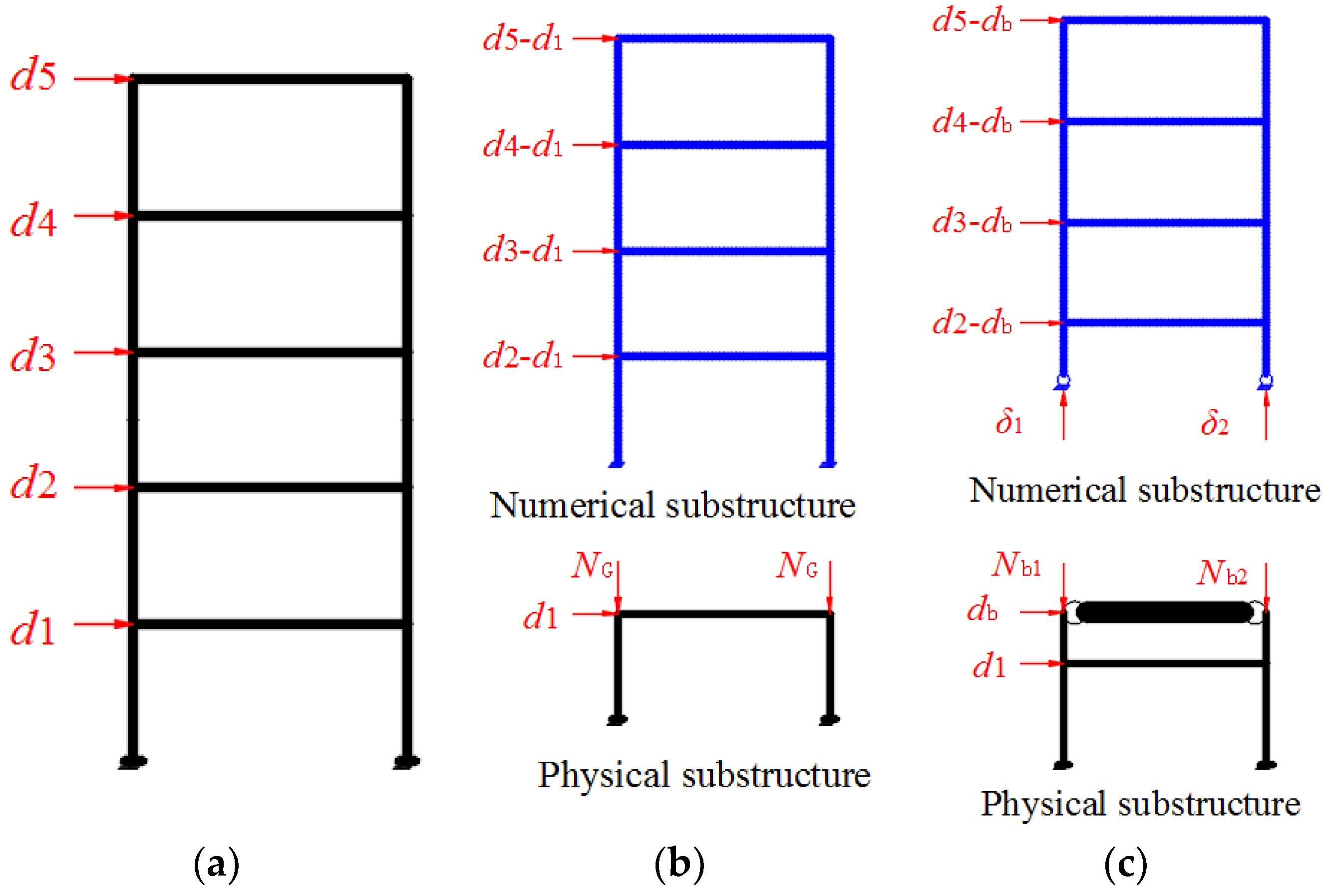
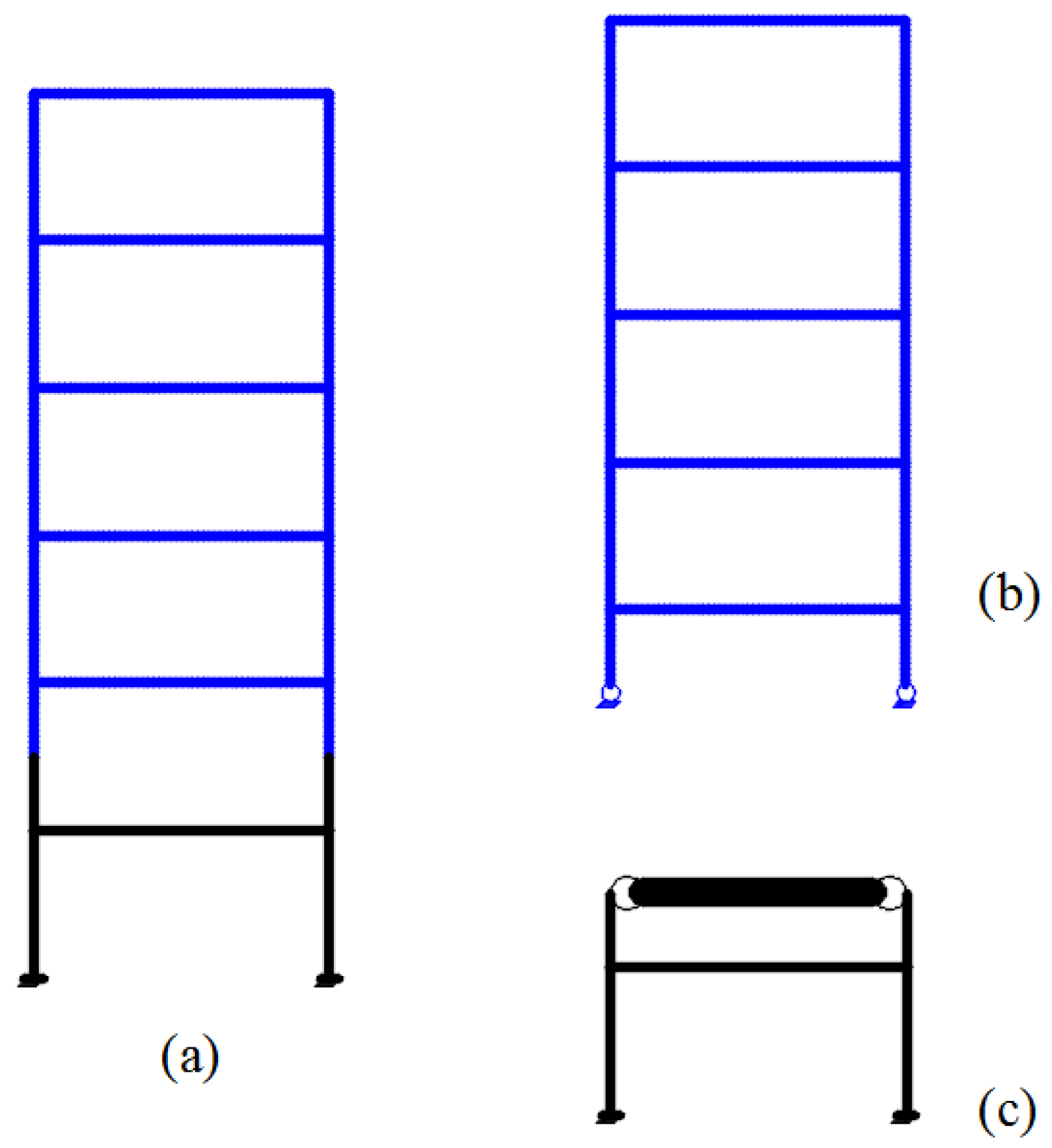
The compatibility and equilibrium conditions should be satisfied at the boundary between the physical and the numerical substructures during the HS. Consider the five-story example shown in Figure 1. Figure 1a shows the full model of the structure. Figure 1b illustrates the traditional boundary between two substructures, which is located at the top of the first story. This traditional boundary strategy mainly takes the structure model as an idealized shear model. The equilibrium of shear forces and the compatibility of the horizontal or shear displacement is satisfied by the hydraulic actuator. The equilibrium of the bending moment and axial force, as well as the compatibility axial and rotational deformations are typically neglected. Consequently, only two kinds of loading device are required at the boundary between the numerical substructure and the physical substructure: (i) one is the horizontal loading device to impose the shear force or displacement; and (ii) the other is the vertical loading device to simulate the gravity load due to upper stories, which is usually taken to be constant during the test. Therefore, several inevitable errors are introduced by not satisfying compatibility and equilibrium conditions.
To meet the equilibrium and compatibility in the axial and rotational direction at the boundary, more than two hydraulic actuators are required, as well as appropriate sensors to measure the rotational angle and the axial deflection, which can be challenging. To address the problems, a new boundary technique based on the inflection point is proposed, as shown in Figure 1c. The bending moments at the section of the inflection point in a structure is zero; therefore, this new boundary technique can effectively avoid the complex operation for realizing the bending moment at the boundary. However, two new problems arise in the proposed boundary technique: (i) how to calculate the horizontal displacement of the inflection point; and (ii) how to meet equilibrium and compatibility in the axial direction.
For the first problem, assuming a uniform column between two floors, then the displacement with respect to the lower floor at the inflection point is a linear interpolation value of the interstory drift for the corresponding floor. Adding a new concentrated mass or a degree of freedom (DOF) on the inflection point of each story is the direct method to solve the first problem for the proposed boundary technique. However, the DOF of the equation of motion (EOM) will increase significantly so that the stability and efficiency of the HS is influenced. A linear interpolation technique is used to determine the displacement at the inflection point. The calculated displacement at the inflection point is from the interstory drift of the corresponding floor. Therefore, the solution of the EOM is not different from the traditional method.
For the second problem, the axial displacement prediction technique at the boundary is presented, because the axial displacement is usually too small to measure accurately using displacement sensors [25]. Moreover, the axial displacement at the boundary must be obtained to start the simulation of the numerical substructure for the next step, so that the axial forces can be obtained from the numerical substructure simulation results to apply to the boundary of the physical substructure by the hydraulic actuators. Traditionally, an iteration strategy should be introduced to calculate the axial displacement. However, such iteration strategies will result in inevitable measure errors, because the physical substructure will be loaded many times during the iteration. To avoid iteration, an axial displacement prediction technique is presented to predict the axial displacement using the loading axial force, the assumption of the elastic axial deformation during the test, and the equilibrium equation.
The proposed prediction method is given by the following equation
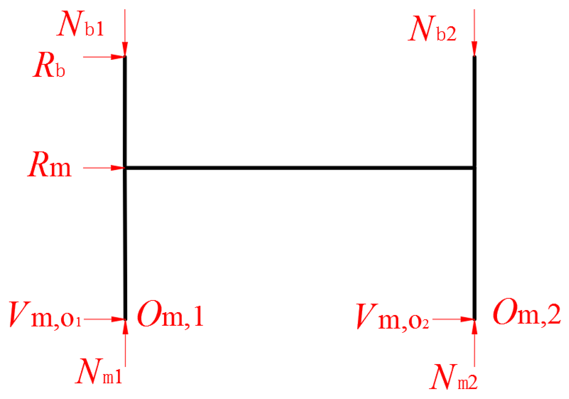
in which is the prediction axial deformation at the step i; m is the number of stories in the physical substructure; is the calculated axial force of the j-story at the step i; is the calculated axial force of the boundary story, which is calculated from the numerical substructure; is the height of the j-story of the physical substructure; is the height from the inflection point to the floor of the boundary story; is the axial stiffness of the jth-story of the physical substructure, which is constant during the test due to the assumption of the elastic axial deformation; and is the axial stiffness of the boundary story of the physical substructure. Here, can be calculated by the equilibrium equation. For example, consider the top story of the physical substructure shown in Figure 2. Here, L is the span of the frame; point Om,1 and Om,2 are inflection points of the m story; hI,m is the height from the inflection point to the roof of the m story; is the applied force by the actuator at the boundary; and is the applied force by the actuator at the mth-story. Noting that the dynamics of the frame are represented in the computer and using the moment equilibrium equation, the axial force can be calculated by taking moments about point O1 or O2. In the same way, the axial force of each story of the physical substructure can be calculated from the results of the upper story. Then, the axial forces of the physical substructure can be obtained. Subsequently, the prediction axial displacement at the boundary can be calculated using Equation (1), i.e.,
3. Implement of Boundary Technique
3.1. HS Component Interaction
Typically, the HS test includes three main components: the physical substructure, the numerical substructure, and the numerical integration routine. Early HS tests usually used an idealized mass-spring-damper model whose performance is known a priori to simulate the numerical substructure, allowing the software controlling the entire HS test to be realized as in a single program (e.g., written in FORTRAN or C). As HS testing has developed, researchers have sought to use more and more complicated models, in terms of both experimental and computational components. Computational components tailored for a particular strength are combined with general purpose finite element programs to achieve more accurate simulation. For example, a high-fidelity ABAQUS model was used [38], combined with the Matlab-based UI-SimCor [17], to investigate the seismic performance of semirigid steel joints. To address current research needs, HS testing software must accommodate different computational components.
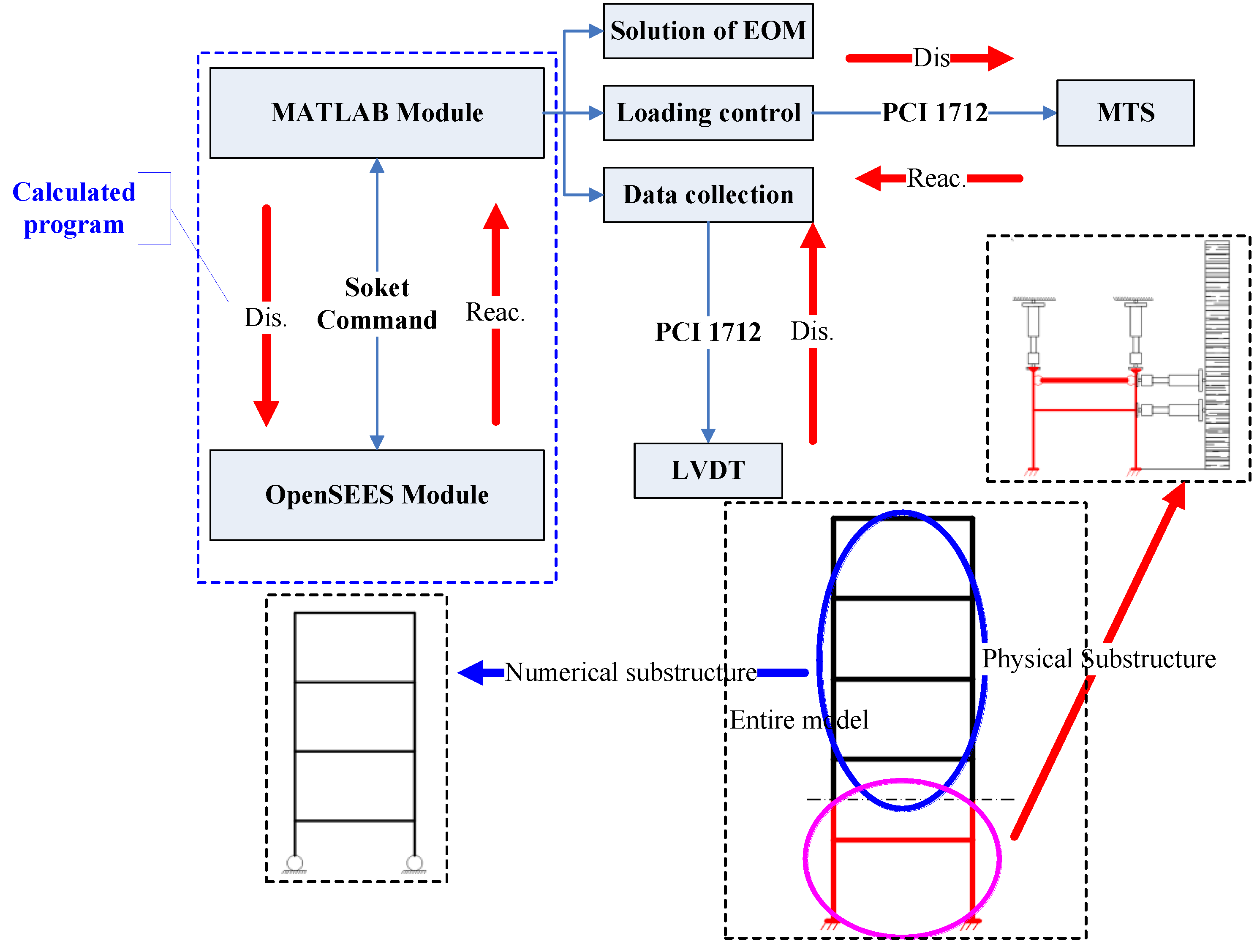
Communication between the computational and experimental components must be considered to realize a HS test. Figure 3 shows the sketch of the HS component interaction. First, OpenSEES is used to simulate both the physical and the numerical substructure in the virtual HS test, while MATLAB is employed to integrate the EOM. To realize the required data transfer, a communication bridge between the two different computational components is constructed. Data communication will take place at each step; each independent unit writes data to the other units and waits for the data written by other units. Moreover, the waiting or calculating time at different step is not uniform. This paper employs the network socket technique as a bridge to communicate the data between the two different computational components. In the MATLAB component, the TCPIP and ECHOTCPIP commands are used to construct an ICPIP object associated with OpenSEES. Concurrently, the command SOCKET in OpenSEES program is used to communicate with the Matlab program. Subsequently, a data acquisition card of PCI 1712 manufactured by the Advantech is employed as the communication bridge between the MATLAB and the MTS loading device. The PCI-1712 card provides a total of 16 single-ended or eight differential A/D input channels or a mixed combination, two 12-bit D/A output channels, 16 digital input/output channels, and three 10 MHz 16-bit multifunction counter channels.
3.2. Equivalent Force Control Method
Research on various integration algorithms employed for HS testing is very active. For example, the CR and KR-α methods [10,35] which have unconditional stability for linear elastic and stiffness softening nonlinear systems, were presented. However, the implicit algorithms generally require iteration, which can result in inconsistent HS test results. To avoid iteration, an equivalent force control (EFC) method [39], which uses feedback control to replace numerical iteration for the real-time HS testing, was proposed. EFC method was used to a full-scale six-story frame-supported reinforced concrete masonry shear wall [39].
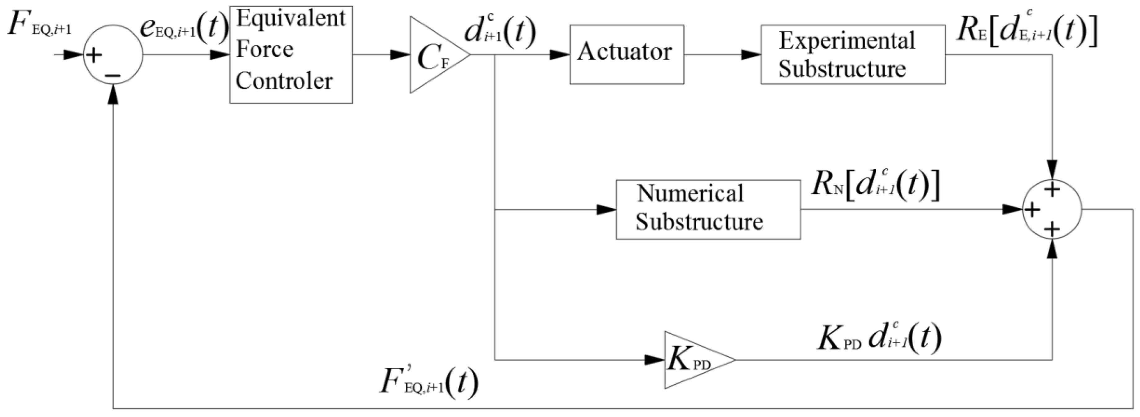
This proposed approach combines the EFC method with the proposed inflection point boundary condition technique to conduct HS tests. The EFC method is based on the feedback control method shown in Figure 4. Here, the FEQ,i+1, which is used for the equivalent force (EF) command, can be calculated by the information before the i + 1 step. Therefore, the FEQ,i+1 is available and remains unchanged at i + 1 step. The FEQ,i+1, which is used for equivalent force (EF) feedback, is obtained by the three terms: (i) the reaction of the experimental substructure , which is measured by the load cells; (ii) the reaction of the numerical substructure , which is obtained from the results of the numerical simulation; and (iii) the pseudo-dynamic force, which is linearly related to displacement by KPD. The displacement command, , is determined from the force signal using the force-displacement conversion matrix CF. The equivalent force controller is used to make certain that the EF feedback can track the EF command quickly without overshoot. This paper uses a PD controller as the equivalent force controller. The parameters of the PD controller are obtained as discussed in Reference [39].
3.3. Basic Process
Figure 5 shows the flow diagram for the proposed HS for both the virtual and the physical HS. The only difference between the virtual and the physical HS is that the physical substructure is modeled computationally. For the physical HS, the results of the physical substructure can be measured by the sensors from the model in the lab. For the virtual HS, the results of the physical substructure can be obtained from the results of an additional numerical simulation using the OpenSEES. In Figure 5, istep is the ith step of the earthquake records, and n corresponds the total number of the earthquake records. Matlab is used to integrate the EOM for calculating the responses of the structure. OpenSEES is used for simulation of the numerical substructure. The basic detailed process is as follows:
- Step 1: The initial stiffness matrix, the initial mass matrix, the initial damping matrix, other initial parameters, and the ground motion record are obtained. The ground motion record may be scaled in amplitude to accommodate the goal of different HS tests.
- Step 2: The EF command is calculated. The displacement command is then calculated using the force-displacement conversion matrix and the EF controller.
- Step 3: The pseudo-dynamic force is calculated using the pseudo-dynamic stiffness KPD, which can be determined from the initial parameters. Concurrently, the predicted axial deformation is obtained using Equation (1). Before the next step, all calculations are realized using Matlab. After this step, the calculated displacement command of the numerical substructure and the prediction axial deformation at the boundary is applied to the numerical substructure modeled by OpenSEES.
- Step 4: The calculated displacement command of the numerical substructure and the prediction axial deformation at the boundary are sent to the numerical substructure. Subsequently, the reaction force at the boundary is calculated. Similarly, the data calculated by OpenSEES are sent to the Matlab program and subsequently wait to receive the data calculated by Matlab for the next step.
- Step 5: The calculated reaction force in the vertical direction and the displacement command in the horizontal direction are sent to the actuator controllers for the physical substructure. Then, the reaction of the physical substructure is obtained by: (i) the sensors in the associated loading devices; or (ii) OpenSEES for the virtual test.
- Step 6: The EF feedback is obtained by summing up the pseudo-dynamic force, and the reaction of both the numerical substructure and the physical substructure. Then, compare the EF feedback with the EF command to obtain the error between them. If the error between the EF feedback with the EF command is less than the specified tolerance, go the next step. If not, repeat the steps from the third step to the sixth step.
- Step 7: The responses of the entire structure are obtained. Then, repeat the above-mentioned steps until the entire ground motion record has been processed.
After the details of proposed HS, a series of numerical simulation is carried out though the virtual HS in the next section. Then, experimental validation is accomplished using a six-story steel frame model. The El Centro (N-S, 1940) is taken as the ground motion record for both the virtual and the physical HS tests.
4. Numerical Simulation
4.1. Numerical Simulation Model Based on the Uniform Design
To illustrate the proposed approach, a series of steel frame structures with 3–17 stories were considered. A nonlinear Beam–column element, which has a hardening bilinear constitutive model, was chosen in OpenSEES to model the frame. The yield strength is 235 Mpa. The elastic modulus is 200,000 Mpa. The post-yield to pre-yield stiffness ratio is 0.02. The mass matrix was calculated using provision 5.1.3 of the Chinese Code for Seismic Building Design GB50011-2010. Rayleigh Damping was adopted with a damping ratio of 0.05 in the first two modes. The number of the stories in the building, the beam–column’s linear stiffness ratio (LSR), and the peak ground acceleration (PGA) of the ground motion record were taken as parameters for the numerical study. Each story height is 4 m, and the span of the steel frame structure is 6 m.
This experimental design method proposed by Wang and Fang [40] was used to increase efficiency and reduce the required number of tests by focusing on the uniformity of the test matrix. For example, assume that the m parameters are chosen in an experiment. Let the number of values of each parameter to be considered be n. The number of experiments is mn for a full factorial design. The number of samples is about m2 for an orthogonal design, which takes both the orthogonality and uniformity of the design space into consideration. However, the number of experiments is about m for the uniform design, which only highlights the uniformity of the design space.
The uniform design table, Un(qs), which is similar to the orthogonal design table, was constructed in advance, where the symbol U is the label for the uniform design, n is the number of test, s is the maximum number of parameters, and q is the number of levels for each parameter. The deviation D of the uniform design table is taken as the index to evaluate the uniformity of the table. The smaller is the value of D, the better is the uniformity of the design table. By considering the number of stories, the beam–column’s linear stiffness ratio, and the peak ground acceleration (PGA) of the ground motion record, the uniform design table U*15(157) was chosen. The symbol * means that the design table has more uniformity [40]. The deviation D of the selected uniform table is 0.1361, which meets the precision required. More detailed parameters are listed in Table 1.
4.2. Numerical Simulation Results Analysis
This section provides a comparison of the numerical simulation for each model listed in Table 1 for the traditional technique and the proposed elastic inflection point technique. The simulation result of entire structure using OpenSEES is considered to be the “exact” solution and used as a point of reference. The errors in the numerical simulation for the different boundary simulation techniques at the ith step, as compared to the reference solution, are designated as ei. Then, the cumulative error in the numerical simulation for the different boundary simulation techniques is given by
Due to space limitation, only representative results are given for three of these buildings: tests No. 2, No. 8, and No. 13.
4.2.1. Displacements Analysis
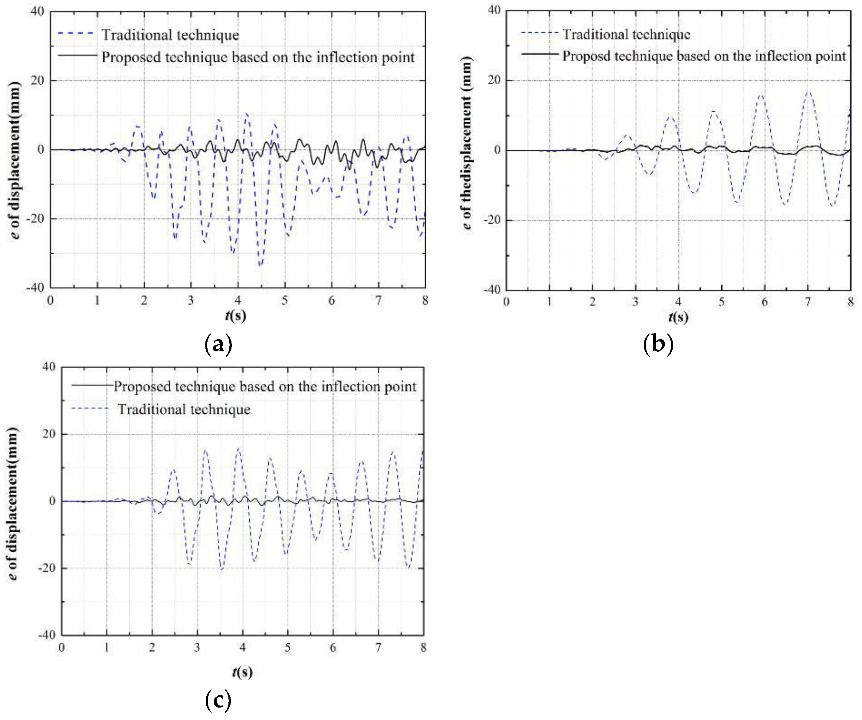
Figure 6 shows the time history of the errors ei for tests No. 2, No. 8, and No. 13 for the traditional and proposed boundary simulation techniques. In Figure 6, we can see clearly that the error in the displacement for the proposed boundary technique is smaller than the traditional technique. The simulation results for the other numerical tests shown in Table 1 followed similar trends. Additionally, the maximum displacement errors and the cumulative errors for the different boundary techniques were calculated for the 15 tests shown in Table 1. The mean of the maximum displacement error and the mean of the cumulative error over all 15 tests was calculated for both the traditional technique and the proposed technique. Both error measures were found to be an order of magnitude smaller for the proposed approach, as compared with the traditional technique. The maximum displacement error ratio between two different techniques had an average of 9.18 with a maximum of 13.00 and a minimum of 2.66. The cumulative error ratio between two different techniques had an average of 9.87 with a maximum of 18.04 and a minimum of 3.12.
4.2.2. Internal Force Analysis
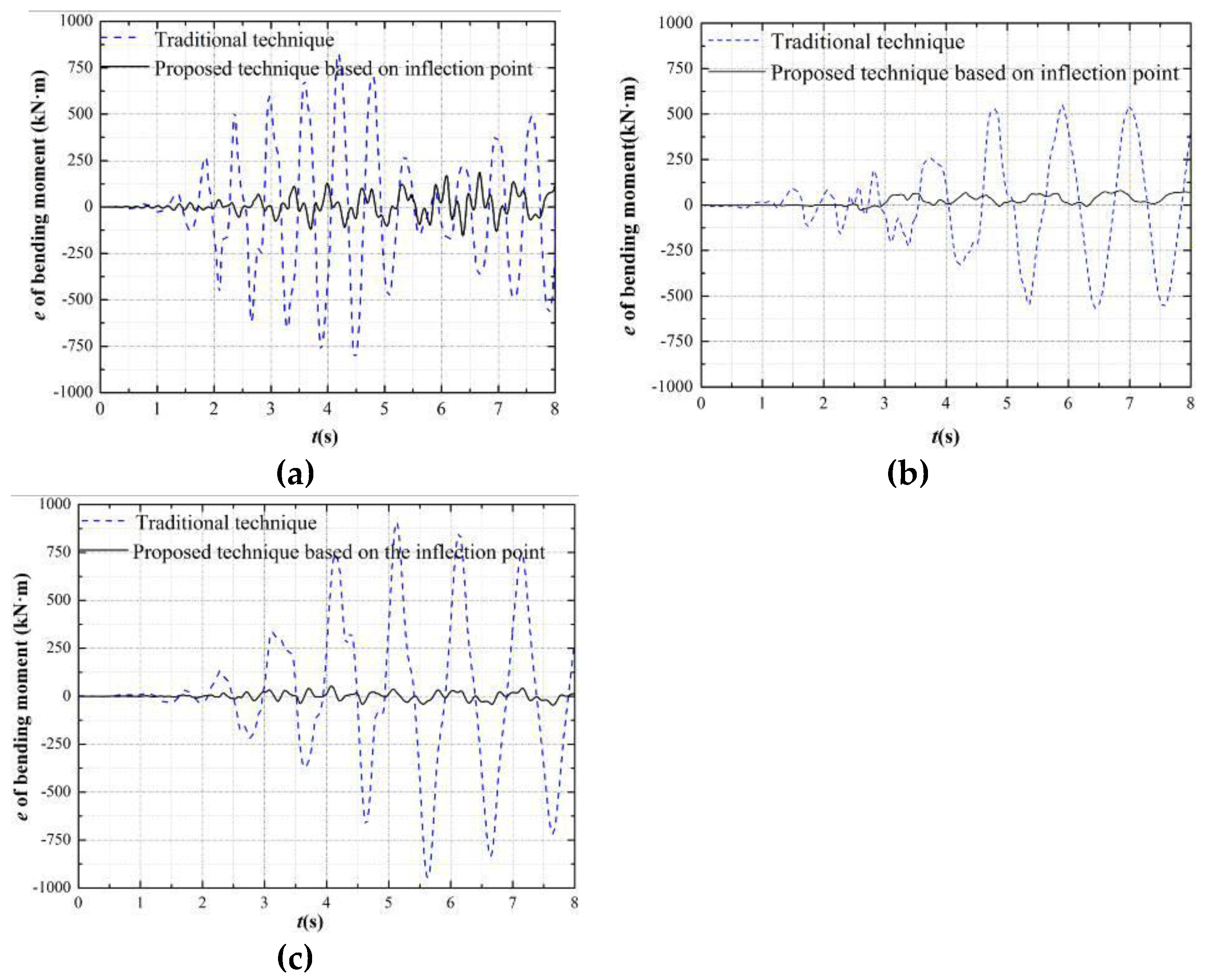
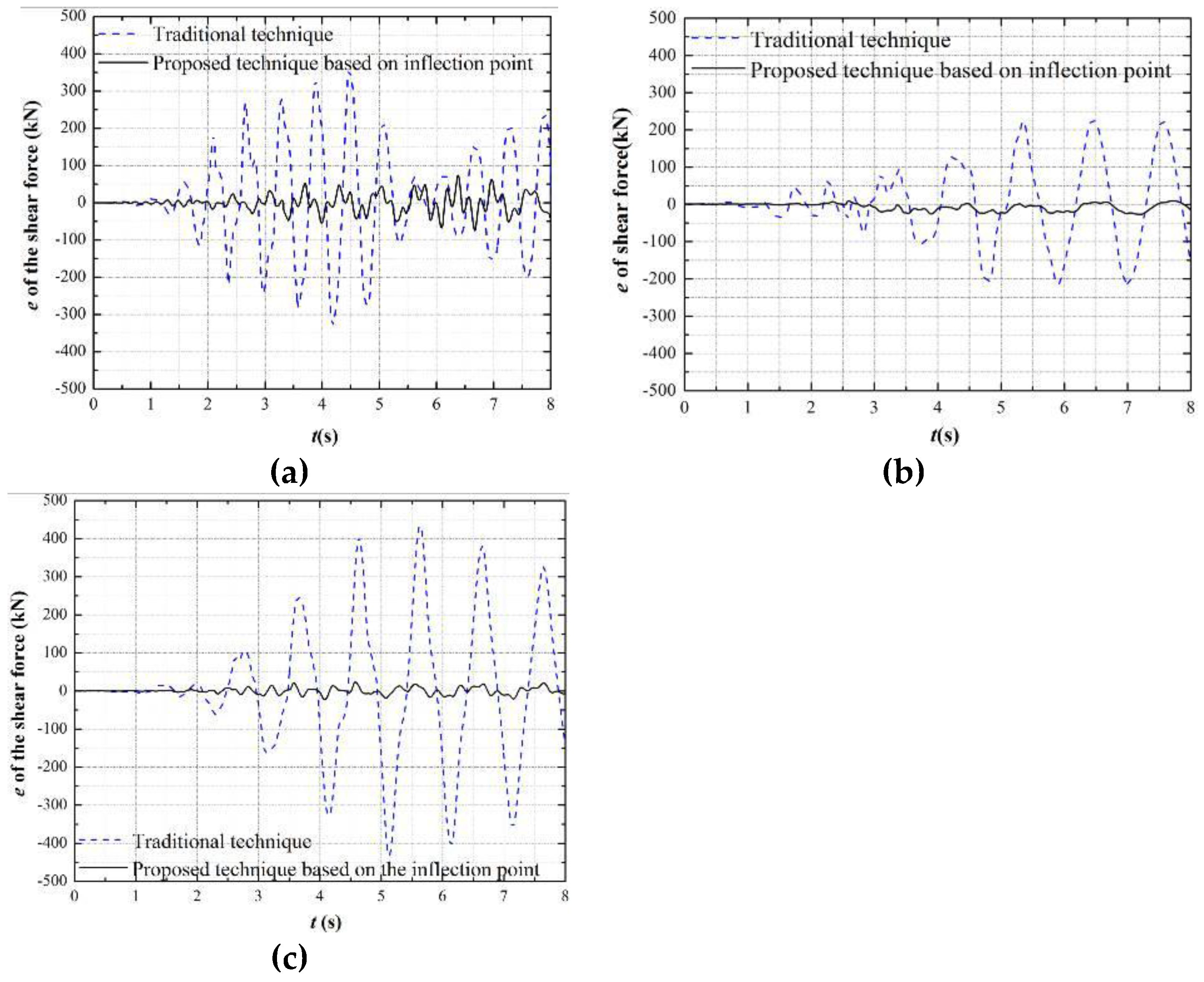
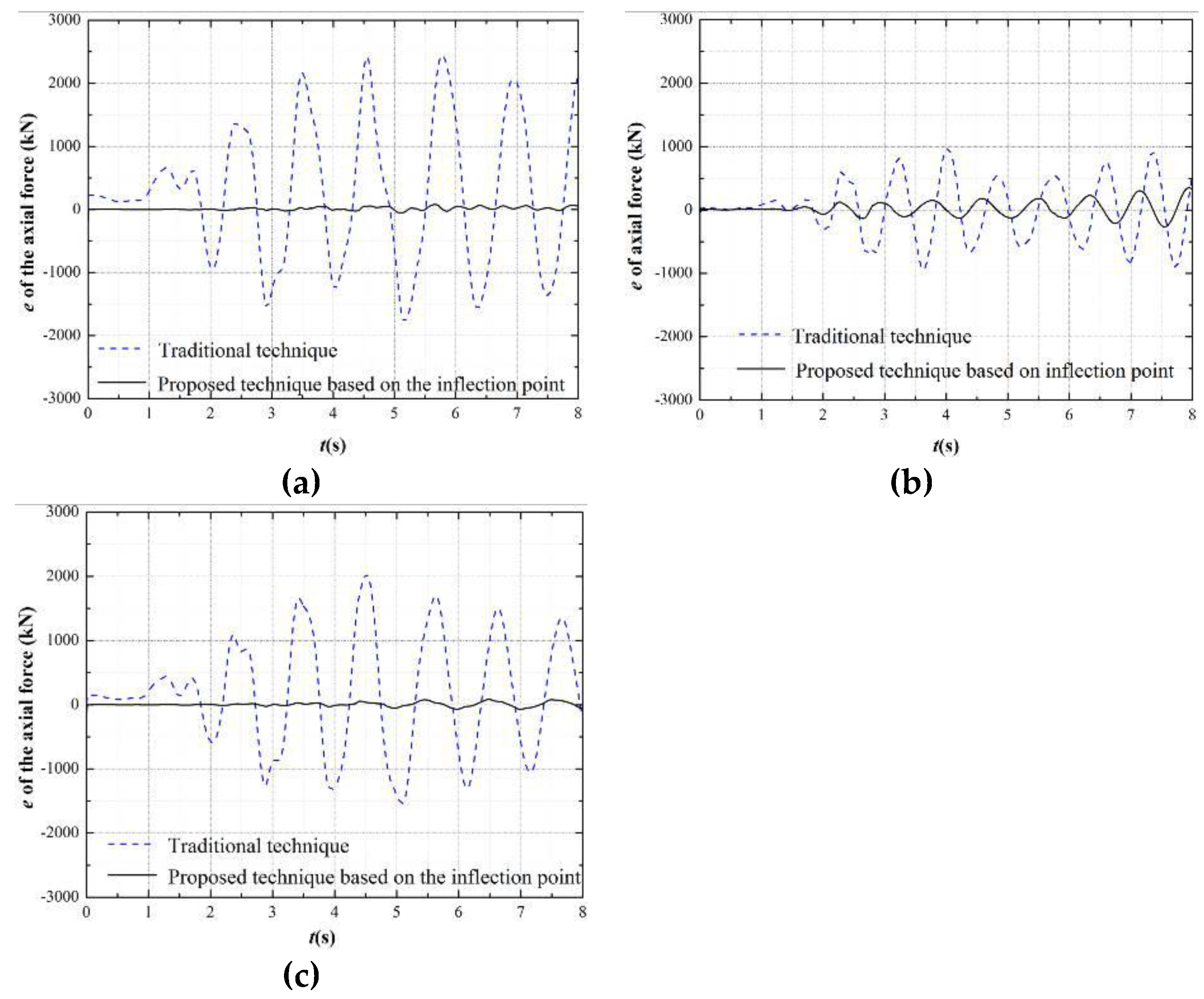
Figure 7, Figure 8 and Figure 9 show the error time history of the bending moment, shear force, and axial force, respectively, at the top of the column of the 1st story for the different boundary techniques. Here, the internal force (including bending moment, shear force, and axial force) errors have a similar tendency with the displacement errors in Section 4.2.1. The internal force errors of the proposed boundary technique based on the inflection point are the smaller than the traditional one.
The maximum internal forces (the bending moment, the shear force and the axial force) errors and the cumulative errors of different boundary techniques at the top of the first story column follow a similar tendency with the displacement. The means of maximum errors ratio and the cumulative errors ratio of the bending moment between the traditional and proposed technique are 4.86 and 9.42, respectively. Both the shear force and the axial force have a similar tendency but the means of the corresponding ratio are larger than the bending moment. The means of maximum errors ratio and the cumulative errors ratio of the shear force are 9.44 and 12.90, respectively. The means of maximum errors ratio and the cumulative errors ratio of the axial force are 17.62 and 23.65, respectively.
Therefore, these results demonstrate that the proposed technique based on the inflection point can improve substantially the test accuracy and show the better performance than the traditional method.
5. Experimental Validation
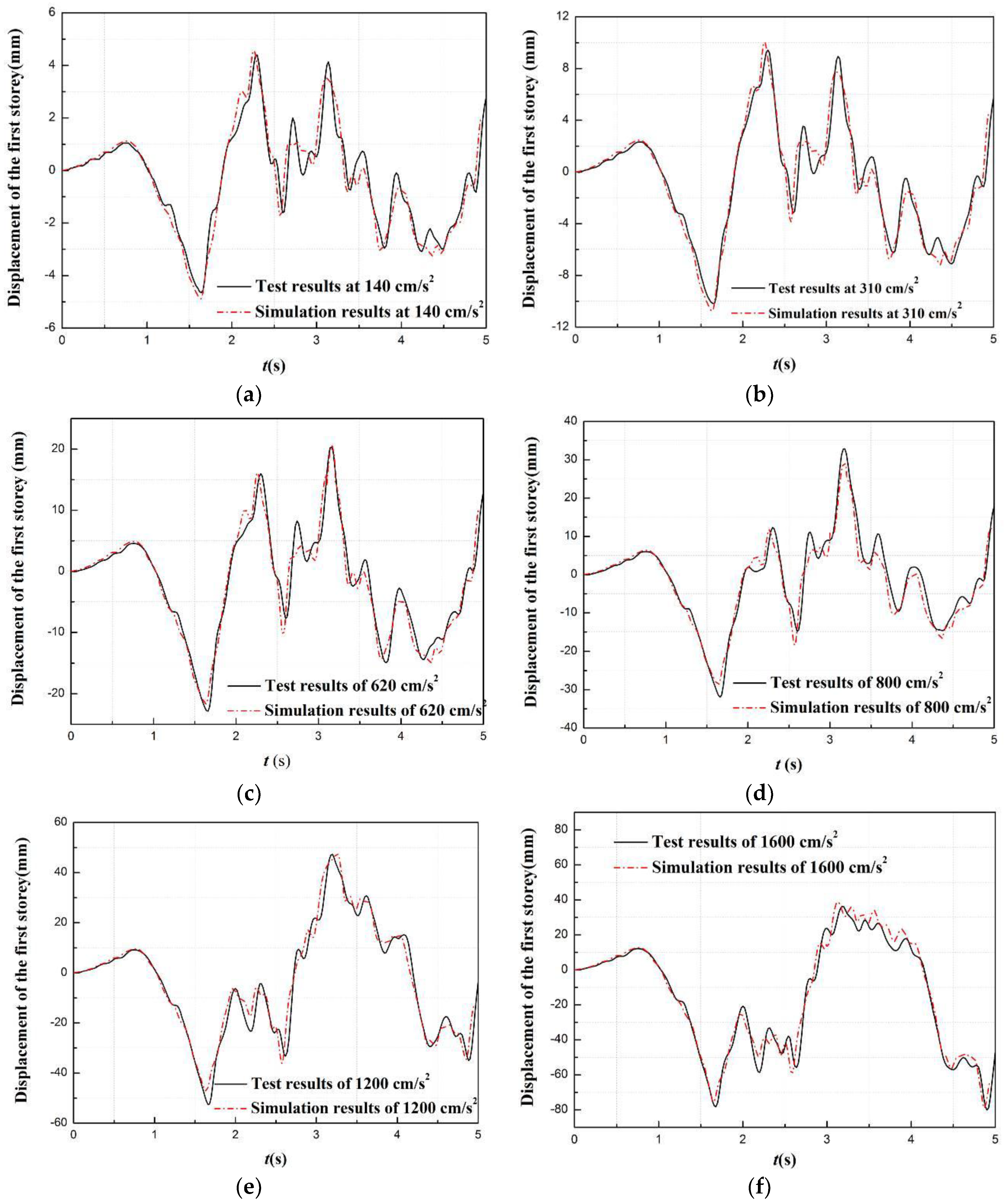
To validate the proposed boundary method, a six-story steel frame structure, in which the first story was taken as the physical substructure and the rest of the structure as the numerical substructure, was designed as the HS testing model. Ground motions with PGAs of 310, 620, 800, 1200, and 1600 cm/s2 were sequentially applied to the test structure.
5.1. Test Model
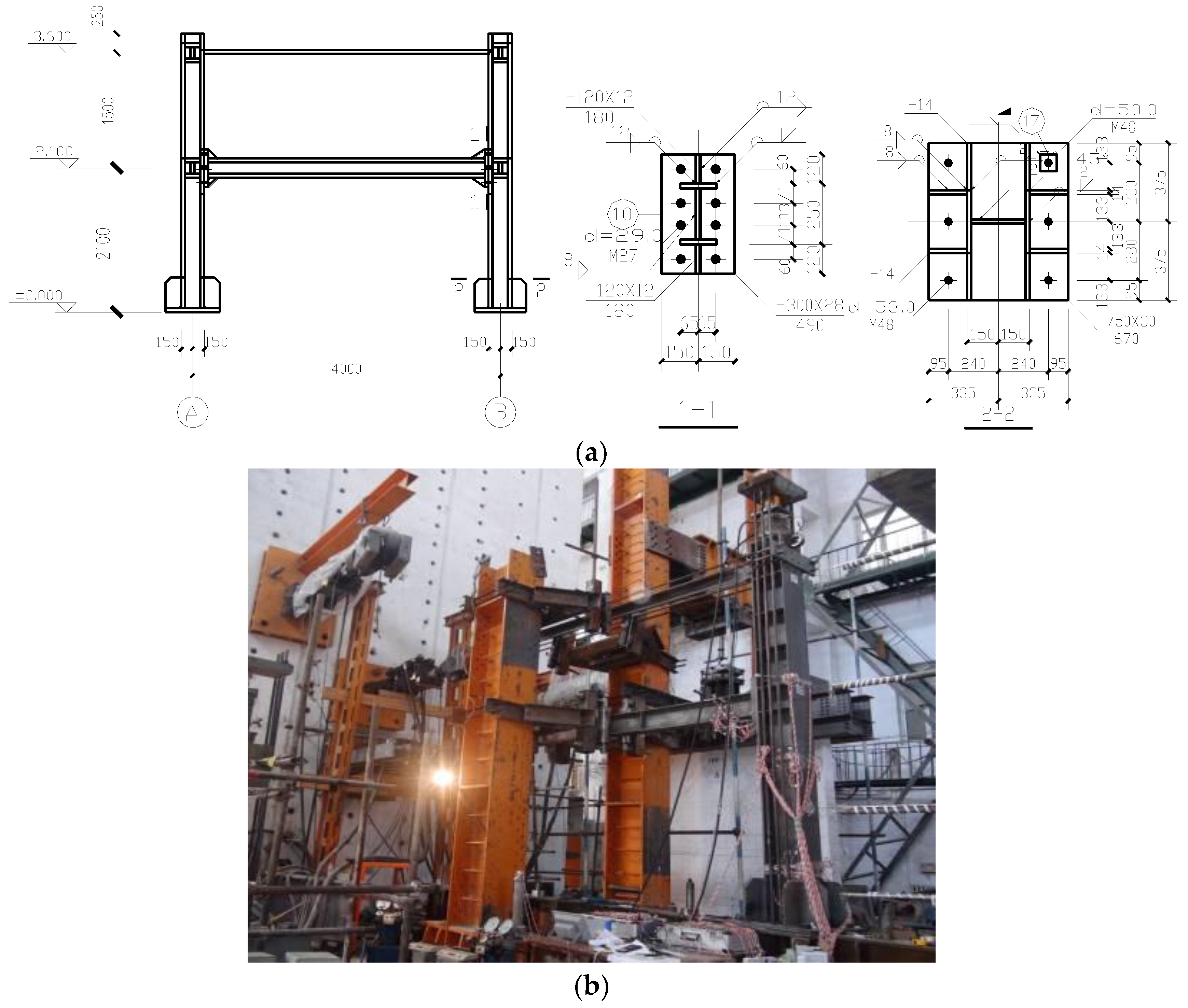
The six-story frame structure was designed based on both Chinese Code GB50017-2003 for Design of Steel Structures and Chinese Code for Seismic Building Design GB50011-2010. The height of the first story is 4200 mm and others are 4000 mm. The span of the bay for the test model is 8000 mm. The sections of the columns are HW600 × 600 × 20 × 30, and the section of the beams are HW500 × 300 × 14 × 22 (with units of mm). Q235 steel is used. Because of laboratory limitations, a 1/2-scale test model was manufactured in the Seismic Experimental Center of Civil Engineering at the Harbin Institute of Technology.
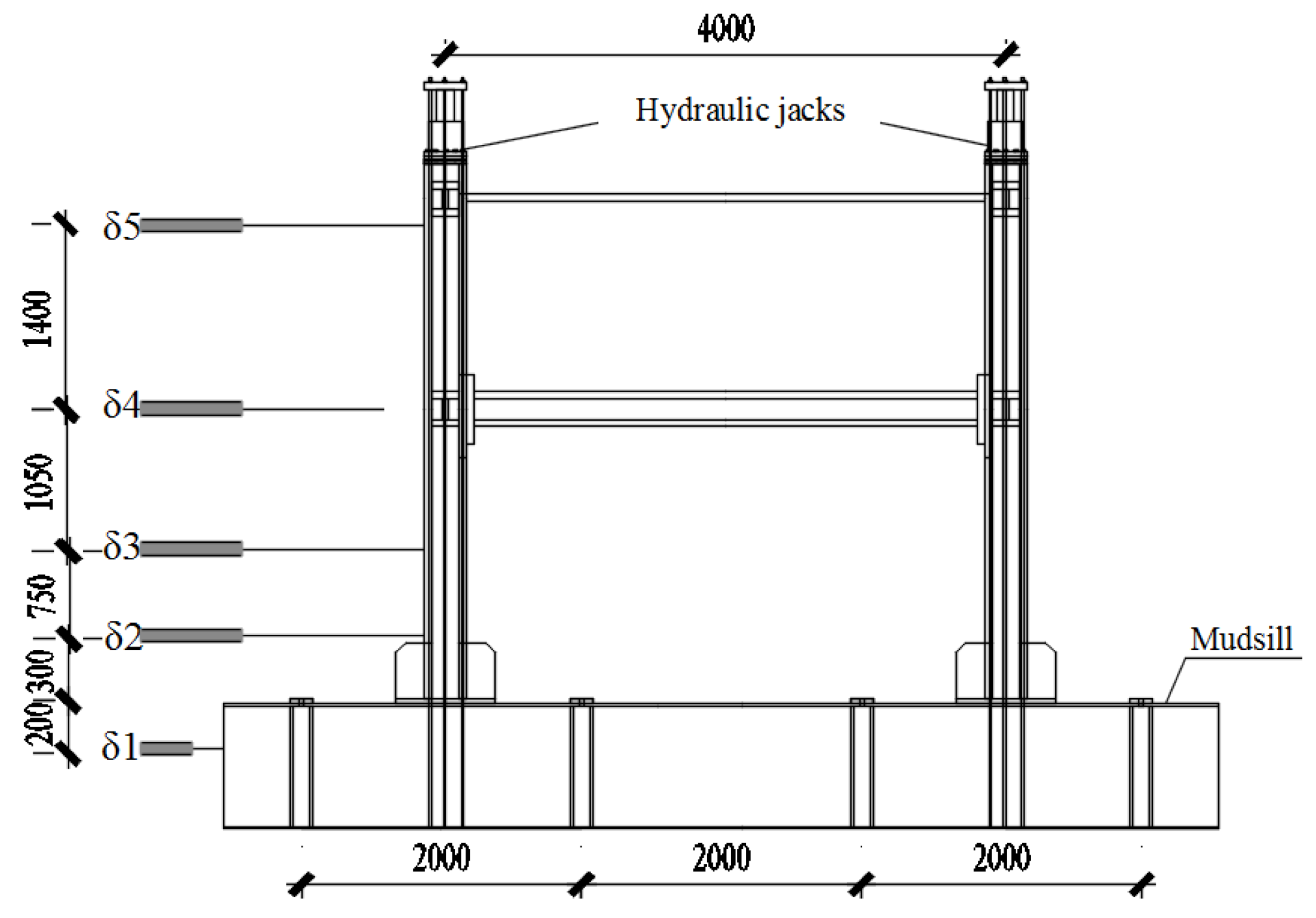
The first story, along with the columns of the second story up to the inflection point, was taken as the physical substructure for the proposed boundary technique, as illustrated in Figure 10. A transfer-structure, which is hinge connected with the inflection point of both columns by the high-strength bolts M10.9, was designed to realize the synchronous horizontal displacement by using the two-equilateral angle steel 100 × 10 (mm). The physical experiment is shown in Figure 11, and Table 2 provides the test results for the performance of the steel material. The mass of the first–fifth stories m1–5 = 88,000 kg, and the mass of the topper story m6 = 84,000 kg. The record of the ground motion is the El Centro. Rayleigh Damping is chosen, with parameters a is 0.115 and b is 0.0024, corresponding to 5% damping in the first two modes.
5.2. Displacement–Force Mixed Control Technique
The traditional HS test, which usually focuses on the compatibility and equilibrium only in the horizontal direction, is conducted using the displacement control. The calculated displacements obtained by solving the EOM were applied to the physical substructure test model. Then, the reaction forces corresponding to the command displacements were measured and fed back to the EOM for the calculation of the next displacement increment. The stiffness of the columns in the vertical (axial) direction is typically high, consequently making displacement control challenging to implement, primarily because the resolution of the displacement transducer used for feedback is inadequate. Therefore, force control was used to realize the axial loading in the proposed approach. To address the problem of measuring the axial displacement of the column, the technique proposed in Section 3.2 for predicting the axial displacement was employed.
To realize the displacement–force mixed control, the arrangement of the vertical and horizontal loading devices was designed as shown in Figure 12. Two hydraulic jacks were chosen as the vertical loading devices while two hydraulic servo actuators as the horizontal loading devices.
5.2.1. Vertical Loading Devices
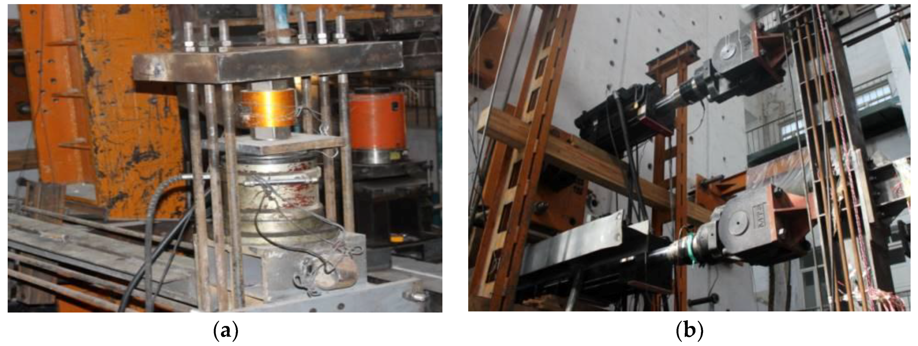
Figure 13a shows the vertical loading devices which are two hydraulic jacks. The hydraulic jacks were arranged at the boundary of the physical substructure model where the self-balancing device (Figure 13a) was designed to realize the axial load at the boundary. The self-balancing device includes the 20 mm-thick steel plate which is placed on the top of the hydraulic jack and four 25 mm-diameter steel bars which connects the 20 mm-thick steel plate and the mudsill of the physical substructure model. The loading capacity of the hydraulic jacks is 1000 kN. The loading errors are 1% of the loading capacity.
5.2.2. Horizontal Loading devices
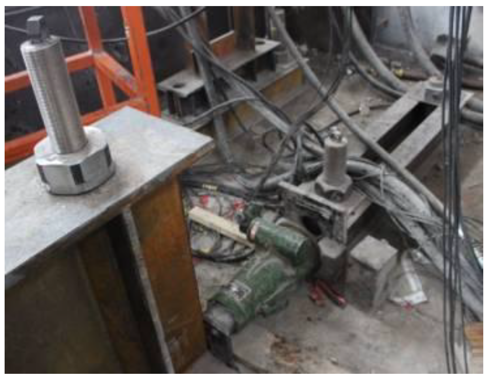
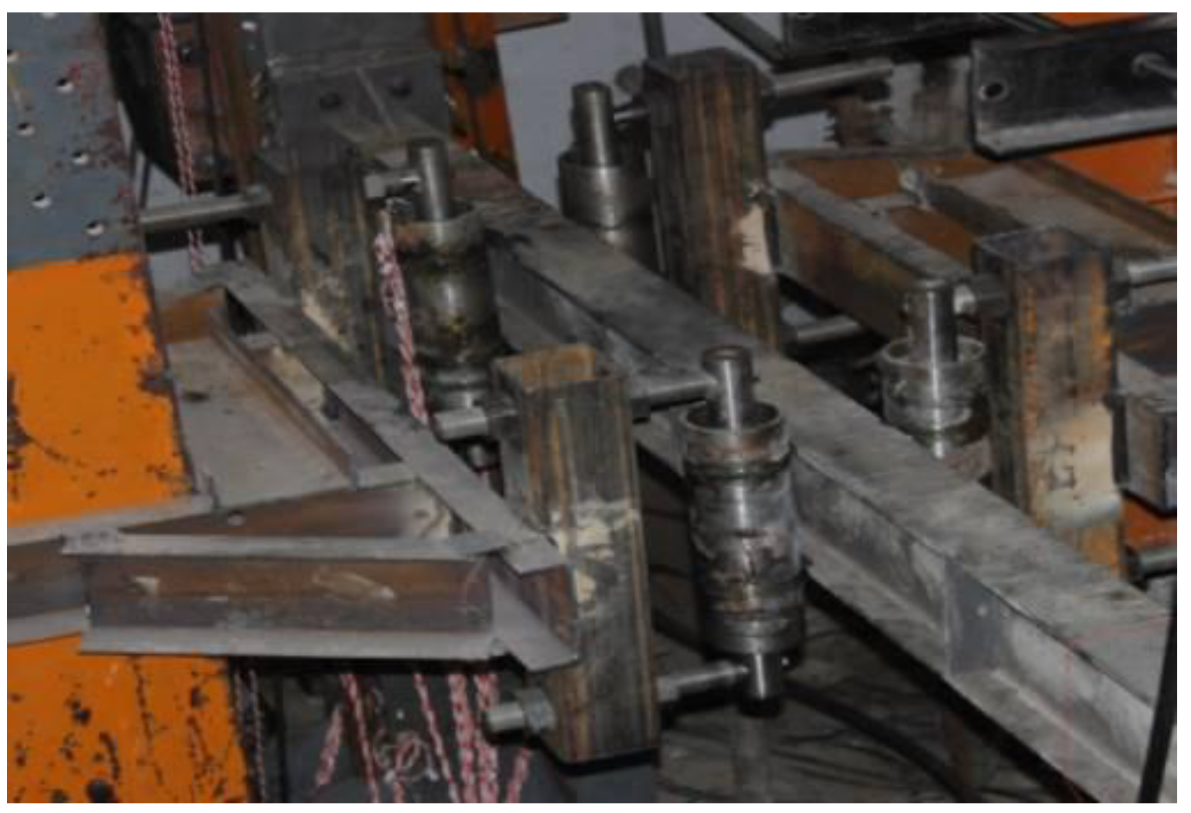
Figure 13b shows the horizontal loading devices which are two hydraulic servo actuators. One end of the hydraulic servo actuators is fixed into the actuator wall by four 100 mm-diameter bolt bars. The other end of the hydraulic servo actuators connects with the physical substructure model, in which one is located at the beam–column joint of the first story while the other at the boundary of the physical substructure model. The force capacity of two hydraulic servo actuators is ±1000 kN, and the displacement capacity is ±100 mm. The errors of both force and displacement are the 0.1% of the corresponding capacity. To avoid the horizontal slip of the physical substructure model, two measures were designed: one is that the mudsill of the physical substructure model is fixed on the floor of the lab by using 100 mm-diameter bolts spaced on 1 m centers; and the other is that two hydraulic jacks are used on both sides of the mudsill to apply the equal and opposite forces (Figure 14). In addition, four steel rollers were used on the side of both the first beam and the truss at the boundary, to avoid the out-of-plane deformation of the steel frame (Figure 15).
5.3. Arrangement of the Measurement Devices
5.3.1. Arrangement of Displacement Measuring Points
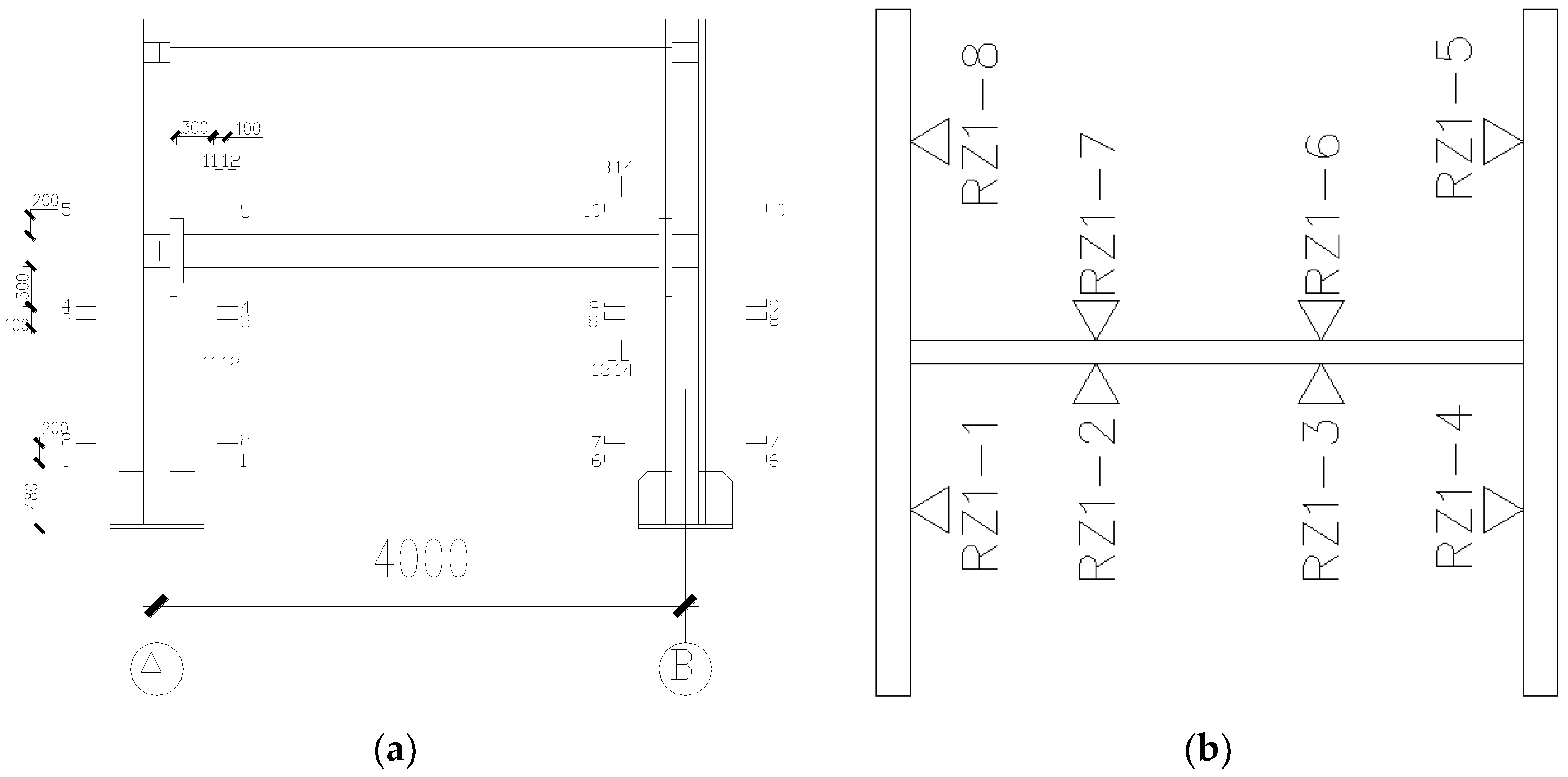
Five linear variable differential transformers (LVDTs) were employed to measure the physical displacements of the substructure model. One of the LVDTs is placed at the mudsill to measure the slip of the physical substructure model. Two of the LVDTs, which are 300 and 1050 mm above the top of the mudsill, are placed on the column. One of the LVDTs is placed at the beam–column joint of the first story, and one of the LVDTs is placed at the boundary of the physical substructure model. The stroke of all the used LVDTs is ±150 mm. The errors of the LVDTs are 0.1% of the corresponding capacity.
5.3.2. Arrangement of Strain Gauge
Figure 16a shows the arrangement of strain gauges. Each column has five sections which are chosen to paste the strain gauges. Both the top and bottom of the first column has two sections, respectively. The bottom of the second column has one section. Each end of the first beam has two sections which are chosen to paste the strain gauges. Each section has eight strain gauges to calculate the bending moment and axial force of the section (see Figure 16b).
5.4. Test Results and Analysis
Figure 17 shows the comparison curves of time history between the test results and the simulation results at the first story for different levels of PGA. The results in Figure 17 were obtained by simulating the entire structure in OpenSEES, based on the parameters in Section 5.1. The HS test results are close to the simulation results at the different PGA levels.
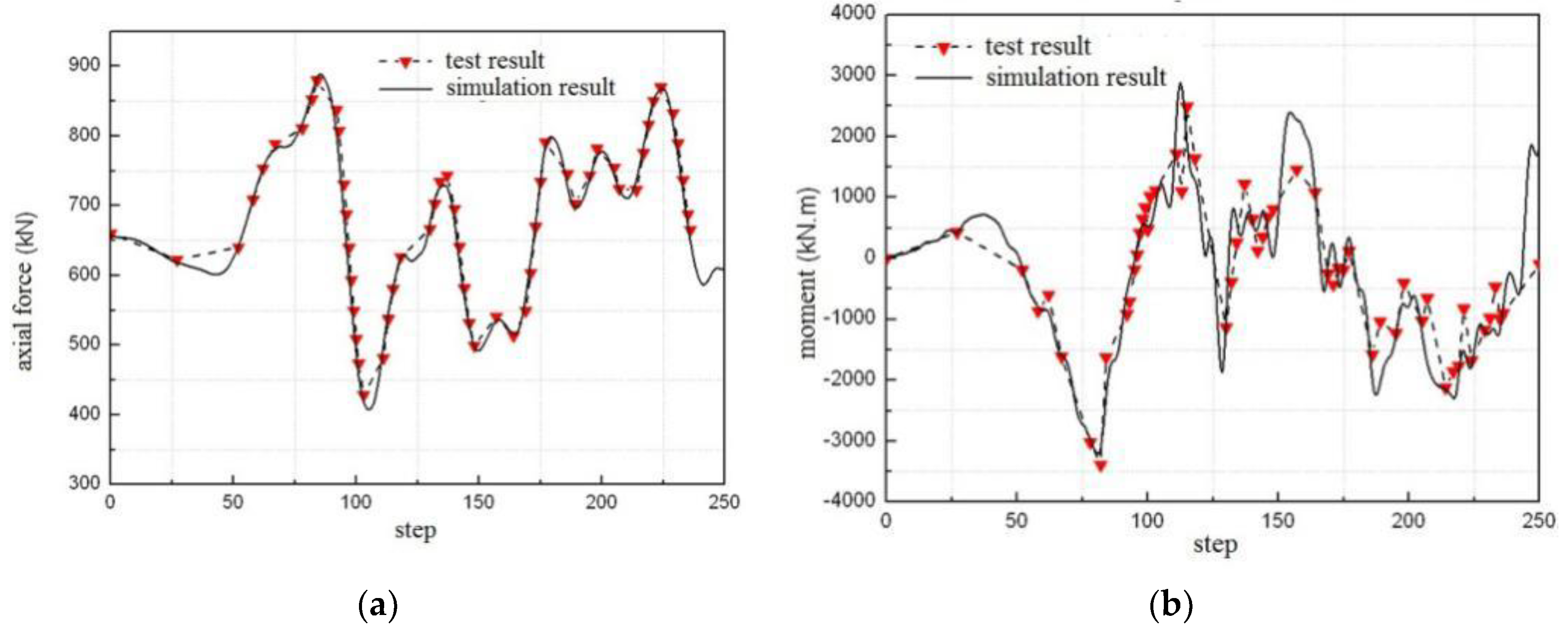
Figure 18 and Figure 19 show the comparison curves of the internal force time history between the test results and the simulation results with the 310 and 620 cm/s2, respectively. Note that, for PGA levels above 620 cm/s2, the response of the HS test model is significantly nonlinear, resulting in failure of most of the strain gauges; as a result, the internal forces calculated using the stain response are not available above a PGA of 620 cm/s2.
The shear force in Figure 18 and Figure 19 can be obtained conveniently from the force sensor of the horizontal hydraulic actuators. The bending moment and axial force can be calculated from the stain gauges of the calculated section by the following equation:
where ξi is measured by the stain gauge at the section, ξ1 and ξ8 are two compressed strain gauges at the flange of the section, ξ4 and ξ5 are two tensile strain gauges at the flange of the section, E is the elasticity modulus, I is the sectional inertia moment, A is the sectional area, y is the distance between the point for the stain gauge to the center of the section, N is the axial force on the section, and M is the bending moment. Because the measure of the stain gauge is only recorded at the step when the vertical force changes, Figure 18 and Figure 19 give the calculated values of the bending moment and the axial force at the recorded step.
Figure 18 and Figure 19 also show that the test results of internal forces are close to the simulation one. Table 3 gives the relative errors at the peak of the internal force. In Table 3, the maximum relative error is less than 10%, showing good performance of the proposed boundary technique based on the inflection point.
6. Conclusions
This paper proposes a new boundary technique based on the inflection point, where the bending moment is zero, to conveniently realize the equilibrium and compatibility at the boundary. The axial displacement prediction technique is used to meet the equilibrium and compatibility of the axial direction at the boundary. To realize the process of the HS based on the proposed boundary technique, the HS component interaction is used to build a bridge between the Matlab and the OpenSEES, and the equivalent force control method is employed for solution of the EOM. Comparison of the results of the numerical simulation and the physical test show that the proposed method has the better performance than the traditional boundary technique.
Fifteen numerical examples are presented to verify the accuracy and feasibility of the proposed boundary technique. The numerical simulation results show that the proposed technique based on the inflection point can improve tremendously the test accuracy over the traditional technique.
The systematic laboratory hybrid simulation tests of the six-story steel frame structure model were designed to verify the accuracy and feasibility of the proposed boundary technique. The displacement–force mixed control technique is proposed to realize the real hybrid simulating test based on the proposed boundary technique. The tests results show reliable and accurate performance of proposed boundary technique.
Author Contributions
All authors made substantial contributions to this study. Z.C. provided the concept and design of the study. X.Y. and X.Z. performed the experiment and collected the data. H.W. and B.F.S. wrote and revised the manuscript. Z.C., X.Y. and X.Z. analyzed the experimental data.
Funding
The research is financially supported by the Natural Science Foundation of China (51678199, 51578151, and 51161120360).
Acknowledgments
The authors gratefully acknowledge the financial support provided by the China Scholarship Council (CSC) at UIUC in 2016 (201606125079).
Conflicts of Interest
The authors declare no conflict of interest.
References
- Hakuno, M.; Shidowara, M.; Haa, T. Dynamic destructive test of a cantilevers beam, Controlled by an analog-computer. Trans. Jpn. Soc. Civ. Eng. 1969, 171, 1–9. [Google Scholar] [CrossRef]
- Takanashi, K.; Nakashima, M. Japanese activities on online testing. J. Eng. Mech. 1987, 113, 1014–1032. [Google Scholar] [CrossRef]
- Mahin, S.A.; Shing, P.B.; Thewalt, C.R.; Hanson, R.D. Pseudodynamic test method current status and future directions. J. Struct. Eng. 1989, 115, 2113–2128. [Google Scholar] [CrossRef]
- Shing, P.B.; Nakashima, M.; Bursi, O.S. Application of psuedodynamic test method to structural research. Earthq. Spectr. 1996, 12, 29–56. [Google Scholar] [CrossRef]
- Saouma, V.; Sivaselvan, M. Hybrid Simulation: Theory, Implementation and Applications; Taylor & Francis: London, UK, 2008; ISBN 978-0-415-46568-7. [Google Scholar]
- Bursi, O.S.; Wagg, D. Modern Testing Techniques for Structural Systems: Dynamics and Control; Springer: New York, NY, USA, 2008; ISBN 978-3-211-09445-7. [Google Scholar]
- Wu, B.; Wang, Q.; Shing, P.B.; Ou, J. Equivalent force control method for generalized real-time substructure testing. Earthq. Eng. Struct. Dyn. 2007, 36, 1127–1149. [Google Scholar] [CrossRef]
- Wallace, M.I.; Sieber, J.; Neild, S.A.; Wagg, D.J.; Krauskopf, B. Stability analysis of real-time dynamic substructuring using delay differential equation models. Earthq. Eng. Struct. Dyn. 2005, 34, 1817–1832. [Google Scholar] [CrossRef] [Green Version]
- Ahmadizadeh, M.; Mosqueda, G.; Reinhorn, A.M. Compensation of actuator delay and dynamics for real-time hybrid structural simulation. Earthq. Eng. Struct. Dyn. 2008, 37, 21–42. [Google Scholar] [CrossRef]
- Chen, C.; Ricles, J.M.; Marullo, T.; Mercan, O. Real-time hybrid testing using the unconditionally stable explicit CR integration algorithm. Earthq. Eng. Struct. Dyn. 2009, 38, 23–44. [Google Scholar] [CrossRef]
- Amin, M.; Shirley, D.; Siamak, R.; Arun, P. Predictive stability indicator: A novel approach to configuring a real-time hybrid simulation. Earthq. Eng. Struct. Dyn. 2017, 46, 95–116. [Google Scholar]
- Ou, G.; Ozdagli, A.I.; Dyke, S.J.; Wu, B. Robust integrated actuator control experimental verification and real-time hybrid simulation implementation. Earthq. Eng. Struct. Dyn. 2015, 44, 441–460. [Google Scholar] [CrossRef]
- Phillips, B.M.; Takada, S.; Spencer, B.F.; Fujino, Y. Feedforward actuator controller development using the backwarddifference method for real-time hybrid simulation. Smart Struct. Syst. 2014, 14, 1081–1103. [Google Scholar] [CrossRef]
- Friedman, A.; Dyke, S.J.; Phillips, B.; Ahn, R.; Dong, B.; Chae, Y.; Castaneda, N.; Jiang, Z.; Zhang, J.; Cha, Y.; et al. Large-scale real-time hybrid simulation for evaluation of advanced damping system performance. J. Struct. Eng. 2015, 141, 04014150. [Google Scholar] [CrossRef]
- Gao, X.; Castaneda, N.; Dyke, S.J. Real-time hybrid simulation: From dynamic system, motion control to experimental error. Earthq. Eng. Struct. Dyn. 2013, 42, 815–832. [Google Scholar] [CrossRef]
- Takahashi, Y.; Fenves, G. Software framework for distributed experimental-computational simulation of structural systems. Earthq. Eng. Struct. Dyn. 2006, 35, 267–291. [Google Scholar] [CrossRef]
- Kwon, O.S.; Elnashai, A.S.; Spencer, B.F. UI-SIMCOR: A global platform for hybrid distributed simulation. In Hybrid Simulation: Theory, Implementation and Applications; CRC Press: Boca Raton, FL, USA, 2008; pp. 157–167. [Google Scholar]
- Pan, P.; Tomofuji, H.; Wang, T.; Nakashima, M.; Ohsaki, M.; Mosalam, K.M. Development of peer-to-peer (P2P) internet online hybrid test system. Earthq. Eng. Struct. Dyn. 2006, 35, 867–890. [Google Scholar] [CrossRef]
- Guo, Y.R.; Zhu, X.J.; Wang, Z.M.; Zhang, Z.X. A NetSLab Based Hybrid Testing Program for Composite Frame Structures with Buckling Restrained Braces. Adv. Mater. Res. 2013, 639–640, 1142–1147. [Google Scholar] [CrossRef]
- Buckle, I.; Reitherman, R. The consortium for the George E. Brown J. network for earthquake engineering simulation. In Proceedings of the 13th World Conference on Earthquake Engineering, Vancouver, BC, Canada, 1–6 August 2004; p. 4016. [Google Scholar]
- Stojadinovic, B.; Mosqueda, G.; Mahin, S.A. Event-driven control system for geographically distributed hybrid simulation. J. Struct. Eng. 2006, 132, 68–77. [Google Scholar] [CrossRef]
- Kim, J.K. KOCED collaboratory program. In Proceedings of the Annual Meeting: Networking of Young Earthquake Engineering Researchers and Professionals (ANCER), Hawaii, HI, USA, 2004. [Google Scholar]
- Ohtani, K.; Ogawa, N.; Katayama, T.; Shibata, H. Project ‘E-Defense’ (3-D Full-Scale Earthqyake Testing Facility). In Proceedings of the Joint NCREE/JRC Workshop on International Collaboration on Earthquake Disaster Mitigation Research, Taipei, Taiwan, 17–18 November 2003. [Google Scholar]
- Elnashai, A.S.; Spencer, B.F.; Kuchma, D.A.; Yang, G.; Carrion, J.E.; Gan, Q.; Kim, S.J. The multi-Axial full-scale sub-structured testing and simulation (MUST-SIM) facility at the University of Illinois at Urbana-Champaign. In Advances in Earthquake Engineering for Urban Risk Reduct; Kluwer Academic Publishers: Alphen aan den Rijn, The Netherlands, 2006; pp. 245–260. [Google Scholar]
- Fermandois-Cornejo, G.; Spencer, B.F. Framework development for multi-axial real-time hybrid simulation testing. In Proceedings of the 16th World Conference on Earthquake Engineering, Santiago, Santiago Metropolitan Region, Chile, 9–13 January 2017; p. 2770. [Google Scholar]
- Hashemi, M.J.; Tsang, H.-H.; Al-Ogaidi, Y.; Wilson, J.L.; Al-Mahaidi, R. Collapse Assessment of Reinforced Concrete Building Columns through Multi-Axis Hybrid Simulation. ACI Struct. J. 2017, 114, 437–449. [Google Scholar] [CrossRef]
- Gao, X.; Castaneda, N.; Dyke, S. Experimental Validation of a Generalized Procedure for MDOF Real-Time Hybrid Simulation. J. Eng. Mech. 2014, 140, 04013006. [Google Scholar] [CrossRef]
- Murray, J.A.; Sasani, M. Collapse Resistance of a Seven-Story Structure with Multiple Shear-Axial Column Failures Using Hybrid Simulation. J. Struct. Eng. 2016, 143, 04017012. [Google Scholar] [CrossRef]
- Kammula, V.; Erochko, J.; Kwon, O.; Christopoulos, C. Application of hybrid-simulation to fragility assessment of the telescoping self-centering energy dissipative bracing system. Earthq. Eng. Struct. Dyn. 2014, 43, 811–830. [Google Scholar] [CrossRef]
- Chae, Y.; Ricles, J.M.; Sause, R. Large-scale real-time hybrid simulation of a three-story steel frame building with magneto-rheological dampers. Earthq. Eng. Struct. Dyn. 2014, 43, 1915–1933. [Google Scholar] [CrossRef]
- Dong, B.; Sause, R.; Ricles, J.M. Accurate real-time hybrid earthquake simulations on large-scale MDOF steel structure with nonlinear viscous dampers. Earthq. Eng. Struct. Dyn. 2015, 44, 2035–2055. [Google Scholar] [CrossRef]
- Abbiati, G.; Bursi, O.S.; Caperan, P.; Sarno, L.D.; Molina, F.J.; Paolacci, F.; Pegon, P. Hybrid simulation of a multi-span RC viaduct with plain bars and sliding bearings. Earthq. Eng. Struct. Dyn. 2015, 44, 2221–2240. [Google Scholar] [CrossRef]
- Murray, J.A.; Sasani, M. Near-collapse response of existing RC building under severe pulse-type ground motion using hybrid simulation. Earthq. Eng. Struct. Dyn. 2016, 45, 1109–1127. [Google Scholar] [CrossRef]
- Shao, X.; Pang, W.; Griffith, C.; Ziaei, E.; van de Lindt, J. Development of a hybrid simulation controller for full-scale experimental investigation of seismic retrofits for soft-story woodframe buildings. Earthq. Eng. Struct. Dyn. 2016, 45, 1233–1249. [Google Scholar] [CrossRef]
- Kolay, C.; Ricles, J.M.; Marullo, T.M.; Mahvashmohammadi, A.; Sause, R. Implementation and application of the unconditionally stable explicit parametrically dissipative KR-alpha method for real-time hybrid simulation. Earthq. Eng. Struct. Dyn. 2015, 44, 735–755. [Google Scholar] [CrossRef]
- Hashemi, M.J.; Mosqueda, G. Innovative substructuring technique for hybrid simulation of multistory buildings through collapse. Earthq. Eng. Struct. Dyn. 2014, 43, 2059–2074. [Google Scholar] [CrossRef]
- Wang, T.; Mosqueda, G.; Jacobsen, A. Performance evaluation of a distributed hybrid test framework to reproduce the collapse behavior of a structure. Earthq. Eng. Struct. Dyn. 2012, 41, 295–313. [Google Scholar] [CrossRef]
- Mahmoud, H.N.; Elnashai, A.S.; Spencer, B.F.; Kwon, O.S.; Bennier, D.J. Hybrid simulation for earthquake response of semirigid partial-strength steel frames. J. Struct. Eng. 2013, 139, 1134–1148. [Google Scholar] [CrossRef]
- Chen, Z.X.; Xu, G.Sh.; Wu, B.; Sun, Y.; Wang, H.; Wang, F. Equivalent force control method for substructure pseudo-dynamic test of a full-scale masonry structure. Earthq. Eng. Struct. Dyn. 2014, 43, 969–983. [Google Scholar] [CrossRef]
- Fang, K.T.; Ma, C.X. The Uniform Design Method; Science Press: Beijing, China, 2001; ISBN 7-03-009189-2. [Google Scholar]
Figure 1.
Schematic diagram of the different boundary techniques: (a) Full model; (b) traditional technique; and (c) proposed technique. di denotes the displacements of each level on the full models. i ∈ [1, 5]. db denotes the displacements at the inflection point. δ1 and δ2 denote the axial deformation on interfaces. NG denotes the constant representative value of gravity load calculated by the numerical substructure. Nb1 and Nb2 denote the axial forces resulted from the overturning moments on physical substructure transmitted from numerical substructure on each interface.

Figure 2.
Calculation diagram for the upper story axial force of the physical substructure.

Figure 3.
Sketch of the HS component interaction.

Figure 4.
The block diagram of EFC method [39].
Figure 4.
The block diagram of EFC method [39].

Figure 5.
Flow diagram of substructure boundary simulation for the HS testing method.
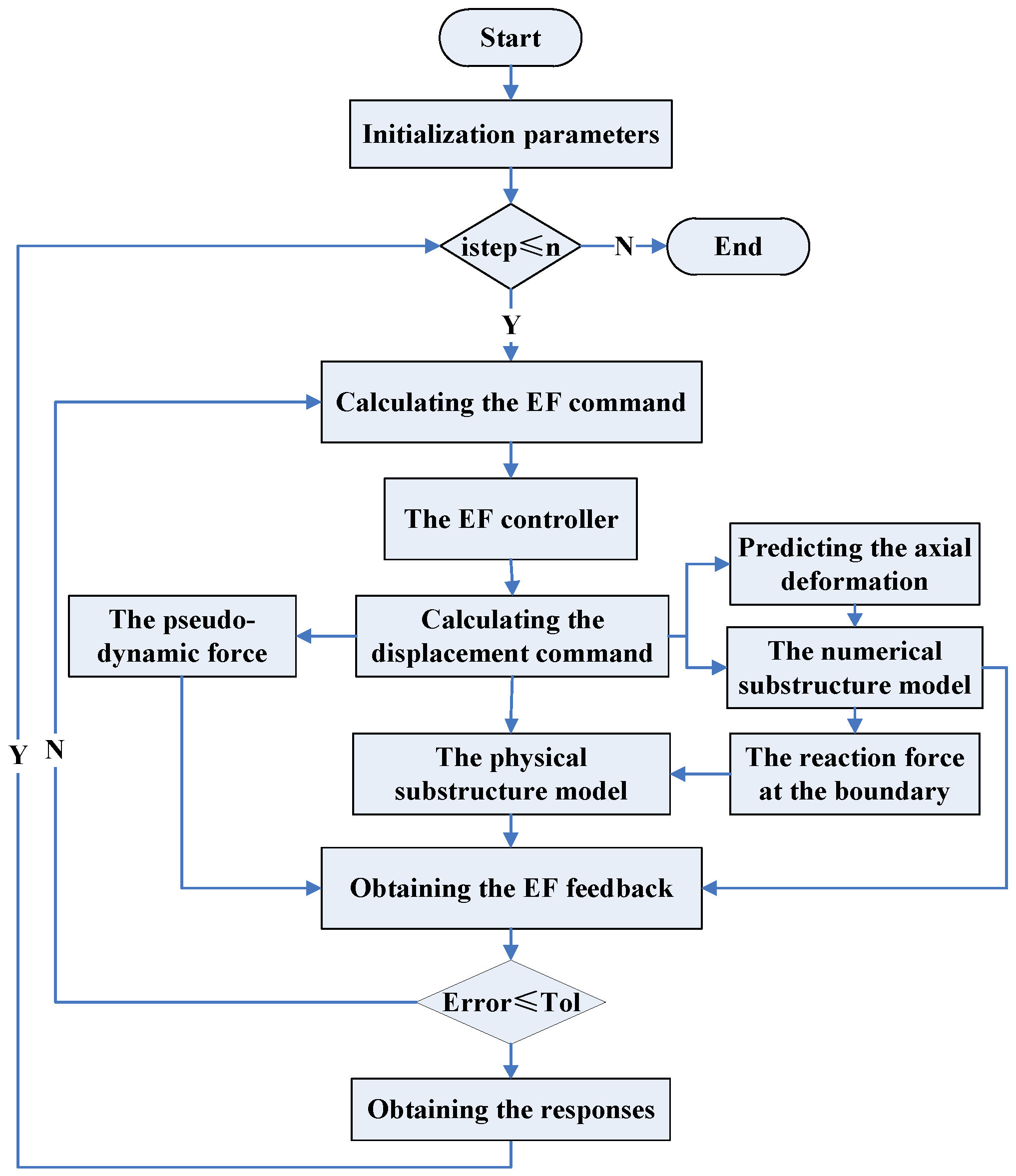
Figure 6.
The time history of the displacement errors for the different boundary techniques at the first story: (a) Test 2; (b) Test 8; and (c) Test 13.
Figure 6.
The time history of the displacement errors for the different boundary techniques at the first story: (a) Test 2; (b) Test 8; and (c) Test 13.

Figure 7.
Time history of bending moment errors for different boundary technique at the top of the column of the first story: (a) Test 2; (b) Test 8; and (c) Test 13.
Figure 7.
Time history of bending moment errors for different boundary technique at the top of the column of the first story: (a) Test 2; (b) Test 8; and (c) Test 13.

Figure 8.
Time history of shear force errors for different boundary technique at the top of the column of the first story: (a) Test 2; (b) Test 8; and (c) Test 13.
Figure 8.
Time history of shear force errors for different boundary technique at the top of the column of the first story: (a) Test 2; (b) Test 8; and (c) Test 13.

Figure 9.
Time history of axial force errors for different boundary technique at the top of the column of the first story: (a) Test 2; (b) Test 8; and (c) Test 13.
Figure 9.
Time history of axial force errors for different boundary technique at the top of the column of the first story: (a) Test 2; (b) Test 8; and (c) Test 13.

Figure 10.
Sketch of the 6-story steel frame: (a) entire frame; (b) numerical substructure; and (c) physical substructure.
Figure 10.
Sketch of the 6-story steel frame: (a) entire frame; (b) numerical substructure; and (c) physical substructure.

Figure 11.
The physical substructure test model of the steel frame structure: (a) the design drawing of the physical substructure test model; and (b) the manufactured test model at the lab.
Figure 11.
The physical substructure test model of the steel frame structure: (a) the design drawing of the physical substructure test model; and (b) the manufactured test model at the lab.

Figure 12.
The arrangement of the loading device.

Figure 13.
Loading device: (a) vertical hydraulic jacks; and (b) horizontal hydraulic servo actuators.
Figure 13.
Loading device: (a) vertical hydraulic jacks; and (b) horizontal hydraulic servo actuators.

Figure 14.
The device for avoiding the horizontal slip.

Figure 15.
The device for avoiding the out-of-plane deformation.

Figure 16.
Arrangement of the strain gauges: (a) arrangement of the sections for pasting the strain gauge; and (b) strain gauges at each section.
Figure 16.
Arrangement of the strain gauges: (a) arrangement of the sections for pasting the strain gauge; and (b) strain gauges at each section.

Figure 17.
The comparison curves of the displacement time history between the test results and the simulation results with various PGA: (a) 140 cm/s2 of the PGA; (b) 310 cm/s2 of the PGA; (c) 620 cm/s2 of the PGA; (d) 800 cm/s2 of the PGA; (e) 1200 cm/s2 of the PGA; and (f) 1600 cm/s2 of the PGA.
Figure 17.
The comparison curves of the displacement time history between the test results and the simulation results with various PGA: (a) 140 cm/s2 of the PGA; (b) 310 cm/s2 of the PGA; (c) 620 cm/s2 of the PGA; (d) 800 cm/s2 of the PGA; (e) 1200 cm/s2 of the PGA; and (f) 1600 cm/s2 of the PGA.

Figure 18.
The comparison curves of the internal force time history between the test results and the simulation results at the 310 cm/s2 of PGA: (a) axial force at the bottom of column; and (b) bending moment at the bottom of column.
Figure 18.
The comparison curves of the internal force time history between the test results and the simulation results at the 310 cm/s2 of PGA: (a) axial force at the bottom of column; and (b) bending moment at the bottom of column.
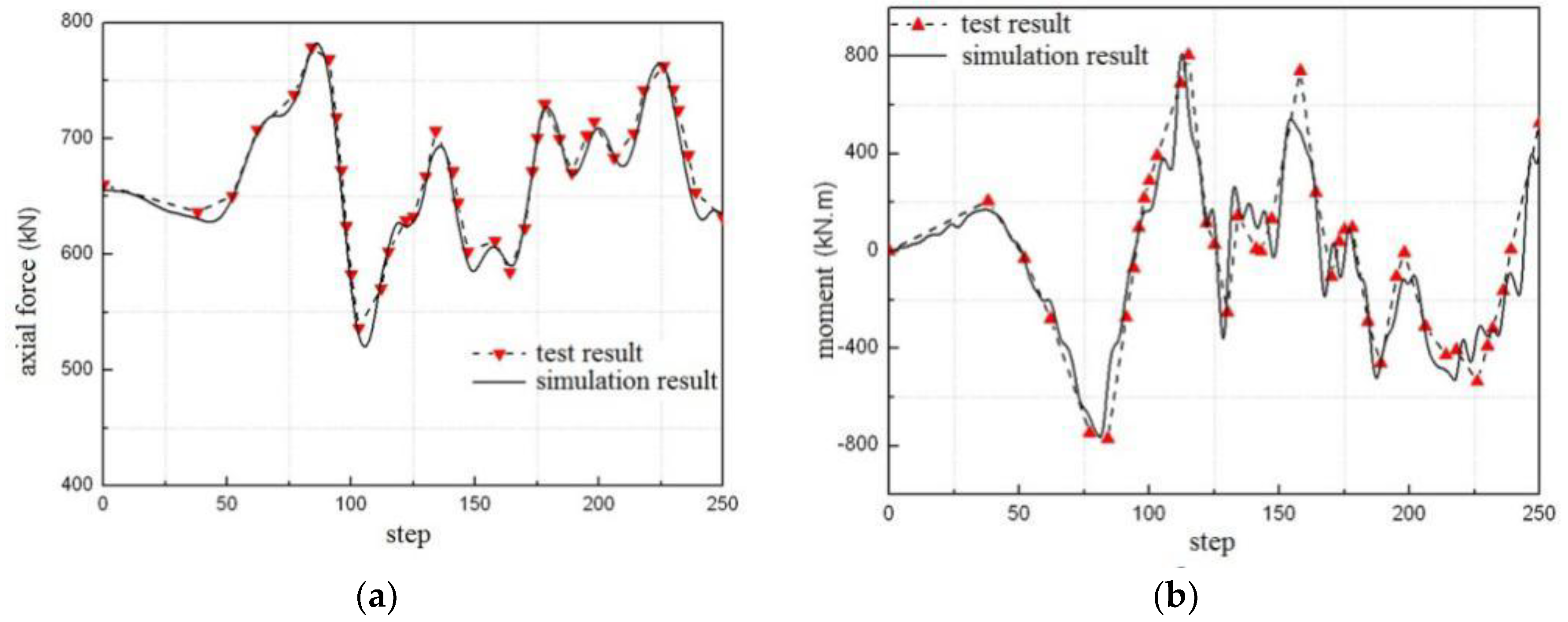
Figure 19.
The comparison curves of the internal force time history between the test results and the simulation results at the 620 cm/s2 of PGA: (a) axial force at the bottom of column; and (b) bending moment at the bottom of column.
Figure 19.
The comparison curves of the internal force time history between the test results and the simulation results at the 620 cm/s2 of PGA: (a) axial force at the bottom of column; and (b) bending moment at the bottom of column.


Table 1.
Structural parameter information.
| Test Number | Number of Story | LSR of Beam–Column | PGA (cm/s2) | Number of Story for the Physical Substructure | Beam Section (mm) | Column Section (mm) |
|---|---|---|---|---|---|---|
| 1 | 3 | 0.9 | 540 | 1 | 300 × 550 × 18 × 12 | 400 × 400 × 21 × 13 |
| 2 | 4 | 1.4 | 420 | 2 | 300 × 600 × 24 × 14 | 400 × 400 × 21 × 13 |
| 3 | 5 | 1.9 | 300 | 1 | 300 × 700 × 24 × 12 | 400 × 400 × 21 × 13 |
| 4 | 6 | 0.8 | 180 | 1 | 300 × 500 × 20 × 14 | 400 × 400 × 21 × 13 |
| 5 | 7 | 1.3 | 55 | 1 | 300 × 600 × 22 × 14 | 400 × 400 × 21 × 13 |
| 6 | 8 | 1.8 | 580 | 3 | 300 × 700 × 22 × 12 | 400 × 400 × 21 × 13 |
| 7 | 9 | 0.7 | 460 | 1 | 300 × 500 × 17 × 12 | 400 × 400 × 21 × 13 |
| 8 | 10 | 1.2 | 340 | 3 | 350 × 550 × 22 × 14 | 400 × 400 × 21 × 13 |
| 9 | 11 | 1.7 | 220 | 1 | 450 × 800 × 28 × 16 | 500 × 500 × 28 × 18 |
| 10 | 12 | 0.6 | 100 | 1 | 450 × 550 × 22 × 14 | 500 × 500 × 28 × 18 |
| 11 | 13 | 1.1 | 620 | 3 | 450 × 650 × 28 × 18 | 500 × 500 × 28 × 18 |
| 12 | 14 | 1.6 | 500 | 2 | 450 × 800 × 26 × 16 | 500 × 500 × 28 × 18 |
| 13 | 15 | 0.5 | 380 | 1 | 400 × 500 × 24 × 16 | 500 × 500 × 28 × 18 |
| 14 | 16 | 1 | 260 | 1 | 450 × 600 × 31 × 18 | 500 × 500 × 28 × 18 |
| 15 | 17 | 1.5 | 140 | 1 | 450 × 800 × 24 × 16 | 500 × 500 × 28 × 18 |
Table 2.
The test results for the steel material performance.
| Theoretical Thickness of Steel Plate (mm) | Real Thickness of Steel Plate (mm) | Yield Strength (Mpa) | Elasticity Modulus (105 Mpa) | Ultimate Strength (Mpa) |
|---|---|---|---|---|
| 7 | 6.8 | 220.5 | 2.02 | 390.4 |
| 10 | 9.85 | 202.3 | 1.90 | 323.2 |
| 12 | 10.5 | 216.0 | 2.04 | 345.6 |
| 16 | 15.7 | 206.5 | 1.91 | 339.6 |
Table 3.
Relative errors of the internal force at the peak of with various peak accelerations.
| Peak Acceleration (cm/s2) | Axial Force at the Bottom of the Column | Bending Moment at the Bottom of the Column | Bending Moment at the End of Beam |
|---|---|---|---|
| 310 | 2.5% | 3.7% | 6.1% |
| 620 | 6.7% | 9.3% | 4.0% |
© 2018 by the authors. Licensee MDPI, Basel, Switzerland. This article is an open access article distributed under the terms and conditions of the Creative Commons Attribution (CC BY) license (http://creativecommons.org/licenses/by/4.0/).
Share and Cite
MDPI and ACS Style
Chen, Z.; Yan, X.; Wang, H.; Zhu, X.; Spencer, B.F. Substructure Hybrid Simulation Boundary Technique Based on Beam/Column Inflection Points. Sustainability 2018, 10, 2655. https://doi.org/10.3390/su10082655
AMA Style
Chen Z, Yan X, Wang H, Zhu X, Spencer BF. Substructure Hybrid Simulation Boundary Technique Based on Beam/Column Inflection Points. Sustainability. 2018; 10(8):2655. https://doi.org/10.3390/su10082655
Chicago/Turabian StyleChen, Zaixian, Xueyuan Yan, Hao Wang, Xingji Zhu, and Billie F. Spencer. 2018. "Substructure Hybrid Simulation Boundary Technique Based on Beam/Column Inflection Points" Sustainability 10, no. 8: 2655. https://doi.org/10.3390/su10082655
Note that from the first issue of 2016, this journal uses article numbers instead of page numbers. See further details here.