Synthetic Pollutograph by Prediction Indices: An Evaluation in Several Urban Sub-Catchments

Abstract

A generalized methodology applicable to any urban sub-catchment to calculate the pollution curve due to combined sewer overflows would help to implement integrated management policies to reduce urban impacts on the environment. An existing methodology to predict the pollutographs associated to rainfall events is tested in five different sub-catchments with very different pluviometry. Ninety-three rainfall events have been considered by measuring the in-sewer turbidity along the runoff episodes. Such data is then evaluated to obtain two prediction indices: the time to peak of pollutograph I_TPP, and the maximum turbidity concentration I_CMAX. These indices may be used with linear regressions to calculate the characteristics of pollutographs, such as the time to the peak, TPP, the maximum concentration of turbidity, C_MAXtb, and the time to descent, TDP. These parameters allow to estimate the pollutographs of a sub-catchment. The comparison between pollutographs measured in the Ensanche sub-catchment and those calculated with the methodology shows a good agreement in terms of the root mean square deviation between samples and estimated values with the model proposed. Hence, the methodology could be a key way to find synthetic pollutographs for any sub-catchment.

1. Introduction

Combined sewer overflows (CSOs) constitute a source of diffuse urban pollution that impacts the environment and human health. The CSO systems are referred to in Directive 91/271/EEC, the Urban Waste Water Treatment Directive (UWWTD), and indirectly in others, such as the Water Framework Directive (WFD, 2000/60/EC), Bathing Water Directive (BWD, 2006/7/EC), the Groundwater Directive (GWD, 2006/118/EC), and the Environmental Quality Standards Directive (EQS, 2008/105/EC). These European Union (EU) directives require that Member States include measurements in their plans for the conservation or restoration of the environment. The UWWTD sets mandatory limits for specific polluting substances and specific requirements for storm water overflows. These legislations require the monitoring and the assessment of emissions to water that should be addressed through combined sewer overflow integrated planning [1,2,3,4,5].

To achieve this, the knowledge on storm water quality is needed based on time-continuous sampling campaigns and laboratory analyses to understand the dynamic of pollutographs. Time-continuous water quality monitoring based on turbidity measurements offer correlations between several pollutants, such as particles and organic matter [6,7,8,9,10,11]. Other methods, like ultraviolet–visible (UV–VIS) spectrometric sensors, present better correlations between spectrophotometric measurements and organic matter and nitrogen. In-sewer sensors are interesting and useful tools to measure water pollution during dry and wet weather conditions and long-term operational scenarios [12].

Once field data is available, the next step is to establish accurate models to simulate runoff pollution. Here we can distinguish, on the one hand, the physically-based models, that generally simulate surface accumulation, wash-off, sediment erosion, and pollutant transport in sewer systems [13,14]. In case of physically-based models Di Modugno et al. [15] present pollution cumulative curves as a function of total runoff volume, also named M(V) curves, and the adjustment of pollution mobilization to a build-up and wash-off model in Storm Water Management Model (SWMM) software [13]. Others like Willems [16] study uncertainty associated to quality models that are integrated in hydraulic models.

On the other hand, are those stochastic methods where different parameters of the pollutograph curve, like the maximum turbidity concentration C_MAXtb, or other global parameters in combined sewer overflows, like the event mean concentration of a pollutant, EMC, among others, have been adjusted by statistical approaches from samples taken during rainfall events [17,18,19,20,21,22,23,24,25]. Lee and Bang [17] present M(V) curves for different events in nine sub-catchments. Additionally, they calculate the EMC, and propose a linear regression to obtain the annual rate of pollution associated to a sub-catchment. Nazahiya et al. [18], from urban runoff samples in a small catchment, analyze EMC and M(V) curves, too. Gupta and Saul [19] present specific regression relationships to predict the first flush load of suspended solids in a combined sewer flow for pollutant-suspended solids, SS. LeBoutillier and Putz [20] also propose global volume indicators of pollution per event by linear regressions. Gromaire et al. [21] compare different pollutants, like heavy metals, at different sub-catchments with a predomination of different surfaces, such as roofs, yards, or streets. They calculated the total volume of pollution and concluded that erosion of in-sewer pollutant stocks was found to be mainly of particles and of organic matter in wet weather runoff flows. Lau et al. [22] studied the frequency of volume of CSO spills as an indicator of receiving water pollution impact. Francey [23] presents global event parameters and also the maximum event concentration of pollutant, C_MAX. Harremoës [24] checks that EMC of pollutants adjusts to a log-normal function as a function of rainfall volume. Logarithmic overall mean concentration plus standard deviation for characteristic land uses and characteristic properties of the sewer system are proposed by this author to be a key factor of pollution. Suarez and Puertas [25] present the adjustment of C_MAX and EMC to a log-normal base 10 function for different pollutants, like chemical organic matter, COD, and SS. In summary, authors [17,18,19,20,21,22,23,24,25] presented several statistics methods to characterize pollution associated to overflows from sewer networks that are not still addressed to build the pollutograph associated to each rainy event. For instance, the M(V) curves describe how pollution is distributed along the episode in percentage. However, these curves do not quantify the pollution mobilized with time. The first attempts to obtain a pollutograph associated to a rainy event based on statistics were presented by Garcia et al. [26]. From this curve of pollution, it would be possible to evaluate the efficiency of techniques to reduce pollution such as construction of ponds.

Stochastic models allow forecasting the water pollution parameters associated to CSOs. The possibility of application stochastic models to any sub-catchment with enough accuracy is an important objective, taking into account the large differences observed in pollution patterns at different sub-catchments. Definitely, achieving a generalized methodology for defining synthetic pollutographs would be very helpful in the CSOs integrated planning [1,3,22].

If we look into the prediction of design storms in urban catchments, the depth-duration-frequency (DDF) curves at each precipitation station point are widely used [27]. From this, the construction of a synthetic unit hydrograph is a useful and implemented tool for runoff studies [28,29]. For instance, the Soil Conservation Service (SCS) and Clark unit hydrographs are used in ungauged watersheds with little available information. Those methods only need three parameters: the area of the catchment, its time of concentration, and the rainfall characteristics. These techniques enable the estimation of the runoff at any outfall point of the sub-catchments with good accuracy despite the sparse input data. In the same way, being able to have a generalized catchment-independent methodology that would allow obtaining the pollution curve over time would be of great help when establishing CSO integrated planning.

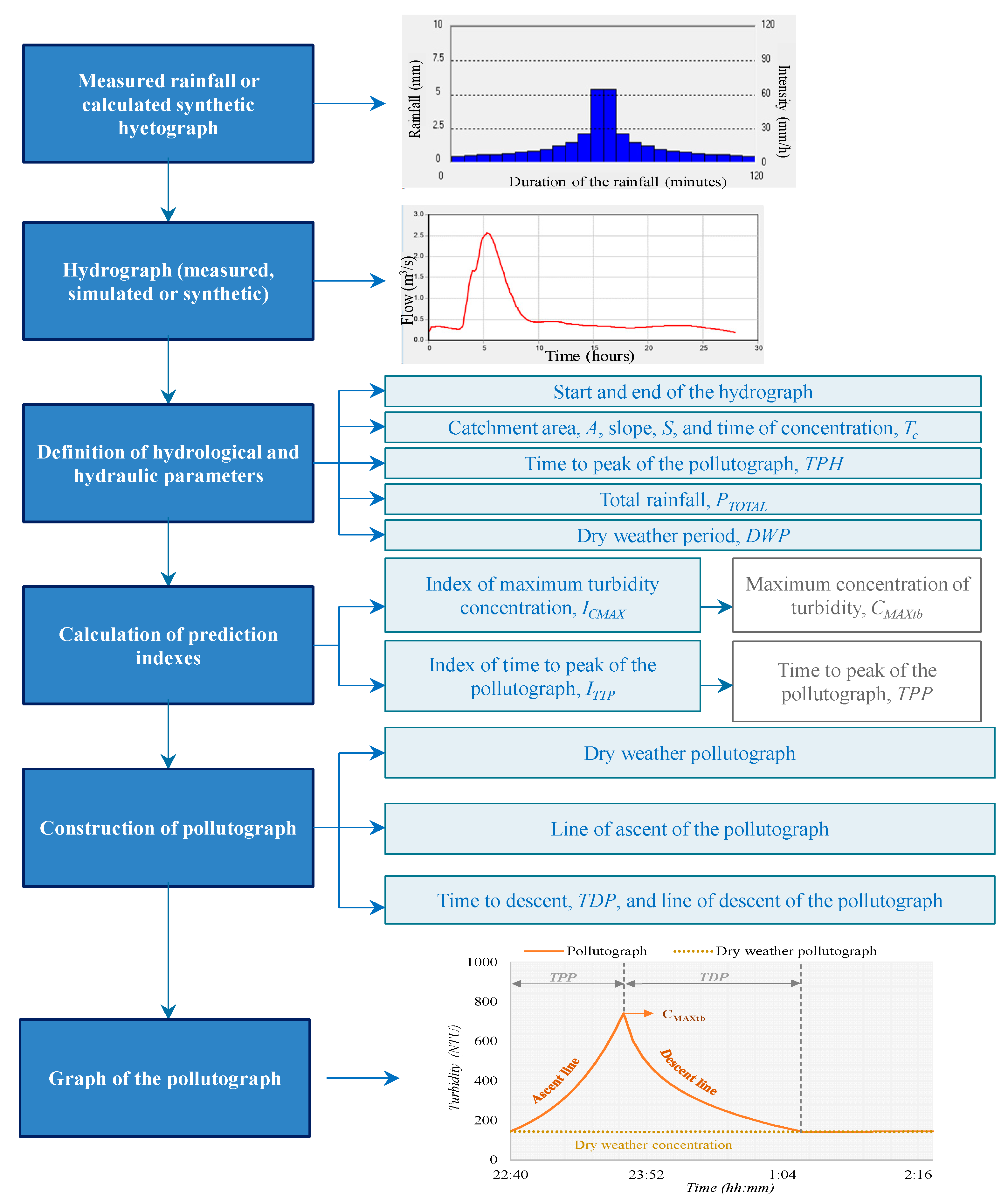
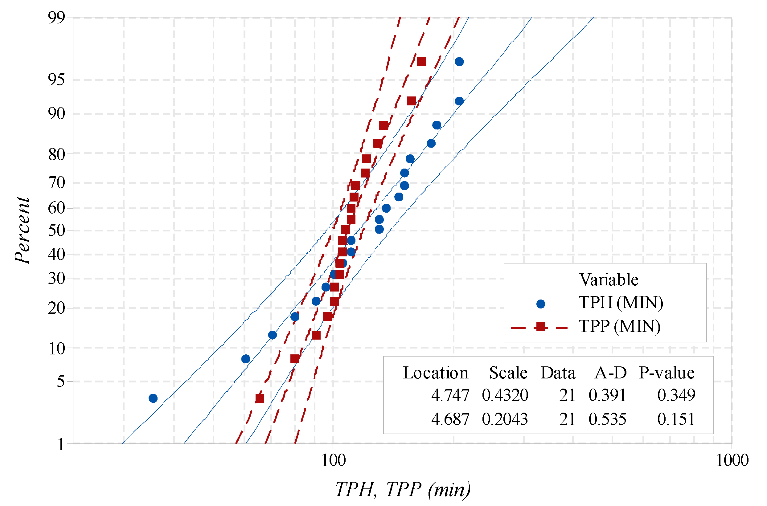
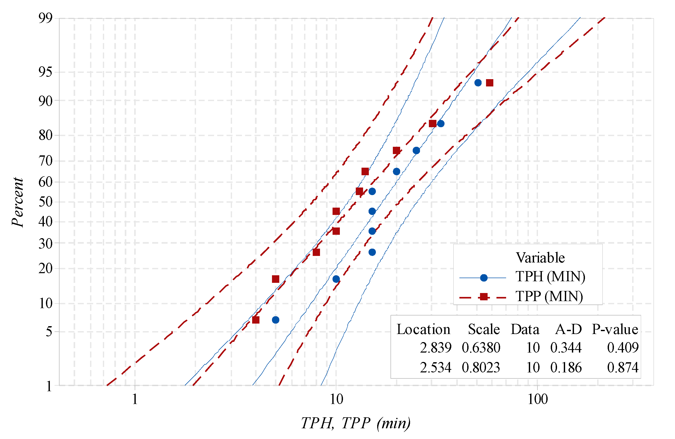
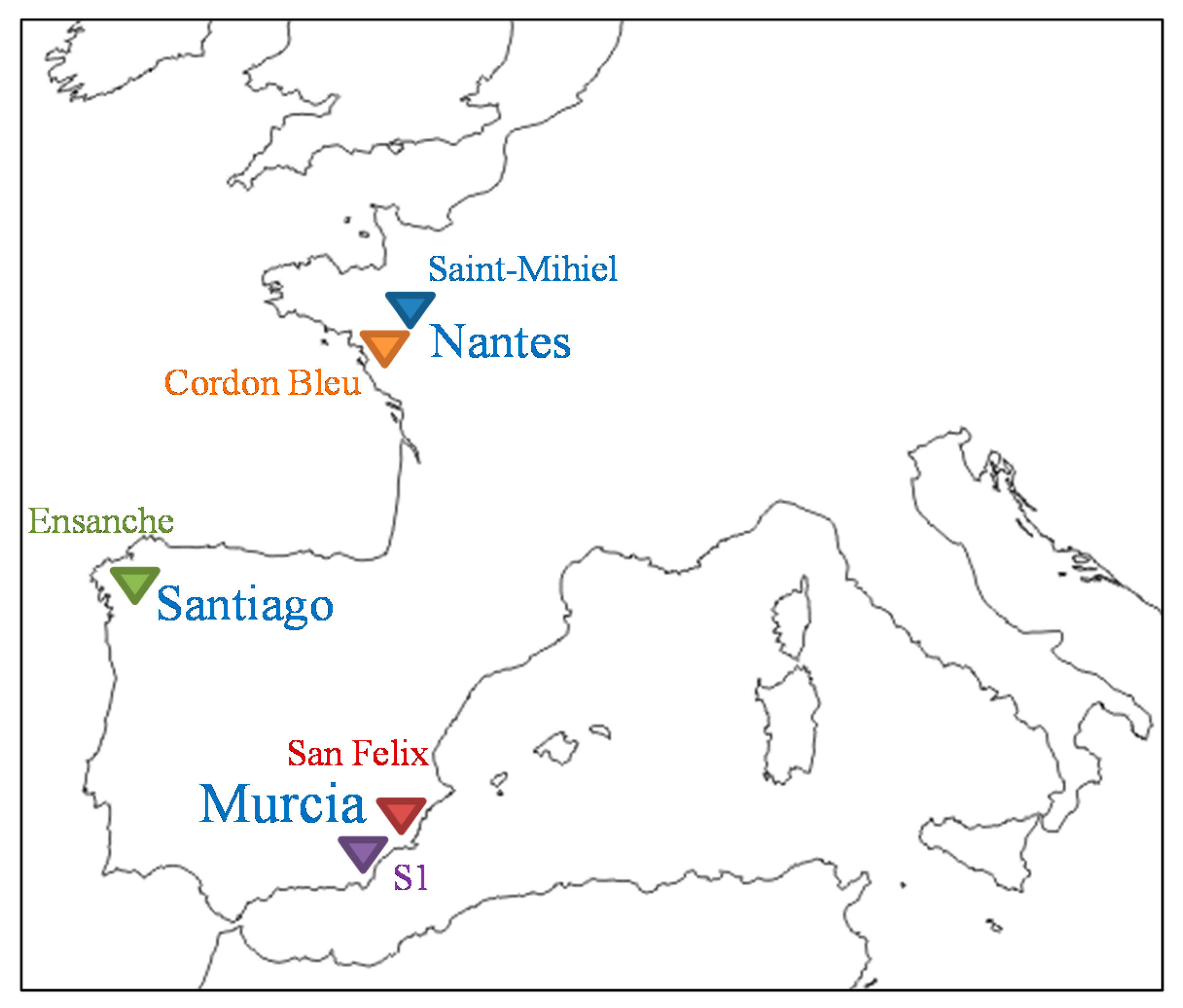
Based on time-continuous turbidity measurements in two urban sub-catchments, García et al. [26] proposed a stochastic methodology which allowed the prediction of the event maximum turbidity concentration (C_MAXtb), the time to the peak of the pollutograph TPP, and the time to the descent of pollutograph TDP, from intermediate stochastic predictor indices. This procedure is summarized in Figure 1. In this work, the statistical prediction indices proposed by García et al. 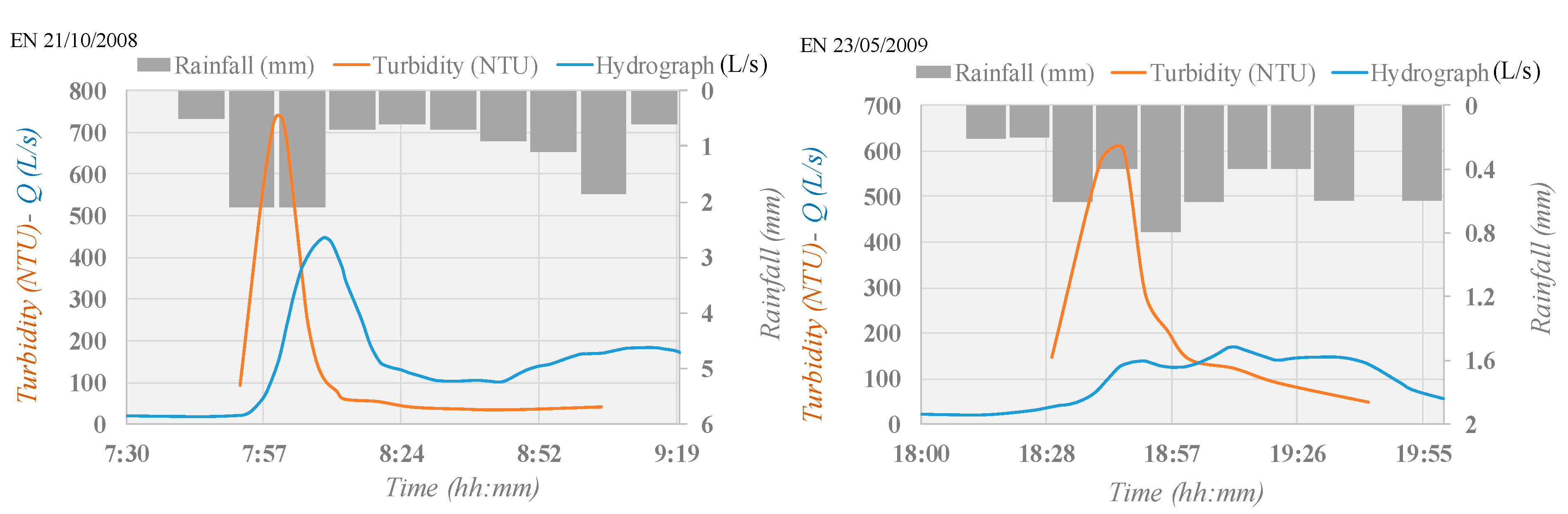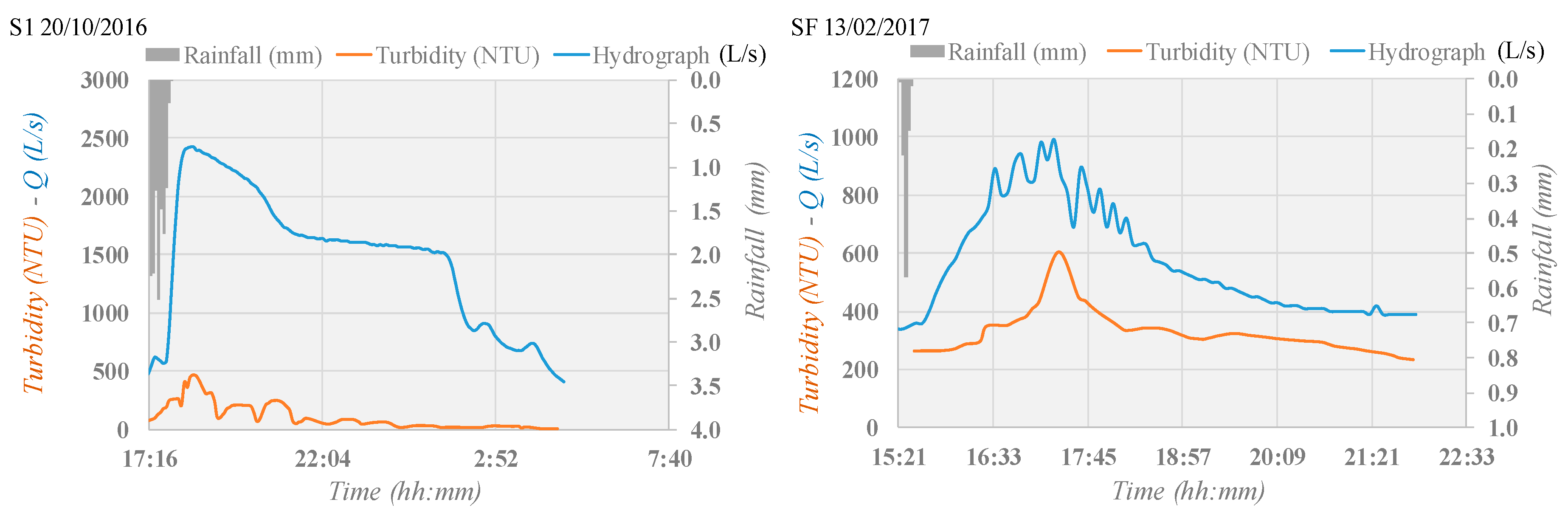[26] are evaluated for different sub-catchments: Saint-Mihiel and Cordon-Bleu, from data collected in Hannouche [30]; Ensanche, from data of Del Río [6]. Moreover, three new rainfall events were considered in sub-catchments S1 and San Félix, besides the events from previous works [26]. A total of ninety three events were considered in present work, of which seventy four are new, and the others were considered from previous adjustments of the proposed stochastic model in García et al. [26].

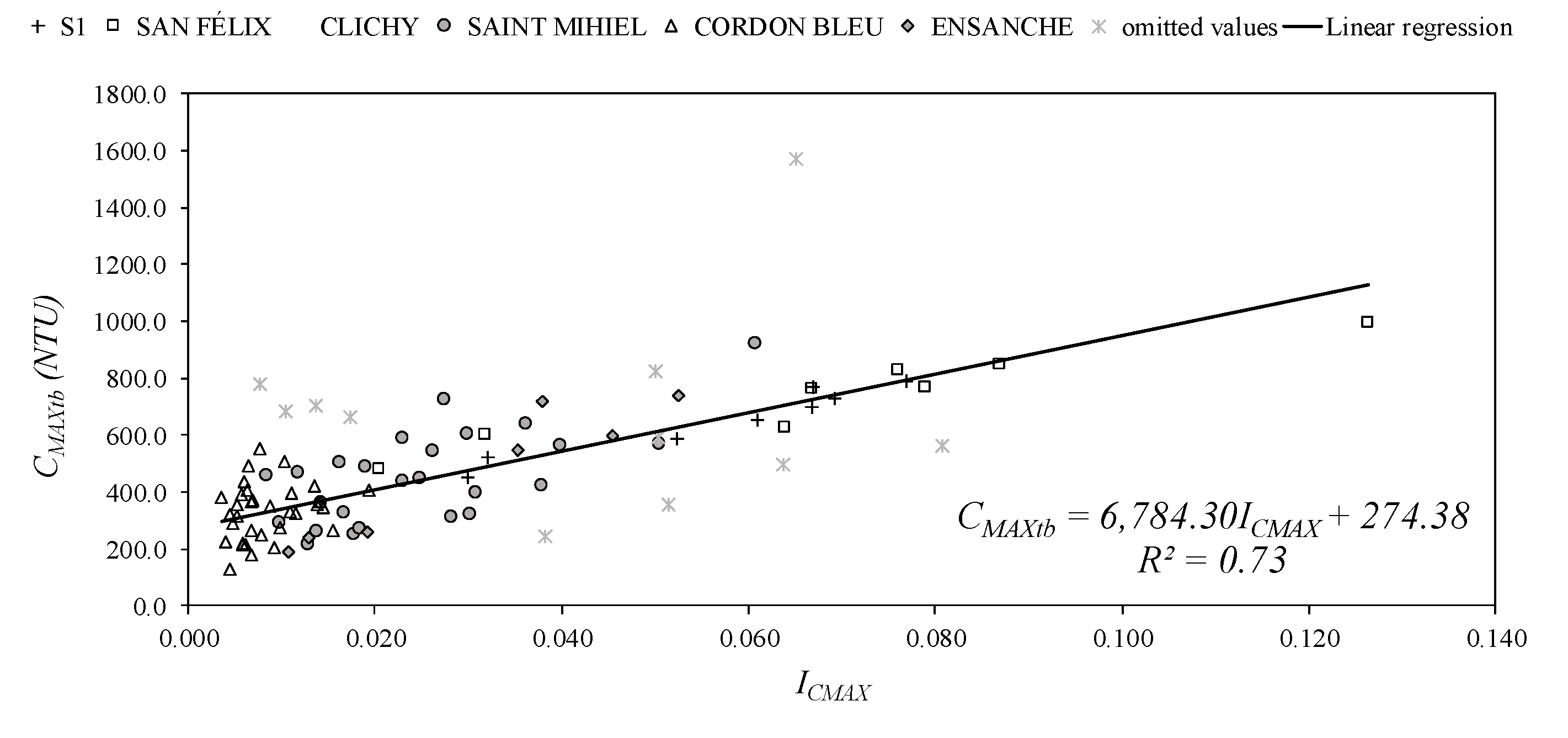
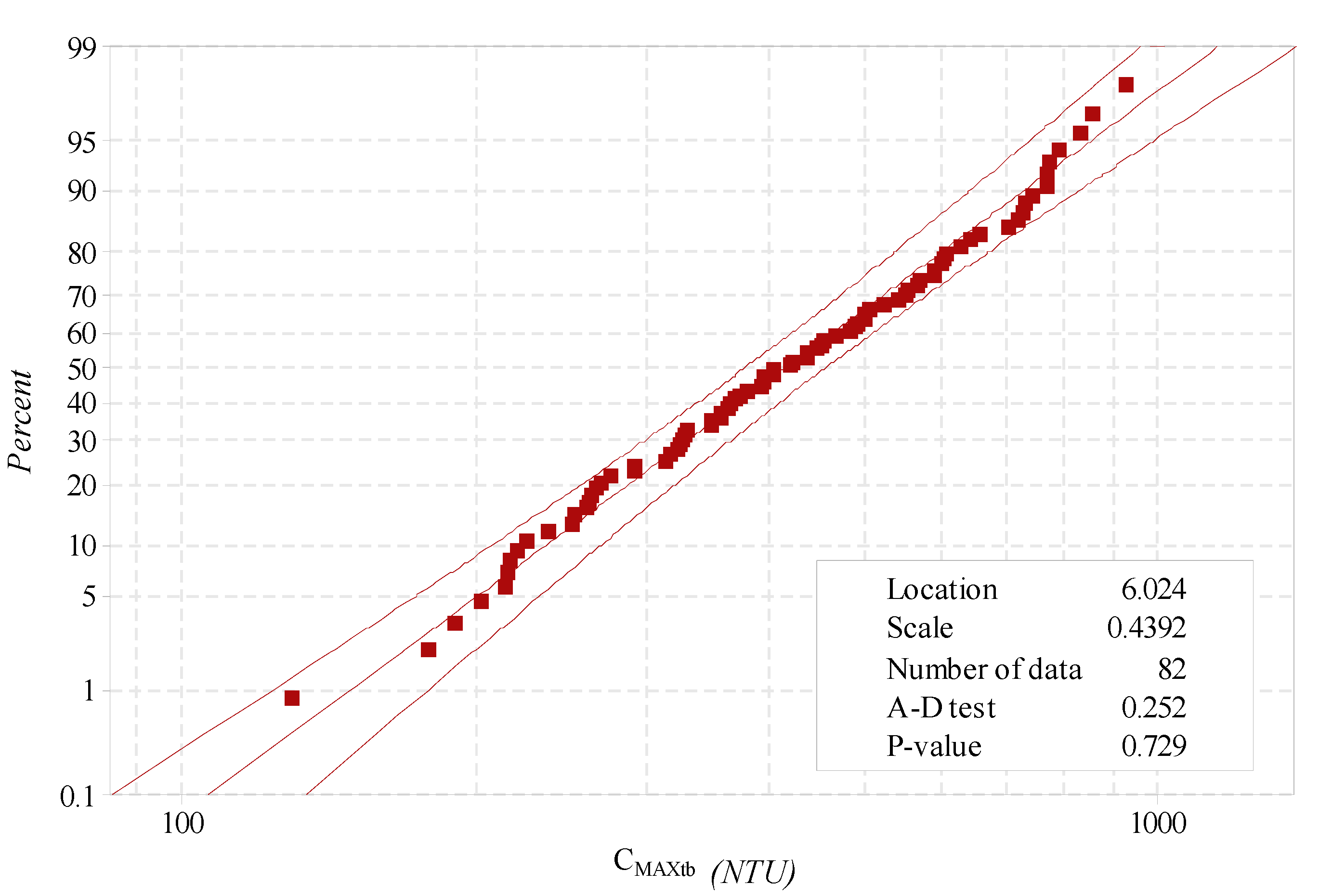
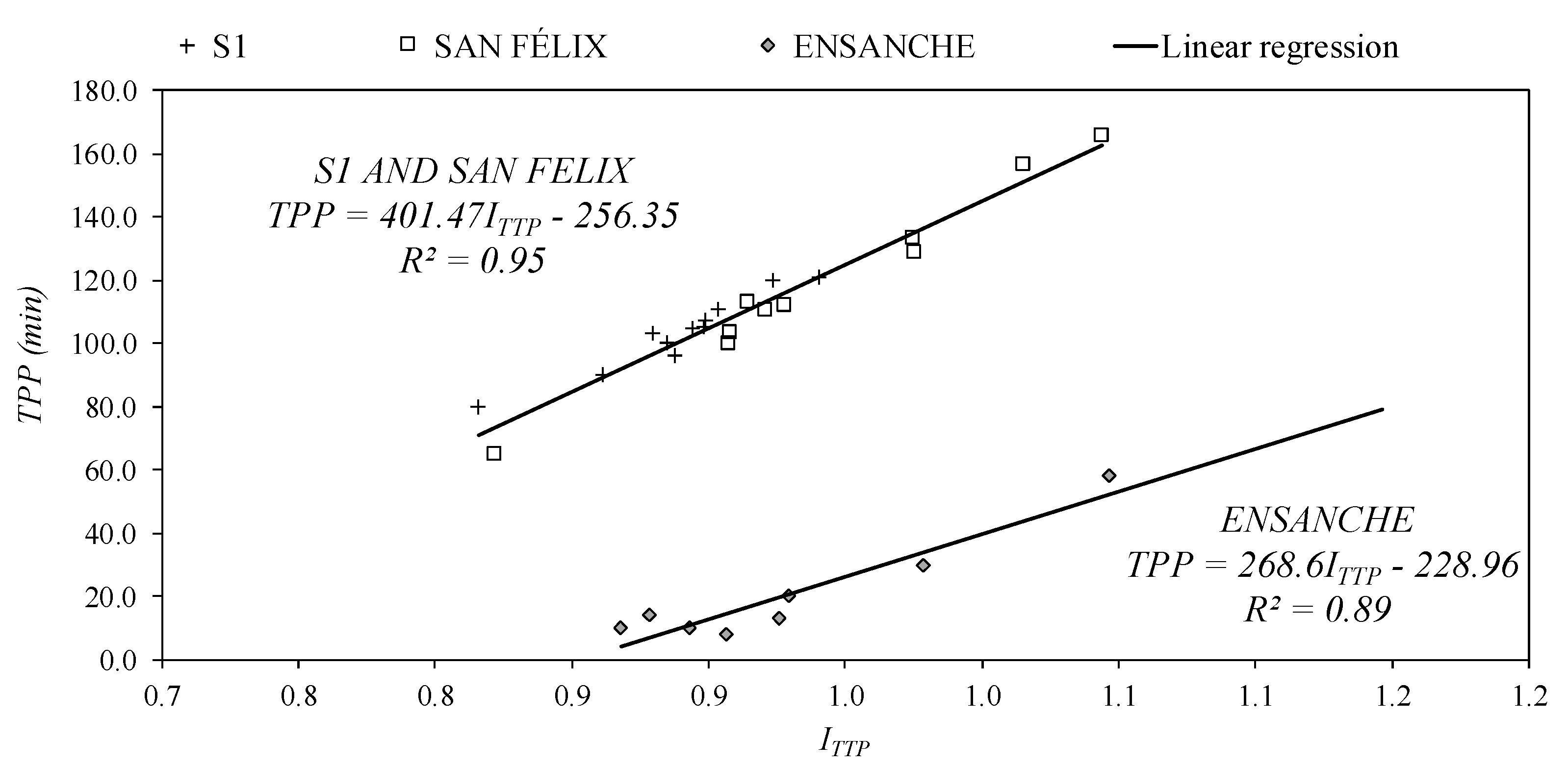
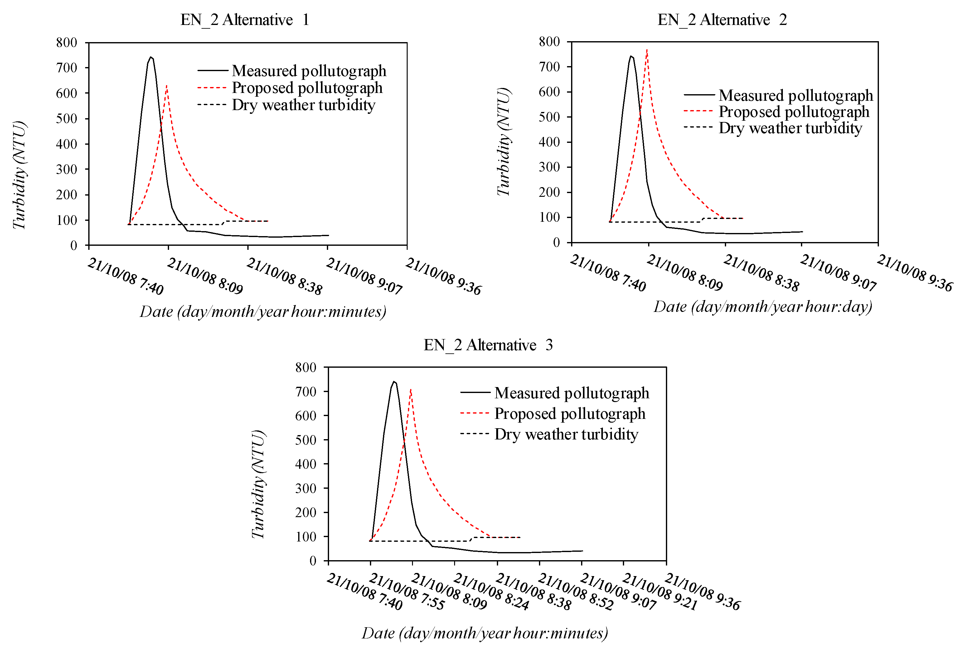
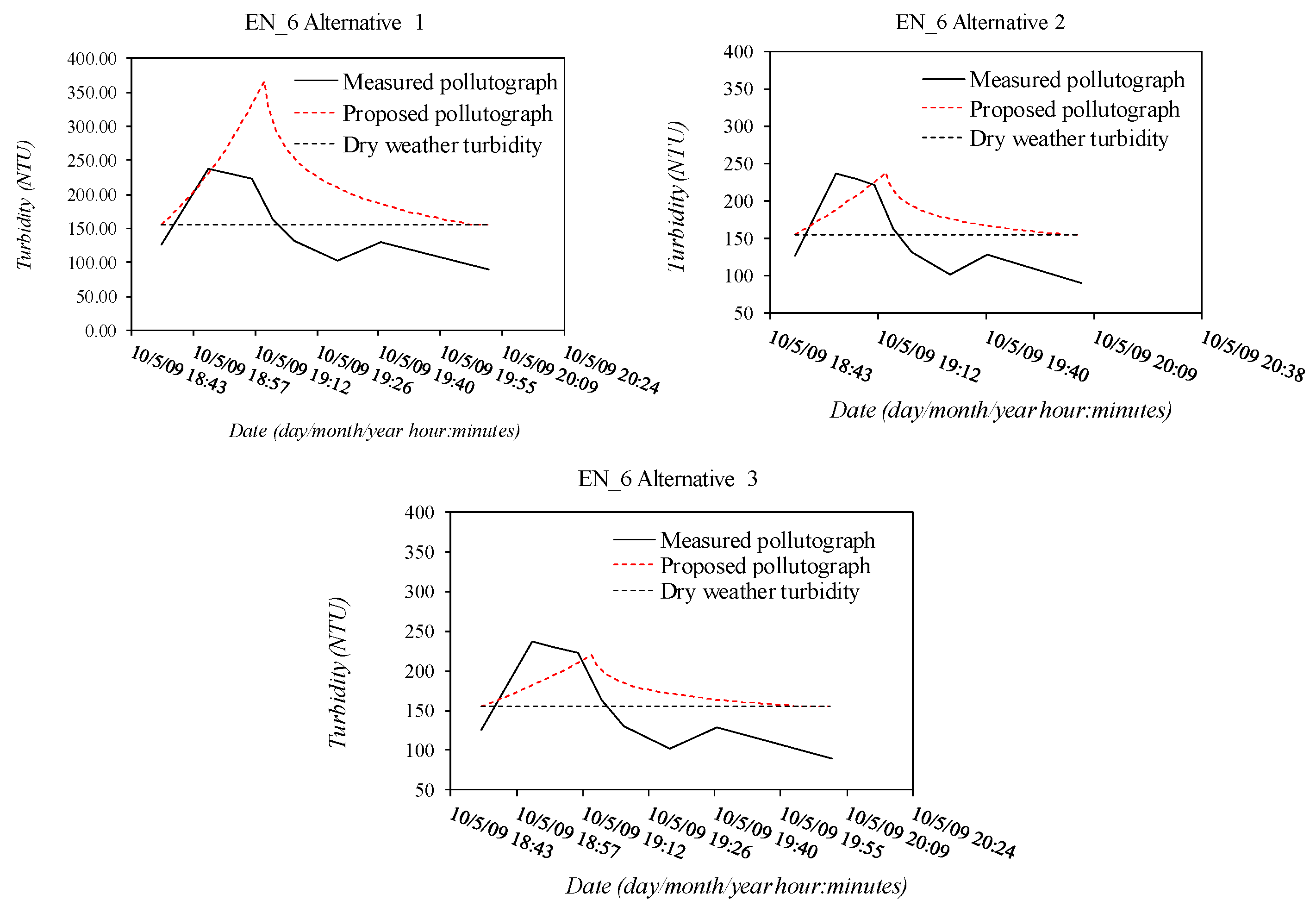
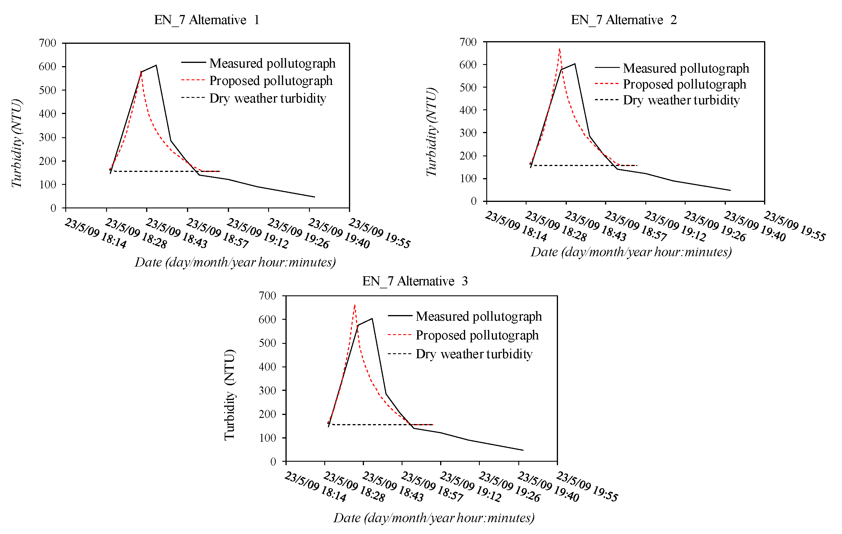
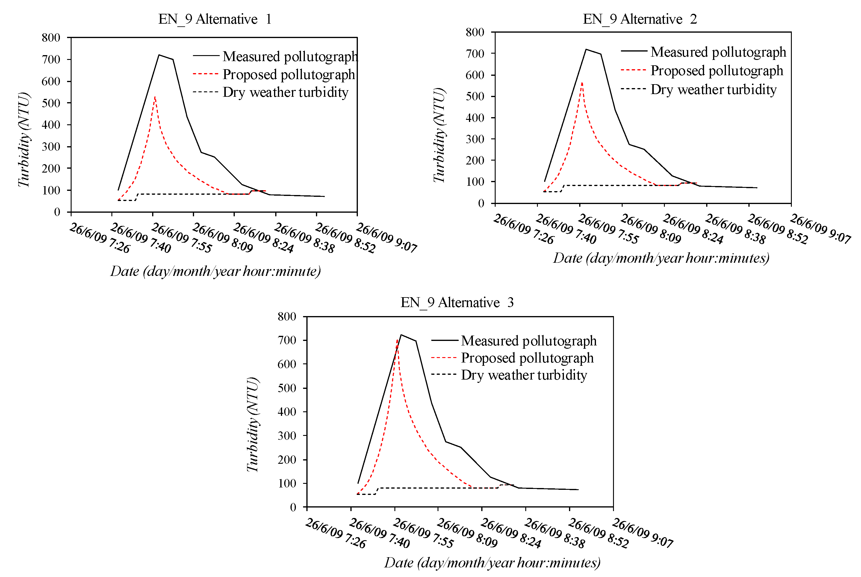
Discussion of the adjustment achieved with the index of maximum turbidity concentration, I_CMAX, in case of the five sub-catchments, is presented. In the case of the stochastic predictor index of the time to peak of the pollutograph, I_TPP, due to the information available, is presented in the case of sub-catchments Ensanche [6], S1, and San Félix [26]. Finally, the measured pollutographs for rainfall events in the Ensanche sub-catchment [6] are also compared with those obtained with the proposed methodology.

2. Materials and Methods

2.1. Description of Sub-Catchments Areas

2.1.1. San Félix and S1 at Murcia, South East of Spain

Murcia is a southeastern Spanish city with an equivalent population of 525,027 (Figure 2). This study site included two urban sub-catchments, called San Félix and S1. Both catchments were residential areas, their impervious areas being 47% and 21%, respectively (

Table 1. S1 and San Félix sub-catchments descriptions.

Sub-Catchment	San Félix	S1
Area of catchment (km2), A	14.89	47.53
Population density (inh/km2)	14,250	2685
Ratio of imperviousness (m2/m2)	0.47	0.21
Mean slope (m/m), S	0.0043	0.0013
Catchment flow length (km), L	10.75	17.00
Length combined sewerage (km)	513.15	616.84

). The sewer system is combined, incorporating storm water.

2.1.2. Ensanche Sub-Catchment at Santiago de Compostela Sub-Catchments, Northwest Spain

The Ensanche sub-catchment is located in Santiago de Compostela (Galicia–Spain). All the information of this sub-basin was obtained from Del Río [6]. It is one of the 13 main sub-catchments of the city’s sanitation and drainage system. Ensanche has a predominantly unitary urban sewer network that serves an approximate population of 25,000 inhabitants and its approximate surface area is 38 ha. The instrumentation equipment could not be located at the outfall point of the sub-catchment network. However, it covers approximately half of the total area of Ensanche (around 20 ha and a population of 13,000 inhabitants).

Table 2. Ensanche sub-catchment description (Del Río [6]).

Sub-Catchment	Ensanche
Area of catchment (km2), A	0.20
Population density (inh/km2)	65,000
Ratio of imperviousness (m2/m2)	-
Mean slope (m/m), S	0.0042
Catchment flow length (km), L	1.40
Length combined sewerage (km)	-

shows the main details of the sub-catchment.

2.1.3. Saint-Mihiel and Cordon-Bleu Sub-Catchments, South of France

The Saint-Mihiel sub-catchment has an area of 100 ha and it is located upstream of the central area of the city of Nantes (Figure 2). It is entirely unitary. The Cordon-Bleu sub-catchment is much larger (5000 ha) and it is located downstream of the main collector of the Nantes agglomeration (right bank of the Loire River) near to the Tougas wastewater treatment plant and serving approximately 500,000 equivalents inhabitants. Although only half sub-catchment is unitary, the measurement point is located in an accessible unitary manifold of ovoid section. The slope of this sewer is 0.04%.

Table 3. Saint-Mihiel and Cordon-Bleu sub-catchments description (Hannouche [30]).

Sub-Catchment	Saint-Mihiel	Cordon-Bleu
Area of catchment (km2), A	1.00	50.00
Population density (inh/km2)	-	10,000
Ratio of imperviousness (m2/m2)	-	-
Mean slope (m/m), S	0.0010	0.0004
Catchment flow length (km), L	2.50	25.00
Length combined sewerage (km)	-	-

shows the details of the two sub-catchments obtained by Hannouche [30].

2.2. Monitoring Equipment in the Evaluated Sub-Catchments

S1 and San Félix sub-catchments have a water gauge to continuously monitor the flow, while two different probes measure turbidity, conductivity, and temperature. The turbidity data is obtained with an infra-red nephelometric turbidimeter Endress+Hauser CUS 42 measuring at a wavelength of 880 nm according to the standard NF EN 27027, associated to a data logger. A backwash process with clear water is automatized each hour to avoid disturbing measurements. Turbidimeters are calibrated with formazine solution. A technique for the removal of these outliers has been implemented.

In the Ensanche sub-catchment, a continuous sampler was installed with intervals of five and ten minutes between samples. This also allowed the characterization of the turbidity of the sample in Nephelometric Turbidity Units, NTUs. Flow depth, flow velocity, and flow meters were installed at the measurement point located in the Ensanche sub-catchment. Ten rain events with values of turbidity are available (Del Río [6]).

In Saint-Mihiel and Cordon-Bleu sub-catchments the rainfall was measured with the nearest rain gauges. Time-continuous turbidity was also measured during dry and wet weather by a turbidity probe in Formazin Attenuation Units, FAUs. In rainy weather in Cordon-Bleu, 35 events were sampled to establish total suspended solids TSS/turbidity relationships. For Saint-Mihiel, 27 rain events were sampled for SS/turbidity relationships. Detailed values are collected in Hannouche [30]. Hydrological characteristics of the rainfall events at both sites, like precipitated height, previous dry time, rain duration and maximum intensities in 5 and 60 min, Imax₅ and Imax₆₀ are also included in this work. Some hydraulic parameters, such as the time to peak of the hydrograph, TPH, could not be obtained due to the lack of instrumentation to measure the flow.

In case of turbidity determinations, the optical method of measurement for FAU is different than the NTU method. However, all measurements were calibrated with formazine solution. This allowed for considering that the value for each of these units are equivalent.

In Figure 3, the measured rainfall in intervals of five minutes, the estimated hydrograph and the measured time-continuous turbidity are presented for two novel events in sub-catchments S1 and San-Félix. Figure 4 shows the measured rainfall, measured flow rate and turbidity calculated by sample analysis in the Ensanche sub-catchment in two events, as presented in Del Rio [6]. Remarkable differences in event duration are observed due to the concentration time of each sub-catchment: 15 min in the Ensanche sub-catchment; 193.75 min in the S1 sub-catchment; and 87.14 min in the San Félix sub-catchment.

3. Results and Discussion

3.1. Variables Definition from Wet Weather Measured Events

Table 4. Variables measured at each sub-catchment in wet weather events.

	Sub-Catchment	S1	San_Félix	Saint-Mihiel	Cordon-Bleu	Ensanche
	Years of study	2014–2017	2014–2017	2002–2007	1998–2006	2008–2009
	Number of events	11	10	27	35	10
Hydrology	PTOTAL (mm)	X	X	X	X	X
	Imean (mm/h)	X	X	X	X	X
	Imax5–10 (mm/h)	X	X	X	X	X
	DWP (days)	X	X	X	X	X
	A (ha)	X	X	X	X	X
	TC (h)	X	X	-	-	X
Hydraulic	Qmax (L/s)	X	X	-	-	X
	Qmean (L/s)	X	X	-	-	X
	TPH (min)	X	X	-	-	X
Quality	CMAXtb (NTU)	X	X	X	X	X
	EMCtb (NTU)	X	X	X	X	X
	TPP (min)	X	X	X	X	X

Where X represents that this information is available, P_TOTAL is the total event rainfall, I_mean is the mean rainfall intensity, I_max5–10 is the maximum 5, 10 min rainfall intensity, DWP is the proportion of consecutive dry weather days previous to the event in the last month, T_C is the time of concentration of urban catchment, Q_max is the maximum event inflow, and Q_mean is the mean event inflow.

summarizes the required variables for the calculation of the predictor indices and the application of the methodology [26]. These data have been obtained from [6,26,30].

3.2. Pollution Prediction Indices. Statistical Model

The maximum concentration index I_CMAX, and the time to peak of the pollutograph index I_TPP are calculated in order to adjust afterwards (i) the maximum concentration of turbidity during each event, C_MAXtb; and (ii) the time elapsed from the beginning of the event until the maximum peak of the pollutograph TPP.

3.2.1. Maximum Concentration Index I_CMAX

The maximum concentration index I_CMAX arises with the objective of estimating the maximum concentration of turbidity C_MAXtb, from predictor variables quantified in rainfall events. Together with the I_TPP, they allow the estimation of both the magnitude of the pollutograph and the location in time of the highest turbidity. The equation for I_CMAX was previously defined as [26]:

$$I_{CMAX}={\left(\frac{P_{TOTAL}}{P_{{TOTAL}_{ANNUAL}}}S\right)}^{0.3}{\left(\mathrm{DWR}\right)}^{0.3}{F}_{shape}$$

(1)

where P_TOTAL is the rainfall volume of each event (mm); P_TOTALANNUAL is the total precipitation expected in a year, adopting 350 mm for the cases of sub-catchments S1 and San Félix, 800 mm for Saint-Mihiel and Cordon-Bleu, and 1300 mm for the Ensanche sub-catchment; DWR is the proportion of consecutive dry weather days previous to the event in the last month (DWP/30); and S is the mean slope of the sub-catchment (m/m).

Equation (1) is dimensionless and represents the power of the event. It is multiplied by the time without precipitation, accounting for the effect of the possible sedimentation during the dry weather period. F_shape is a shape factor of the sub-catchment defined as:

$$F_{shape}=\frac{10A}{L^2}$$

(2)

where A is the area of the sub-catchment (km²) and L is the catchment flow length (km).

Table 5. Catchments’ shape factors.

Sub-Catchment	Slope (m/m)	Sub-Catchment Flow Length, L (km)	Sub-Catchment Area, S (km2)	Fshape (-)
S1	0.0013	17.00	47.53	1.65
San Félix	0.0043	10.75	14.89	1.29
Saint-Mihiel	0.0010	2.50	1.00	1.60
Cordon-Bleu	0.0004	25.00	50.00	0.80
Ensanche	0.0042	1.40	0.20	1.02

summarizes the shape factors obtained in the sub-catchments analyzed.

Figure 5 presents the values of I_CMAX, calculated by Equation (1) for each rainfall event, and the maximum measured turbidity in each event C_MAXtb. A linear relation between the later variable and the index is obtained through a least squares adjustment. The values are mainly explained by such a common line except for four events in sub-catchments S1 and San Félix out of their 21 events. Those different cases are due to very low precipitation episodes or anomalously high registered values for the maximum turbidity that should be studied in more depth. In Sain-Mihiel sub-catchment, two values from the 27 existing values were not considered. In the Cordon-Bleu sub-catchment, two of the thirty-five existing values were omitted. In the sub-catchment of Ensanche three of the 10 values were not used in the adjustment. To sum up, 11 cases were omitted from a total of 93. The relationship between C_MAXtb and I_CMAX fit to a line with a coefficient of determination R² = 0.73. Figure 5 also presents the values omitted from the adjustment.

Table 6. Regression parameters.

Sub-Catchment	m (Slope)	n (Intercept)	R2
S1	6678.70	269.50	0.94
San-Félix	4864.70	398.95	0.91
Saint-Mihiel	8800.30	232.79	0.45
Cordon-Bleu	5699.10	282.06	0.05
Ensanche	13,682.00	52.16	0.91
All Data	6784.30	274.38	0.73

shows the regression coefficients and the coefficient of determination obtained for each sub-catchment independently and considering all the non-omitted data.

The fitted line of the adjustment between the maximum concentration index, I_CMAX, and the maximum concentration of turbidity, C_MAXtb, is given by a linear regression:

$$C_{MAXtb}=6784.30I_{CMAX}+274.38$$

(3)

In the case of the Ensanche sub-catchment, the linear adjustment proposed in Equation (3) may be improved by using two additional alternatives: Alternative 2, i.e., adopting the regression equation presented in Table 6 considering only data of the Ensanche sub-catchment, with a coefficient of determination R² = 0.91, or the named Alternative 3, changing the power factors in Equation (1) to the values of 0.43 (first term) and 0.85 (second term), while the exponent of F_shape remains constant, reaching the following regression adjustment.

$$C_{{MAXtb}_{Ensanche}}=75,867.00I_{CMAX}+200.27$$

(4)

with R² = 0.99. These three alternatives will be evaluated in the following sections. Equation (3) and (4) could be dimensionless dividing both sides of each equation by the 90th percentile of C_MAXtb, calculated from the adjustment to a lognormal distribution of the 82 validated values of C_MAXtb. This distribution was already proposed by Suarez and Puertas [25] and by Butler and Davies [31]. This dimensionless procedure does not change the values of C_MAXtb obtained with previous Equations (3) and (4). The lognormal fit graphic of C_MAXtb values have been included in the text through Figure 6. Lognormal parameters, such as location, scale, p-value for 0.05 significance, and the Anderson–Darling statistic are presented [32]. Figure 6 includes the fitted line and the 95% confidence intervals. In summary, the 90th percentile of C_MAXtb could be used as the variable for dimensionless. Results of C_MAXtb obtained through Equations (3) and (4) by proposed dimensionless would not change the previously obtained results.

3.2.2. Time to the Peak of Pollutograph Index I_TPP

The time to the peak of the pollutograph index TPP, may be used to predict the time that elapses from the beginning of the episode until the maximum value of turbidity is achieved. It is defined from dimensionless factors [26]:

$$I_{TPP}={\left(\frac{TPH}{T_C}\right)}^{0.13}{\left(\frac{P_{TOTAL}}{P_{{TOTAL}_{ANNUAL}}}\right)}^{0.02}$$

(5)

where TPH is the time to the peak of the hydrograph that was measured in S1, San Félix, and Ensanche sub-catchments and T_c is the time of concentration of the sub-catchment. Those values were not registered in the Saint-Mihiel and Cordon Blue sub-catchments (see Table 4). In previous works [26], it was analyzed the most suitable equation to obtain the time to concentration, T_c, in urban sub-catchments with flow through sewer networks. The most suitable equation seems to be the Témez [33] equation modified for urban areas [34]. Further information about Equation (5) and the explanation of its terms is presented in [26].

Figure 7 shows the linear relationship between the time to the peak of the pollutograph index, and the time to the peak of pollutograph. A linear regression that relates the time to the peak of the pollutograph index and the time to the peak, expressed in minutes, was obtained for S1 and San Félix sub-catchments as:

$$TPP=401.47I_{TPP}-256.35$$

(6)

In the Ensanche sub-catchment, the following linear regression was obtained:

$$TPP=268.60I_{TPP}-228.96$$

(7)

For the adjustment of Equation (7), two points that had a value of time to peak less than ten minutes were omitted for the adjustment.

In the same way as previous section, Equations (6) and (7) may be dimensionless dividing both sides of each equation by a variable of time to peak of pollutograph. The lognormal distribution is adjusted for the variables TPP and TPH for S1 and San-Félix grouped sub-catchments. An independent adjustment is obtained for the Ensanche sub-catchment. Figure 8 and Figure 9 present the fit of TPP and TPH values to a lognormal distribution. Lognormal parameters such as location, scale, p-value for 0.05 significance, and the Anderson–Darling statistic are also presented [32]. The figures include the fitted line and the 95% confidence intervals. In summary, the 90th percentile of TPP could be used as the variable for dimensionless specifically for each sub-catchment. These operations would not change the results obtained in Equations (6) and (7) of TPP.

3.3. Definition of Pollutographs from Prediction Indices

Once the TPP and the C_MAXtb have been calculated, to complete the pollutograph it is necessary to know the ascent and descent curve and the time to descent of pollutograph, TDP. According to García et al. [26], the line of ascent may be adjusted with the following exponential equation:

$$C_a={\mathrm{ab}}^x=C_0{\left[{\left(\frac{C_{MAXtb}}{C_0}\right)}^{\frac{1}{N_a}}\right]}^n$$

(8)

where N_a is the number of intervals of 5 min in which the ascent time is divided; n indicates the interval (0 ≤ n ≤ N_a) in units of five minutes; and C_a and C₀ are the turbidity values at each interval n and at the beginning of the pollutograph, respectively (measured in NTU). The value of C₀ is assumed as the dry weather value at the beginning of the episode.

The time to the descent of pollutograph TDP, is defined as the time interval between the instant of the maximum concentration and the time when the concentration reaches dry weather values. The time to the descent of the pollutograph value has been adjusted for each sub-catchment showing a linear relationship with pollutograph time to the peak. The adjustment of TDP for the Ensanche sub-catchment is given by:

$$\mathrm{ENSANCHE}\to TDP=10TPP-5$$

(9)

where TPP and TDP are expressed in minutes in this equation.

In the same way as in previous sections, Equation (9) could be dimensionless by considering the 90th percentile of TPP, not introducing modifications in the results.

The descent line of the pollutographs may be adjusted to a logarithmic function as:

$$C_d=a\ln \left(x\right)+b=\left(\frac{C_{TStb}-C_{MAXtb}}{\ln \left(N_d-N_a+1\right)}\right)\ln \left(n-N_a+1\right)+C_{MAXtb}$$

(10)

where N_d is the number of intervals of five minutes in which the descent time is divided; n indicates the interval (N_a ≤ n ≤ N_d) in units of five minutes; and C_d and C_TStb are the turbidity values at each n interval and at the end of the event, corresponding to TDP time, respectively (measured in NTU)., When n = N_a, ln(n − N_a + 1) = 0, and C_a = C_d = C_MAXtb, ensuring continuity of Equation (10).

Figure 10, Figure 11, Figure 12 and Figure 13 show the measured and calculated pollutographs that correspond with episodes 02, 06, 07 and 09 of Ensanche sub-catchment [6]. Pollutographs are compared for the three alternatives of adjustment proposed for this sub-catchment: Alternative (1) general adjustment for the C_MAXtb; Alternative (2) linear regression for C_MAXtb obtained only with the Ensanche sub-catchment data; Alternative (3) predictor index changing the power factors to the values of 0.43 and 0.85, and linear regression obtained only with the Ensanche sub-catchment data (Section 3.2.1). In this way the previous Equation (5) in the case of Alternative 3 becomes Equation (11):

$$I_{CMAX}={\left(\frac{P_{TOTAL}}{P_{{TOTAL}_{ANNUAL}}}S\right)}^{0.43}{\left(\mathrm{DWR}\right)}^{0.85}{F}_{shape}$$

(11)

Considering the results observed on Figure 10, Figure 11, Figure 12 and Figure 13, a good agreement between the measured and calculated pollutographs is obtained in the basis of the accuracy index (AI) proposed for the C_MAXtb. The AI is the root mean square deviation (RMSD) between the samples and estimated values with the proposed model, all normalized with the average of maximum concentration of turbidity of all events measured. Results can be observed in

Table 7. Uncertainty Indexes, AI and NSE (%).

Sub-Catchment	$\overline{{\mathit{C}}_{\mathit{M}\mathit{A}\mathit{X}}}\left(\mathit{NTU}\right)$	RMSD (NTU)	AI (%)	NSE (%)
S1	643.4	16.35	2.54	93.84
San-Félix	701.2	24.09	3.44	91.86
Saint-Mihiel	473.5	61.07	12.90	45.81
Cordon-Bleu	350.8	57.73	16.46	91.60
Ensanche	546.2	50.11	9.17	13.44

, where, in the case of the Alternative 2, the AI index achieves values of 9.17% for the Ensanche sub-catchment, which is considered in good agreement with values until 20% considered acceptable in terms of quality for the C_MAXtb definition.

The best results were obtained considering Alternative 3. Differences observed in the time to the peak of pollutograph between the measured and the proposed pollutographs are lower than five minutes, that is, the calculation time step of the samples used in Ensanche. Some of the events measured in Ensanche sub-catchment present a short duration, being difficult the adjustment with the proposed predictor indices. The Ensanche sub-catchment is a very small sub-catchment with a surface area of around 20 ha upstream in the monitoring point, and with a time of concentration of around 15 min. The present methodology was previously adjusted for sub-catchments with relatively larger areas than Ensanche.

The accuracy index, AI, proposed represents the sample standard deviation of the differences between predicted values and observed values. The AI index is normalized with the average of maximum concentration of turbidity of all events measured, $\overline{C_{MAX}}$, and calculated from Equation (12). Values obtained with Equation (12) are presented in Table 7 for the five sub-catchments studied and in function of regressions presented in Table 6.

$$AI(\%)=\frac{RMSD}{\overline{C_{MAX}}}=\frac{\sqrt{\frac{1}{n}{{\displaystyle \sum }}_i^n{\left(C_{MAX\_measured\_i}-C_{MAX\_calculated\_i}\right)}^2}}{\overline{C_{MAX}}}$$

(12)

where AI is the uncertainty index in the percentage of the averaged value of maximum concentration of turbidity measured during the events, $\overline{C_{MAX}}$, (NTU); $C_{MAX\_measured\_i}$ and $C_{MAX\_calculated\_i}$ are the values of maximum turbidity concentration of each event measured and calculated, respectively, (NTU); and n is the number of measured events.

The Nash–Sutcliffe model efficiency coefficient (NSE) is also calculated and presented in Table 7. This is an index of the goodness of fit measure used in hydrologic and water quality modeling [35,36,37]. The index is presented in Equation (13). The index presents quite good results for the sub-catchments S1, San Félix. and Ensanche, while low values of this coefficient are obtained for the sub-catchments Saint-Mihiel and Cordon-Bleu that address to have additional field measurements for a better evaluation:

$$NSE(\%)=1-\frac{{{\displaystyle \sum }}_i^n{\left(C_{MAX\_measured\_i}-C_{MAX\_calculated\_i}\right)}^2}{{{\displaystyle \sum }}_i^n{\left(C_{MAX\_measured\_i}-\overline{C_{MAX}}\right)}^2}$$

(13)

4. Conclusions

A methodology to adjust pollutographs and its characteristics has been analyzed in this study. Its accuracy was also considered in previous works from data measured in two sub-catchments in the south-east of Spain [26]. In this work, it has been evaluated in other different sub-catchments, such as Saint-Mihiel and Cordon-Bleu sub-catchments, from data collected by Hannouche [30], and the Ensanche sub-catchment with data from Del Río [6]. A total of ninety-three events are considered in the present work, of which seventy-four are novel, and the rest where considered for previous adjustment of the proposed stochastic model in García et al. [26].

The tested statistical model presents two key predictor indices: the time to peak of pollutograph, I_TPP, and the maximum turbidity concentration, I_CMAX. Quite good agreement has been found for both indices for all the different evaluated sub-catchments, in terms of coefficient of determination, R², shown in Section 3.2.1 and Section 3.2.2. between measured samples and the linear regressions proposed for the I_TTP and I_CMAX indices.

In the Ensanche sub-catchment, due to the available data, it was possible to apply the methodology to calculate the pollutograph. The comparison between measured data and proposed pollutograph was presented with acceptable agreement, in terms of an accuracy index based on the root mean square deviation between samples and predictions, taking into account the important differences between the compared sub-catchments.

This work represents the initial steps to achieve a general stochastic model that allows to define the pollutograph for any sub-catchment. The model is evaluated in different sub-catchments to those where it was first proposed. More measurements are needed in different sub-catchments that allow to improve the methodology with the objective of obtaining prediction indices that help in the understanding and prediction of pollution due to runoff from storm water.

References

1. Rakedjian, B. Storm Water Overflows Challenges. In Proceedings of the 12th EWA Brussels Conference EU Water Policy and Sustainable Development, Brussels, Belgium, 8 November 2016. [Google Scholar]
2. Ward, S.; Butler, D. Compliance with the Urban Waste Water Treatment Directive: European Union City Responses in Relation to Combined Sewer Overflow Discharges; University of Exeter: Exeter, UK, 2009. [Google Scholar]
3. Puertas-Agudo, J.; Suárez-López, J.; Anta-Álvarez, J. Gestión de las Aguas Pluviales. Implicaciones en el Diseño de Sistemas de Saneamiento y Drenaje Urbano; Ministerio de Fomento Información Administrativa: Madrid, Spain, 2008. [Google Scholar]
4. Barro, J.R.; Comas, P.; Malgrat, P.; Sunyer, D. Manual Nacional de Recomendaciones Para el Diseño de Tanques de Tormentas; Universidade da Coruña: A Coruña, Spain, 2014. [Google Scholar]
5. Butler, D.; Davies, J. Urban Drainage, 3rd ed.; CRC Press: Boca Raton, FL, USA, 2011. [Google Scholar]
6. Del Río Cambeses, H. Estudio de los Flujos de Contaminación Movilizados en Tiempo de Lluvia y Estrategias de Gestión en un Sistema de Saneamiento y Drenaje unitario de una Cuenca Urbana Densa de la España Húmeda. Ph.D. Thesis, Universidade da Coruña, A Coruña, Spain, 2011. [Google Scholar]
7. Bertrand-Krajewski, J.L. TSS concentration in sewers estimated from turbidity measurements by means of linear regression accounting for uncertainties in both variables. Water Sci. Technol. 2004, 50, 81–88. [Google Scholar] [CrossRef] [PubMed]
8. Métadier, M.; Bertrand-Krajewski, J.L. The use of long-term on-line turbidity measurements for the calculation of urban stormwater pollutant concentrations, loads, pollutographs and intra-event fluxes. Water Res. 2012, 46, 6836–6856. [Google Scholar] [CrossRef] [PubMed]
9. Anta, J.; Cagiao, J.; Suárez, J.; Peña, E. Análisis de la movilización de sólidos en suspensión en una cuenca urbana separativa mediante la aplicación del muestreo en continuo de la turbidez. Ing. Agua 2009, 16, 189–200. [Google Scholar] [CrossRef]
10. Bersinger, T.; Pigot, T.; Bareille, G.; Le Hecho, I. Continuous monitoring of turbidity and conductivity: A reliable, easy and economic tool for sanitation management. WIT Trans. Ecol. Environ. 2013, 171. [Google Scholar] [CrossRef]
11. Hannouche, A.; Chebbo, G.; Ruban, G.; Tassin, B.; Lemaire, B. Relation between turbidity and total suspended solids concentration within a combined sewer system. Water Sci. Technol. 2011, 64, 2445–2452. [Google Scholar] [CrossRef] [PubMed] [Green Version]
12. Gruber, G.; Bertrand-Krajewski, J.L.; De Beneditis, J.; Hochedlinger, M.; Lettl, W. Practical aspects, experiences and strategies by using UV/VIS sensors for long-term sewer monitoring. Water Pract. Technol. 2006, 1. [Google Scholar] [CrossRef]
13. Rossman, L.A. Storm Water Management Model User’s Manual Version 5.0; Report No. EPA/600/R-05/040; National Risk Management Research Laboratory Office of Research and Development, US Environmental Protection Agency: Cincinnati, OH, USA, 2008. [Google Scholar]
14. Obropta, C.C.; Kardos, J.S. Review of urban stormwater quality models: deterministic, stochastic, and hybrid approaches. J. Am. Water Resour. Assoc. 2007, 43, 1508–1523. [Google Scholar] [CrossRef]
15. Di Modugno, M.; Gioia, A.; Gorgoglione, A.; Iacobellis, V.; la Forgia, G.; Piccinni, A.F.; Ranieri, E. Build-up/wash-off monitoring and assessment for sustainable management of first flush in an urban area. Sustainability 2015, 7, 5050–5070. [Google Scholar] [CrossRef]
16. Willems, P. Quantification and relative comparison of different types of uncertainties in sewer water quality modeling. Water Res. 2008, 42, 3539–3551. [Google Scholar] [CrossRef] [PubMed]
17. Lee, J.H.; Bang, K.W. Characterization of urban stormwater runoff. Water Res. 2000, 34, 1773–1780. [Google Scholar] [CrossRef]
18. Nazahiyah, R.; Yusop, Z.; Abustan, I. Stormwater quality and pollution loading from an urban residential catchment in Johor, Malaysia. Water Sci. Technol. 2007, 56, 1–9. [Google Scholar] [CrossRef] [PubMed] [Green Version]
19. Gupta, K.; Saul, A.J. Specific relations for the first flush load in combined sewer flows. Water Res. 1996, 30, 1244–1252. [Google Scholar] [CrossRef]
20. LeBoutillier, D.W.; Kells, J.A.; Putz, G.J. Prediction of pollutant load in stormwater runoff from an urban residential area. Can. Water Resour. J. 2000, 25, 343–359. [Google Scholar] [CrossRef]
21. Gromaire, M.C.; Garnaud, S.; Saad, M.; Chebbo, G. Contribution of different sources to the pollution of wet weather flows in combined sewers. Water Res. 2001, 35, 521–533. [Google Scholar] [CrossRef]
22. Lau, J.; Butler, D.; Schütze, M. Is combined sewer overflow spill frequency/volume a good indicator of receiving water quality impact? Urban Water 2002, 4, 181–189. [Google Scholar] [CrossRef]
23. Francey, M. Characterising Urban Pollutant Loads. Ph.D. Thesis, Monash University, Clayton, VIC, Australia, 2010. [Google Scholar]
24. Harremoës, P. Stochastic models for estimation of extreme pollution from urban runoff. Water Res. 1988, 22, 1017–1026. [Google Scholar] [CrossRef]
25. Suarez, J.; Puertas, J. Determination of COD, BOD, and suspended solids loads during combined sewer overflow (CSO) events in some combined catchments in Spain. Ecol. Eng. 2005, 24, 199–217. [Google Scholar] [CrossRef]
26. García, J.T.; Espín-Leal, P.; Vigueras-Rodriguez, A.; Castillo, L.G.; Carrillo, J.M.; Martínez-Solano, P.D.; Nevado-Santos, S. Urban Runoff Characteristics in Combined Sewer Overflows (CSOs): Analysis of Storm Events in Southeastern Spain. Water 2017, 9, 303. [Google Scholar] [CrossRef]
27. Burlando, P.; Rosso, R. Scaling and Multiscaling models of depth-duration-frequency curves for storm precipitation. J. Hydrol. 1996, 187, 45–64. [Google Scholar] [CrossRef]
28. Sabol, G.V. Clark unit hydrograph and R-parameter estimation. J. Hydraul. Eng. 1988, 114, 103–111. [Google Scholar] [CrossRef]
29. Chow, V.T.; Maidment, D.R.; Mays, L.W. Applied Hydrology. J. Eng. Educ. 1962, 308, 1959. [Google Scholar]
30. Hannouche, A. Analyse du Transport Solide en Réseau D’assainissement Unitaire par Temps de Pluie: Exploitation de Données Acquises par Les Observatoires Français en Hydrologie Urbaine. Ph.D. Thesis, Université Paris-Est, Paris, France, 2012. [Google Scholar]
31. Butler, D.; Davies, J.W. Urban Drainage; E&FN SPON: London, UK, 2000; p. 489. [Google Scholar]
32. Ryan, B.F.; Joiner, B.L. Minitab Handbook; Brooks/Cole Publishing, Co.: Pacific Grove, CA, USA, 2012. [Google Scholar]
33. Témez, J.R. Cálculo Hidrometeorológico de Caudales Máximos en Pequeñas Cuencas Naturales; Dirección General de Carreteras: Madrid, Spain, 1978; p. 111. [Google Scholar]
34. Gómez, M.; Sánchez, H.; Dolz, J.; López, R.; Nania, L.; Cabrera, E.; Espert, V.; García-Serra, J.; Malgrat, P.; Puertas, J. Curso de Hidrología Urbana; Flumen Research Institute, Universitat Politécnica de Catalunya: Barcelona, Spain, 2008. [Google Scholar]
35. Moriasi, D.N.; Arnold, J.G.; Van Liew, M.W.; Bingner, R.L.; Harmel, R.D.; Veith, T.L. Model evaluation guidelines for systematic quantification of accuracy in watershed simulations. Trans. ASABE 2007, 50, 885–900. [Google Scholar] [CrossRef]
36. McCuen, R.H.; Knight, Z.; Cutter, A.G. Evaluation of the Nash–Sutcliffe efficiency index. J. Hydrol. Eng. 2006, 11, 597–602. [Google Scholar] [CrossRef]
37. Krause, P.; Boyle, D.P.; Bäse, F. Comparison of different efficiency criteria for hydrological model assessment. Adv. Geosci. 2005, 5, 89–97. [Google Scholar] [CrossRef]
Figure 1. Methodology proposed for the construction of pollutographs [26].
Sustainability 10 02634 g001
Figure 2. View of the location of the five evaluated sub-catchments.
Sustainability 10 02634 g002
Figure 3. Rainfall, hydrograph, and turbidity-pollutograph for the events dated 20/10/2016 in the S1 sub-catchment and 13/02/2017 in the San Félix sub-catchment.
Sustainability 10 02634 g003
Figure 4. Rainfall, hydrograph, and turbidity-pollutograph for the events dated 21/10/2008 and 23/05/2009 in the Ensanche sub-catchment [6].
Sustainability 10 02634 g004
Figure 5. Linear adjustment of CMAXtb with the prediction index ICMAX.
Sustainability 10 02634 g005
Figure 6. Probability plot for variable CMAXtb fit to a lognormal distribution for the five sub-catchments evaluated.
Sustainability 10 02634 g006
Figure 7. Linear adjustment of TPP with prediction index ITPP.
Sustainability 10 02634 g007
Figure 8. Probability plot for variables TPH and TPP fit to a lognormal distribution for the S1 and San-Félix sub-catchments.
Sustainability 10 02634 g008
Figure 9. Probability plot for variables TPH and TPP. Fit to a lognormal distribution for the Ensanche sub-catchment.
Sustainability 10 02634 g009
Figure 10. Comparison of the measured pollutograph with the three alternatives proposed, for the event of Ensanche 02 21/10/2008 [6].
Sustainability 10 02634 g010
Figure 11. Comparison of the measured pollutograph with the three alternatives proposed, for the event of Ensanche 06 10/05/2009 [6].
Sustainability 10 02634 g011
Figure 12. Comparison of the measured pollutograph with the three alternatives proposed, for the event of Ensanche 07 23/05/2009 [6].
Sustainability 10 02634 g012
Figure 13. Comparison of the measured pollutograph with the three alternatives proposed, for the event of Ensanche 09 26/06/2009 [6].
Sustainability 10 02634 g013