Estimation Methods for Soil Mercury Content Using Hyperspectral Remote Sensing
by
 ,
,
Li Zhao
1,2,3,4, 
Yue-Ming Hu
1,2,3,4,5,*,
Wu Zhou
1,2,3,4,
Zhen-Hua Liu
1,2,3,4,
Yu-Chun Pan
6,
Zhou Shi
7,
Lu Wang
1,2,3,4,* and
Guang-Xing Wang
2,3,4,8 1
College of Natural Resources and Environment, South China Agricultural University, Guangzhou 510642, China
2
Key Laboratory of Construction Land Transformation, Ministry of Land and Resources, South China Agricultural University, Guangzhou 510642, China
3
Guangdong Provincial Key Laboratory of Land Use and Consolidation, South China Agricultural University, Guangzhou 510642, China
4
Guangdong Province Engineering Research Center for Land Information Technology, South China Agricultural University, Guangzhou 510642, China
5
School of Resources and Environment, University of Electronic Science of China, Chengdu 610054, China
6
Beijing Research Center for Information Technology in Agriculture, Beijing 100097, China
7
Institute of Applied Remote Sensing and Information Technology, College of Environmental and Resource Sciences, Zhejiang University, Hangzhou 310029, China
8
Department of Geography and Environmental Resources, College of Liberal Arts, Southern Illinois University Carbondale (SIUC), Carbondale, IL 62901, USA
*
Authors to whom correspondence should be addressed.
Sustainability 2018, 10(7), 2474; https://doi.org/10.3390/su10072474
Submission received: 28 June 2018
/
Revised: 12 July 2018
/
Accepted: 13 July 2018
/
Published: 15 July 2018
(This article belongs to the Special Issue Sustainable Management of Heavy Metals)
Abstract
:Mercury is one of the five most toxic heavy metals to the human body. In order to select a high-precision method for predicting the mercury content in soil using hyperspectral techniques, 75 soil samples were collected in Guangdong Province to obtain the soil mercury content by chemical analysis and hyperspectral data based on an indoor hyperspectral experiment. A multiple linear regression (MLR), a back-propagation neural network (BPNN), and a genetic algorithm optimization of the BPNN (GA-BPNN) were used to establish a relationship between the hyperspectral data and the soil mercury content and to predict the soil mercury content. In addition, the feasibility and modeling effects of the three modeling methods were compared and discussed. The results show that the GA-BPNN provided the best soil mercury prediction model. The modeling is 0.842, the root mean square error (RMSE) is 0.052, and the mean absolute error (MAE) is 0.037; the testing is 0.923, the RMSE is 0.042, and the MAE is 0.033. Thus, the GA-BPNN method is the optimum method to predict soil mercury content and the results provide a scientific basis and technical support for the hyperspectral inversion of the soil mercury content.
1. Introduction
Mercury (Hg) is a toxic metal contaminant that is released into the environment through natural and anthropogenic emissions [1]. It has strong neurotoxicity and teratogenicity and moreover, the fact that mercury is not easily decomposed by microorganisms causes its accumulation. Mercury does not only affect water quality through the leaching of soil water but is also a toxic compound that can affect the growth of crops and eventually accumulate in animal and human bodies through the food chain. It may then cause damage to the central nervous system, heart, and immune system, leading to large-scale outbreaks of disease [2,3]. Therefore, soil mercury pollution is of wide concern in countries worldwide and it is very important to monitor the soil mercury content.
The traditional monitoring method for soil heavy metals is field sampling followed by chemical analysis of the sampled soil in the laboratory to obtain the soil heavy metal content using a geostatistical interpolation method [4]. This method has high precision but is time-consuming, labor-intensive, cost-intensive, and inefficient [5]. It is difficult to monitor the heavy metal content accurately and quickly for large areas [6]. Remote sensing technology has the advantages of rapid and large-scale dynamic monitoring and it plays a unique role in the investigation, evaluation, monitoring and management of large-scale open-air agricultural production. It has been found in many spectral studies that the spectral curves of soils containing heavy metals are different from those that are not contaminated by heavy metals [7]. Furthermore, with the development of hyperspectral techniques, the use of spectral analysis methods can overcome the shortcomings of traditional monitoring methods and the soil heavy metal content can be determined accurately, efficiently, non-destructively, and on a large scale [8].
Current research has shown that most of the hyperspectral inversion models for the determination of heavy metals can be divided into two categories, namely statistical analysis models and machine-learning models. Statistical analysis models include the following: (1) Single-variable regression is a one-variable model that is established using a spectral index or a band with the highest correlation with the heavy metal content. Since there is only one independent variable, the model is simple but the accuracy is not as high as for multivariate models [9]; (2) Multiple linear regression (MLR) usually uses multiple spectral indices or multiple bands to establish a linear model; although the accuracy is improved, there is a high degree of collinearity between the variables. In order to solve this problem, this method can be improved by using a stepwise regression [10] and enter regression [11]. In this improved method, each variable enters the model incrementally and this method introduces meaningful variables and eliminates meaningless variables; (3) Principal component regression (PCR) is a combination of principal component analysis and MLR. Although several uncorrelated factors can be used to represent a large number of variables to establish an MLR, the extracted principal component factors are often not able to provide a realistic background and explanation [12]; (4) Partial least squares regression (PLSR) is a new type of multivariate statistical analysis method that combines the advantages of the three methods (principal component analysis, correlation analysis, and MLR analysis). It is well suited for solving the problem of the internal and highly variable linear correlation and the sample number is lower than the number of variables; this is by far the most commonly used inversion method for determining heavy metal content [13,14,15].
The machine learning models include the following. (1) An artificial neural network (ANN) is a mathematical model based on the behavioral characteristics of animal neural networks and performs distributed parallel information processing. It has the characteristics of self-organization, self-learning, and self-adaptation but it is easy to fall into a local minimum and the model is very complex [16,17]; (2) A support vector machine (SVM) is a statistical learning method based on minimum structural risk. It is capable of obtaining an optimal separation of the hyperplane of a set of training data according to a given error; it requires few samples, is nonlinear, and is suitable for high-dimensional problems but it is difficult to implement for a large number of training samples [18,19]. With the development of artificial intelligence algorithms, an increasing number of data mining techniques are used in heavy metal inversions, such as genetic algorithms, random forests, and multiple adaptive regression splines.
The objective of this study is to determine the optimal soil mercury content simulation method by comparing the results of heavy metal content simulations of three commonly used statistical methods, i.e., MLR and two machine learning methods—back-propagation neural network (BPNN) and genetic algorithm optimization of the BPNN (GA-BPNN). The goal is to solve the existing problems in the current hyperspectral estimation of heavy metal content using statistical analysis models and machine learning methods.
2. Materials and Methods
2.1. Study Area
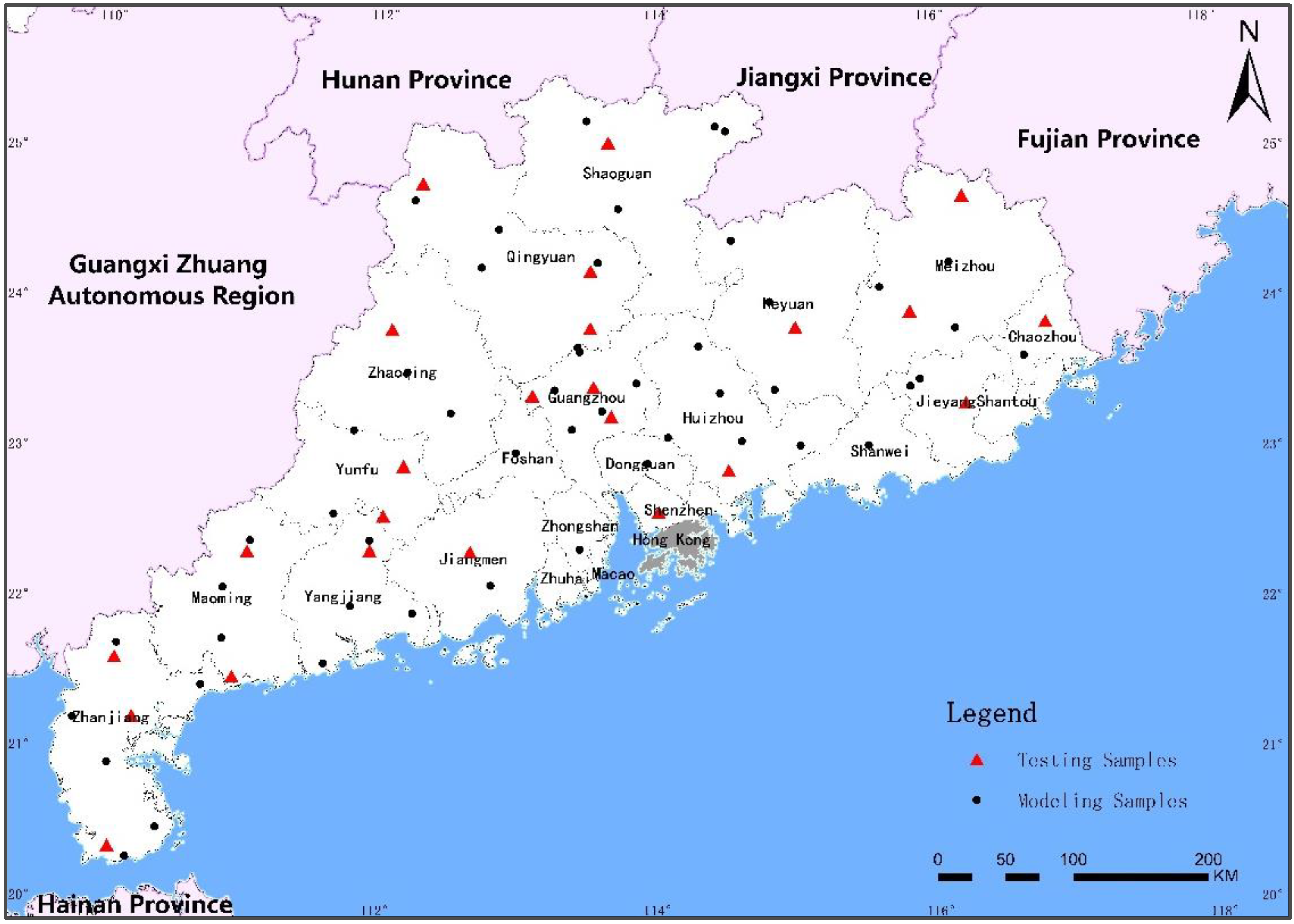
Guangdong Province in southern China is located at 20.13′–25.31′ N and 109.39′–117.19′ E. The study area overview is shown in Figure 1. The area of the province is 179,700 km2. The northern region is mostly hilly and has a relatively high elevation. The southern coastal area has relatively low altitude and the terrain is relatively flat. Guangdong Province has a subtropical monsoon climate, the average sunshine duration in the province is 1745.8 h, the annual average temperature is 22.3 °C, and the average annual precipitation is between 1300 and 2500 mm. It is one of the regions with the most abundant light, heat, and water resources in China. Since the reform and opening up, Guangdong Province has achieved rapid economic development and high levels of urbanization. It is a province with major economic development and urbanization in China. With the development of the economy, the level of industrialization is also continuously improving and, therefore, the area has become one of the provinces in China where soil heavy metal pollution is relatively serious.
2.2. Acquisition and Processing of Soil Data
A total of 75 soil samples were collected in Guangdong Province and were located using GPS positioning; the sampling was conducted at a depth of 0–20 cm and the samples weighed about 300 g. Field samples were collected at 50 km × 50 km scale of sampling grid, and the sample points in densely populated areas and possibly contaminated areas were mainly collected at 30 km × 30 km scale of sampling grid. The sample locations are shown in Figure 1. The soil samples were taken back to the laboratory and naturally dried and the gravel and the residues of animals and plants were removed. Each sample was divided into two parts after grinding and sieving to 0.2 mm for determining the soil heavy metal content and the soil spectral reflectance. For the determination of the soil mercury content, a sample amount of 0.2 g was digested with H2SO4-HNO3-KMnO4 and cold atomic absorption was used. The descriptive statistics of the mercury content of the 75 soil samples are shown in Table 1.
The maximum soil mercury content in the study area was 0.615 mg/kg, the minimum was 0.018 mg/kg, and the average was 0.139 mg/kg, which was 1.782 times the background value of Guangdong. The variation coefficient of the mercury content in the soil samples is 84.89%. Generally, the variation coefficient reflects the degree of dispersion and the ranges is between 10% and 100%. Therefore, the soil mercury content in the study area has moderate variability. In order to clarify the model establishment and verification, a comprehensive explanation of the pros and cons of each model is provided. In the subsequent data processing, the 75 samples are arranged in descending order of mercury content and every third sample (25 samples) is used as a test sample and the remaining 50 samples are used as modeling samples to ensure consistency between the modeling and the test samples and an even distribution, as shown in Figure 1.
2.3. Collection and Processing of Soil Spectral Data
The soil spectral reflectance was measured using an AvaField portable spectrometer manufactured by Avantes, Holland. The band range was 340.316–2511.179 nm, the spectral sampling interval was 0.6 nm, and the measurement light source was a 50-W halogen lamp; the light source was connected to the probe via an optical fiber and the field of view angle was 10°. The soil sample was placed in a sample dish with a diameter larger than 10 cm and a depth greater than 5 cm and the spectral data were collected by aligning the probe perpendicular to the soil sample. A standard whiteboard calibration was performed prior to each collection. Each soil sample was measured five times and 10 data points were automatically collected. The AvaReader software was used to eliminate the anomalous data and the mean value of the spectral reflectance was used as the reflectance value of the sample.
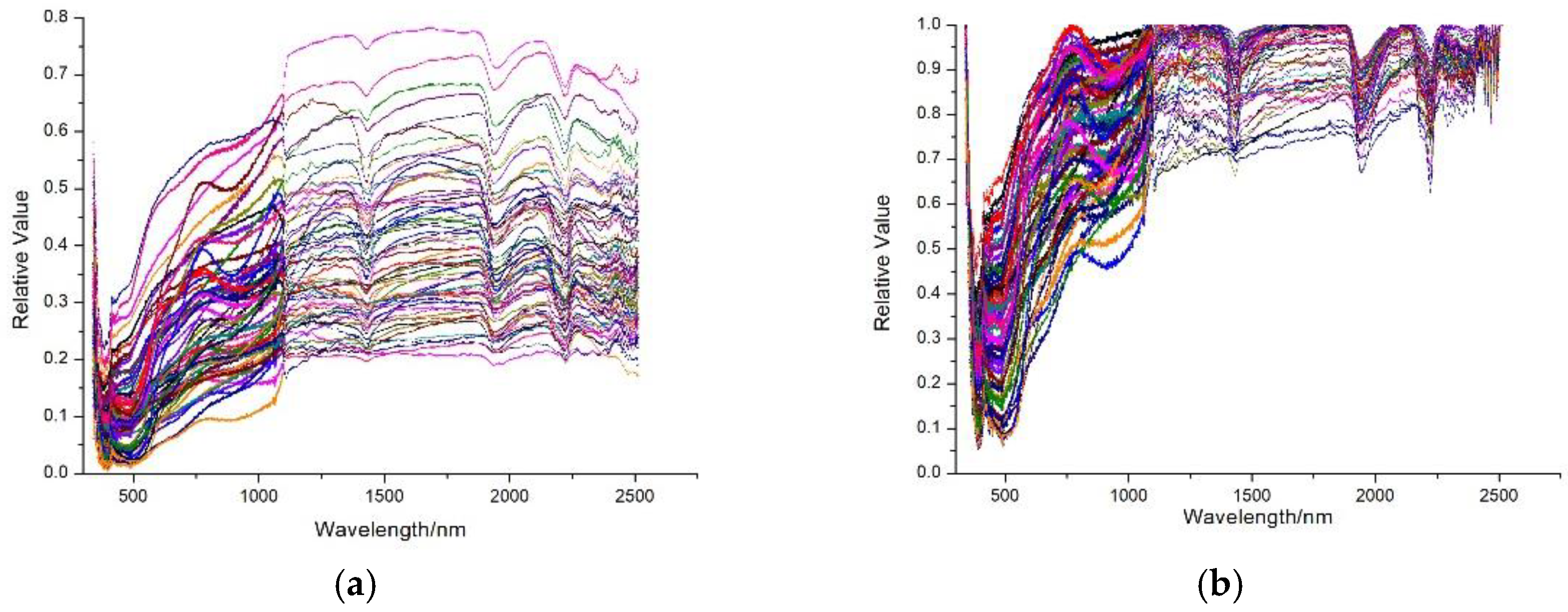
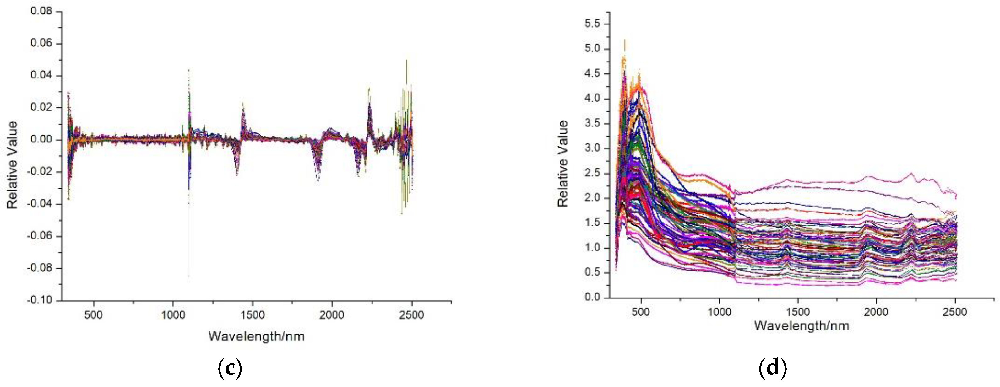
The spectral measurements are easily influenced by many factors such as the observation angle, illumination, and the surface roughness of the sample; these effects result in a relatively low signal-to-noise ratio (SNR) of the spectral data. Therefore, a transformation process needs to be performed. After the transformation, the original spectral data can be transformed to eliminate the background noise, enhance the difference, and highlight the absorption and reflection characteristics of the spectral curve. In this study, the Savitzky-Golay smoothing filter was used for smoothing and optimization of the spectral curve. The smoothed curve retains the information of the data, as shown in Figure 2a. Based on the smoothed spectral curves, continuum removal (CR), first-order differential (FD), and reciprocal logarithmic (RL) processing were performed separately. The results are shown in Figure 2b–d.
2.4. Modeling Method
2.4.1. Feature Band Selection
A relationship exists between the spectral reflectance and the soil mercury content. We used a correlation analysis and a significance level greater than p = 0.01 to determine the bands with high correlation coefficients; the variance inflation factor (VIF) was used to verify the autocorrelation between the bands. The larger the value of the VIF, the greater the collinearity is. The empirical evaluation showed that no multicollinearity existed at VIF values between 0 and 10; at VIF values between 10 and 100, there was high multicollinearity and at VIF values greater than 100, there was very high multicollinearity. In this study, Pearson’s correlation coefficient was used to describe the relationship between the soil spectral characteristics and the soil mercury content. The Pearson’s correlation coefficient reflects the degree of linear correlation between the two variables and is one of the most widely used relational measures. It is defined as the product of the covariance of two variables divided by the product of the standard deviation of the two variables [20]; Pearson’s correlation coefficient is expressed as shown in Equation (1):
where is the reflectance of the ith band, is the ith soil mercury content, is the average of the band reflectance, and is the average mercury content of the soil. The range of the coefficient is [−1, 1]. When the sign is positive, the two variables are positively correlated and vice versa. The greater the absolute value of the coefficient, the greater the linear correlation between the two variables is.
2.4.2. MLR Method for Determination of the Soil Mercury Content
The MLR method was first proposed by Francis Galton in the late 19th century and was used for model prediction in the early days. It is a classical statistical analysis method based on the least squares method and is used to establish a linear equation to explain the relationship between two or more independent variables and a dependent variable [8,21]. The general form of the model is shown in Equation (2):
where Y is the soil mercury content, is the reflectance of the jth feature band, is the jth regression coefficient, n is the number of feature bands, and ε is the random error. The matrix expression of the equation is shown in Equation (3):
where X is the full rank matrix and β is predicted by the least squares method. The estimated value is calculated by Equation (4):
Therefore, according to Equations (3) and (4), the predicted value of the soil mercury content is calculated by Equation (5):
2.4.3. BPNN Method for Determination of the Soil Mercury Content
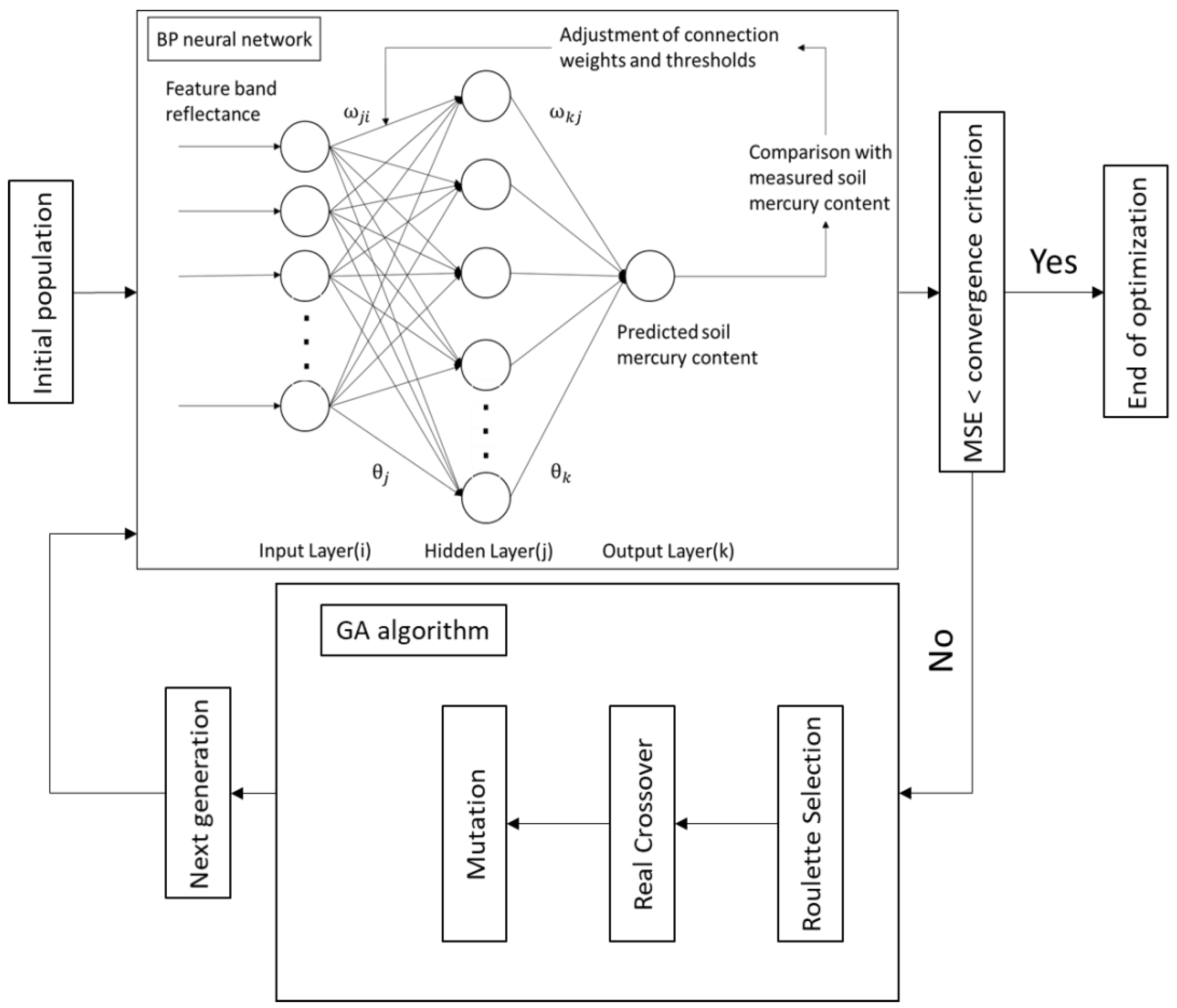
In this study, a BPNN is used to predict the soil mercury content. The structure of the BPNN is shown in Figure 3 and it can be called a “black box” model. The BPNN learns and is trained by a guided learning method that predicts the relationship between any nonlinear input variable and output variable. The learning process is composed of forward propagation of the input signal and BP of the error. The training process consists of continuously adjusting the connection weights until the output error reaches a required standard [22].
The input layer to the hidden layer is expressed as shown in Equation (6):
where is the input layer information, which in this case is the reflectance of the feature band; is the hidden layer information; represents the weight of the input layer to the hidden layer; and is the transfer function of the input layer to the hidden layer. This is generally a sigmoid function but in this study, the tansig function is used; is the threshold of the hidden layer.
The hidden layer to the output layer is expressed as shown in Equation (7):
where is the output layer information, which in this case is the predicted value of the soil mercury content; represents the weight of the hidden layer to the output layer; is the transfer function of the hidden layer to the output layer; the purelin function is selected in this study; is the threshold of the output layer.
If there is a large difference between the predicted value and the measured value, this discrepancy is transferred to the error propagation process. The BP process uses the Levenberg-Marquardt algorithm to correct the connection weights from the output layer to the input layer to reduce the mean squared error:
where o is the measured soil mercury content and N is the number of training samples.
2.4.4. GA-BPNN Method for Determination of the Soil Mercury Content
A GA is a stochastic global search and optimization method that mimics the biological evolution mechanism in nature. It is robust, does not easily fall into a local optimum, and can be used for parallel distributed processing [23]. Therefore, we combined the GA and BPNN by using the population search method to optimize the weights and thresholds of the NN; the structure of the GA-BPNN is shown in Figure 3.
We use a real-number coding method to transform the initial weights and thresholds in the BPNN into chromosomes in the GA. The code length is calculated using Equation (9):
where i is the number of input layer neuron nodes, which in this case is the number of feature bands; k is the number of output layer neuron nodes; k = 1 because the output layer consists only of the soil mercury content; j is the number of hidden layer neuron nodes. Then, a random population of chromosomes is generated. The BPNN is used to obtain the sum of the absolute value of the error between the predicted and measured values of the training data as the individual fitness value. The formula is shown in Equation (10):
where is the measured value of the mercury content in the kth soil sample; is the predicted value of the mercury content in the kth soil sample. The larger the fitness value, the larger the error is; therefore, the reciprocal of the fitness value should be used prior to the selection operation. Furthermore, individual evolutionary operations such as roulette selection, real crossover, and mutation are performed until the training target reaches the preset requirements or the number of iterations is reached. The optimal solution of the GA is used as the initial weight and the threshold of the BPNN, that is, ω and θ in Equations (6) and (7); subsequently, the BPNN is trained to obtain the optimal solution.
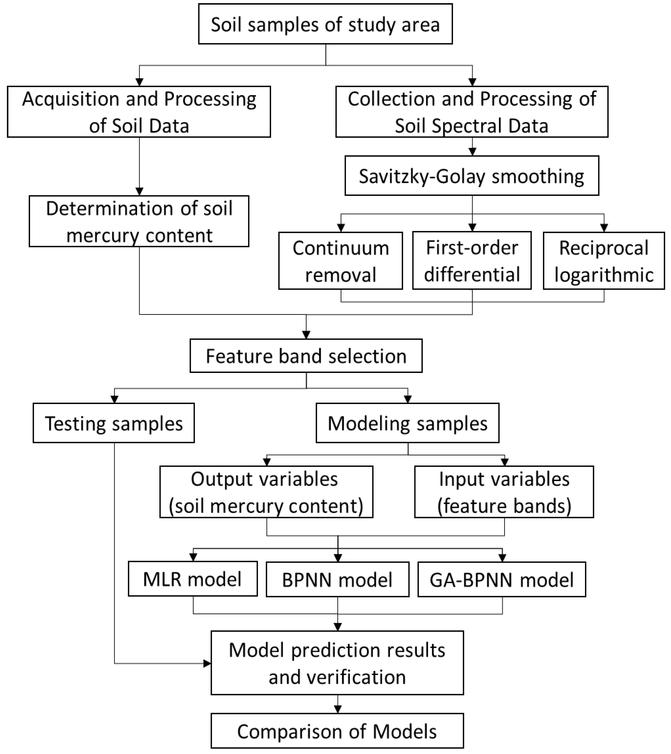
To effectively determine the optimal soil mercury content simulation method, we present a flow chart which is shown in Figure 4.
3. Results
3.1. Feature Band Selection Results
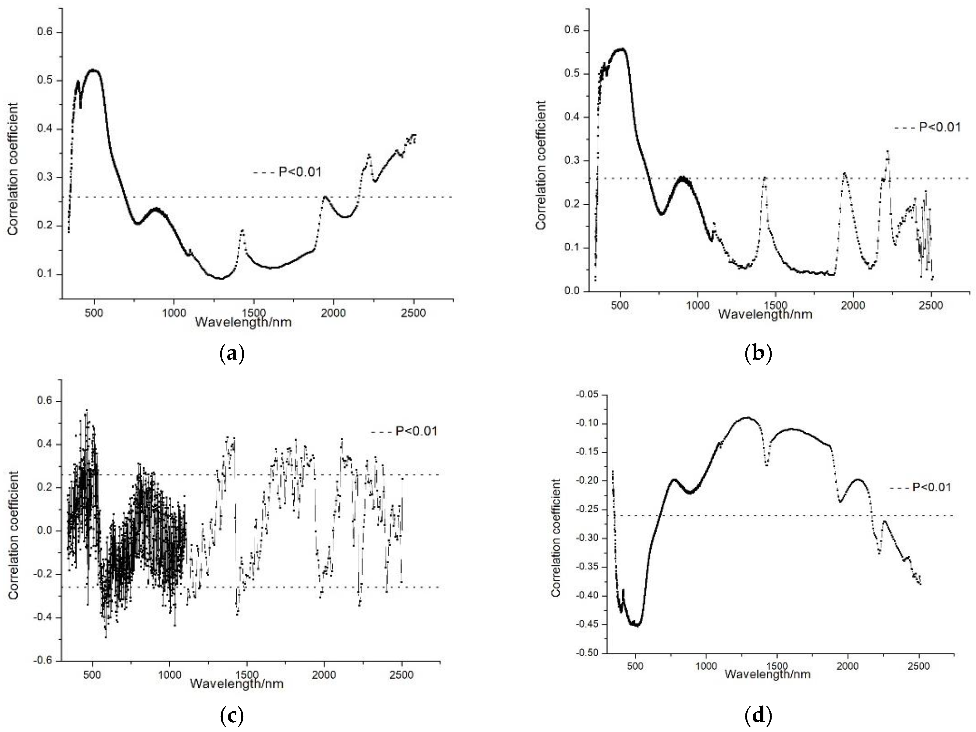
The Pearson’s correlation analysis was performed using the four spectral indices (i.e., the smoothed spectral reflectance, CR spectral reflectance, FD spectral reflectance, and RL spectral reflectance) and the soil mercury content; the result is shown in Figure 5.
It can be seen that the absolute value of the correlation coefficient between the spectral reflectance (the smoothed spectral reflectance is in the wavelength range of 350–695 nm and 2216–2228 nm, the CR spectral reflectance is in the range of 356–685 nm and 2200–2228 nm, and the RL spectral reflectance is in the range of 355–674 nm and 2171–2500 nm) and the soil mercury content was greater than 0.260 (significance level of p = 0.01), which means that the correlation is significant. The correlation coefficient between the FD spectral reflectance and the soil mercury content was considerably higher than the coefficients for the other three spectral indices and the number of bands with a correlation coefficient greater than 0.260 was higher; in addition, the absolute values of the correlation coefficients were significantly higher. It was found that the highest positive correlations of the FD spectral reflectance occurred at 465.351 nm, 799.18 nm, 1373.48 nm, and 2114.978 nm and the lowest negative correlations occurred at 587.705 nm, 1035.788 nm, and 1975.4 nm; the absolute values of these correlation coefficients are all greater than 0.300. Therefore, we selected the bands where the correlation coefficients were highest or lowest and had no collinearity to predict the soil mercury content. A total of 13 bands were selected as the feature bands, as shown in Table 2.
3.2. Modeling Results
3.2.1. MLR Model Prediction Results of Soil Mercury Content
In this study, 13 feature bands were used as independent variables and the corresponding soil mercury content was used as the dependent variable to perform a regression analysis using Equation (2). The MLR model is shown in Equation (11):
The predicted value is obtained and is compared with the measured value. The result is shown in Figure 6; the X-coordinates are the measured values, and the Y-coordinates are the predicted values.
In this study, three indicators are selected to test the accuracy of the model; these are the coefficient of determination (R2), root mean squared error (RMSE), and mean absolute error (MAE), as shown in Equations (12)–(14). The range of R2 is [0, 1]; the larger the R2 value, the stronger the linear relationship between the measured value and the predicted value is and the more stable the model is. The smaller the RMSE and MAE, the better the model predictability is.
where y is the measured value of the soil mercury content; is the predicted value of the soil mercury content; is the measured mean value of the soil mercury content; n is the number of samples.
The predicted value of the MLR model is quite different from the measured value. There are many points that exhibit large differences and a trend is apparent. The points deviate from the 1:1 line to varying degrees. The modeling is 0.665, the RMSE is 0.076, and the MAE is 0.059; the testing is 0.665, the RMSE is 0.087, and the MAE is 0.063.
3.2.2. BPNN Model Prediction Results of Soil Mercury Content
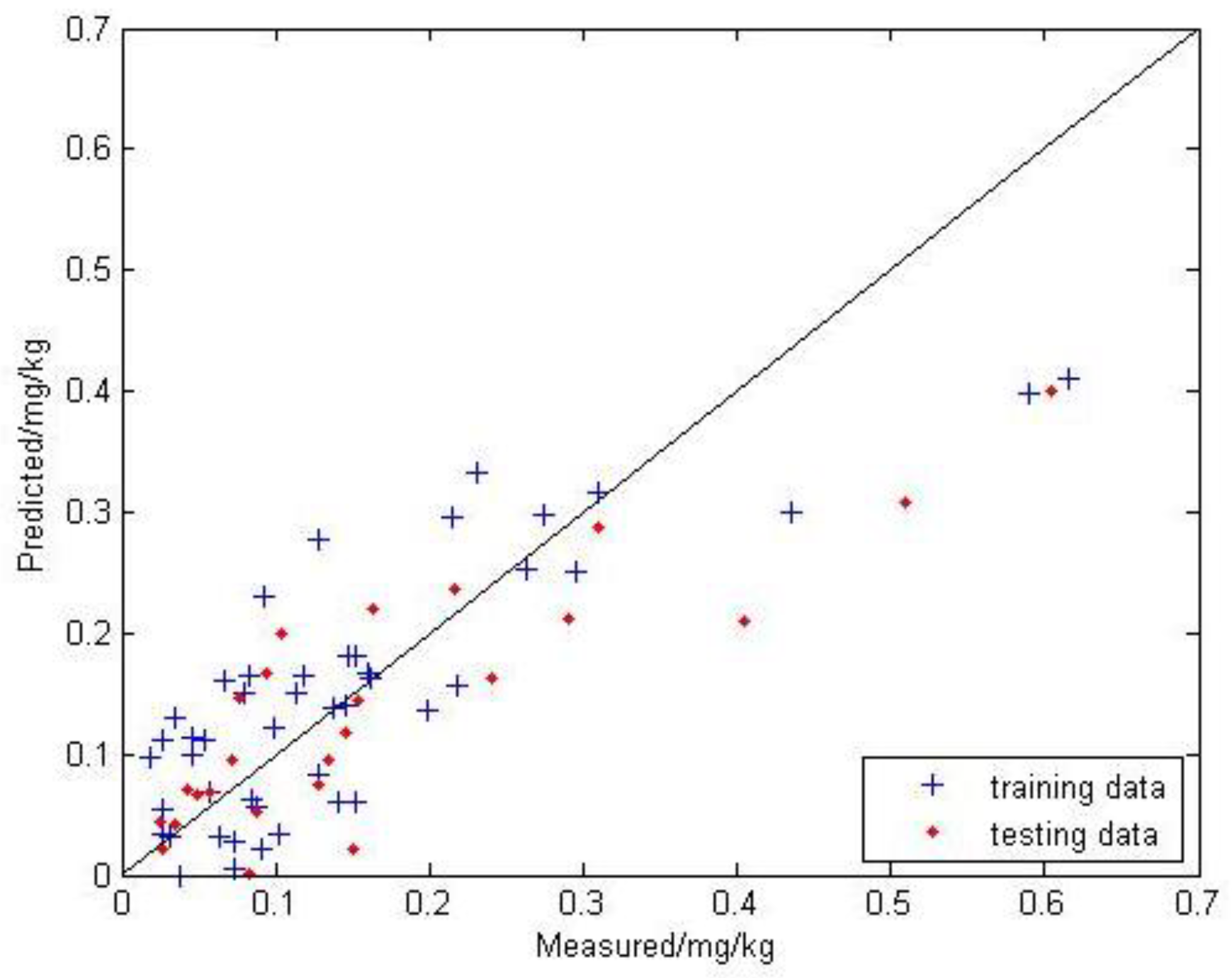
A three-layer BPNN with a single hidden layer was used to predict the soil mercury content in this study. An arbitrary nonlinear mapping is achieved by adjusting the number of neurons in the hidden layer. The input layer of the network was composed of the reflectance of the 13 feature bands and the output layer was the soil mercury content. Through several experiments, it was finally determined that the number of neurons in the hidden layer was 13, the learning rate was 0.1, the training frequency was 1000, and the expected error was 0.0001. The result is shown in Figure 7.
In the BPNN model, the points are located close to the 1:1 line but a few points exhibit slight deviations. The modeling is 0.797, the RMSE is 0.059, and the MAE is 0.032; the testing is 0.826, the RMSE is 0.063, and the MAE is 0.048.
3.2.3. GA-BPNN Model Prediction Results of Soil Mercury Content
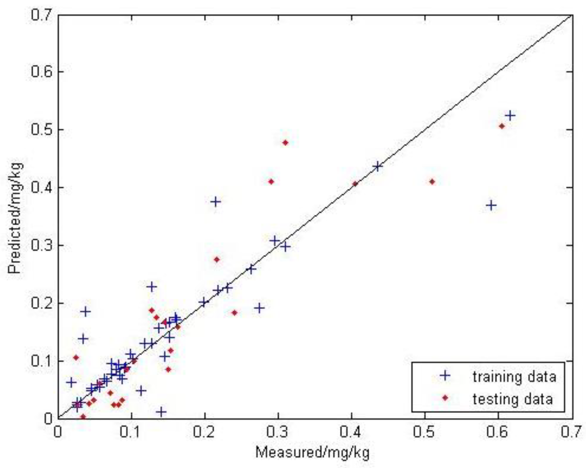
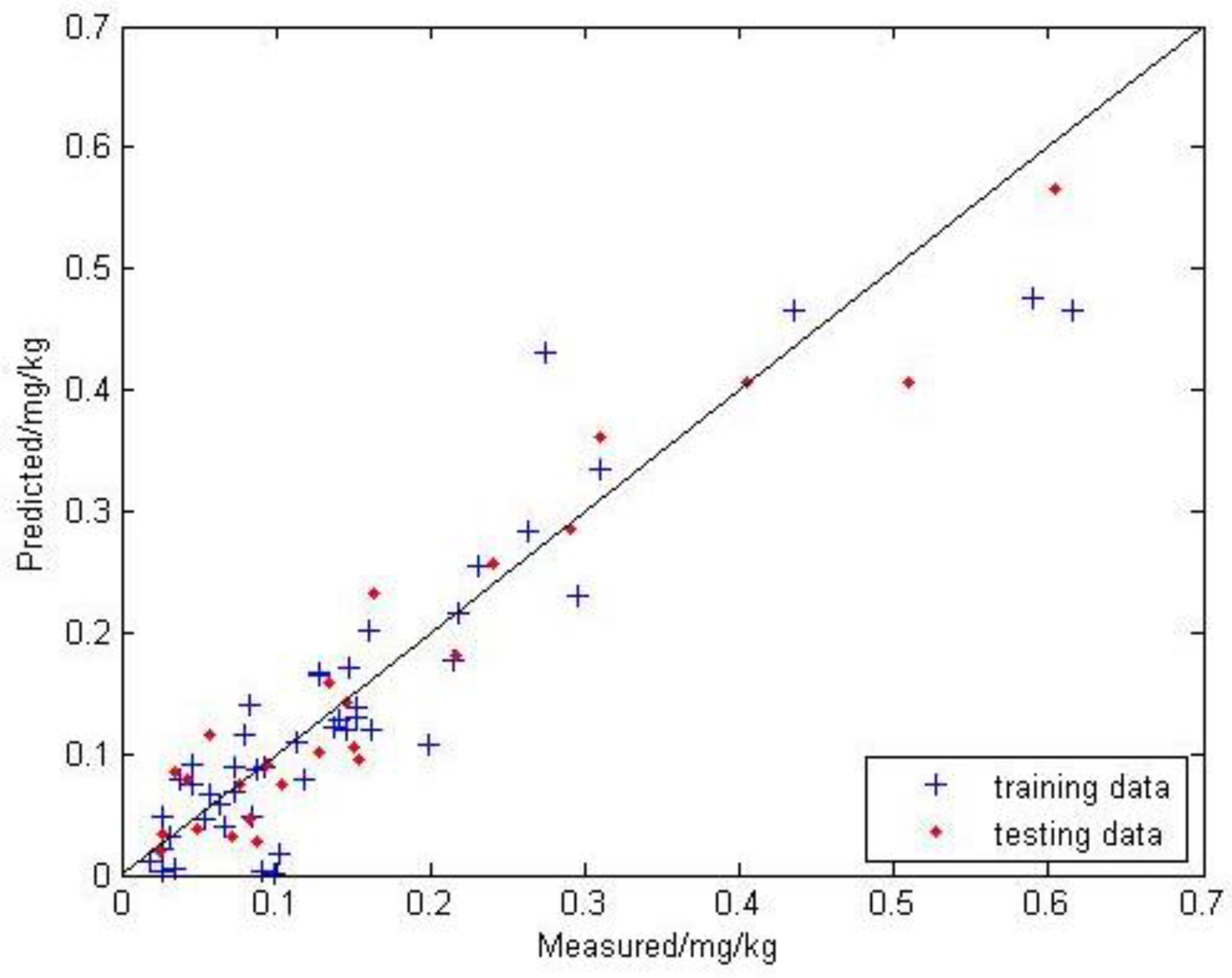
In order to compare the results of the GA optimization more accurately, the network structure and parameter configuration were the same as in the BPNN. The evolution algebra is set to 100 times, the population size is 64, the crossover probability is 0.4, and the mutation probability is 0.07. The result is shown in Figure 8.
In the GA-BPNN model, the points are located closest to the 1:1 line and the trend is more consistent with the 1:1 line. The modeling is 0.842, the RMSE is 0.052, and the MAE is 0.037; the testing is 0.923, the RMSE is 0.042, and the MAE is 0.033.
3.2.4. Comparison of Models
The model accuracy indicators are shown in Table 3. It is evident that the MLR model is inferior to the BPNN and GA-BPNN models both in modeling accuracy and testing accuracy. This shows that there is a clear non-linear relationship between the selected feature bands and the soil mercury content. For non-linear modeling, the GA-BPNN model performs better than the BPNN model, except that the modeling MAE of the GA-BPNN model is slightly inferior to that of the BPNN model.
Table 4 shows the predicted and measured soil mercury contents of the three models. It can be seen that the predicted range and mean values of the sample are close to the range and average of the measured values for the nonlinear model, further illustrating the apparent nonlinear relationship between the selected feature bands and the soil mercury content. In nonlinear modeling, although the average predicted value of the test samples is close to the average measured value for the BPNN model, the range of the predicted values of the test samples is close to the measured value range for the GA-BPNN model and the MAE and MRE of GA-BPNN model are lowest among the models. In conclusion, the GA-BPNN model is the optimal model for predicting the soil mercury content.
4. Discussion
In this study, we selected 13 spectral bands (, , , , , , , , , , , , and ) according to the biggest or smallest of the correlation coefficient and selected the bands with no collinearity. The research results are in agreement with the results of previous studies [15,24], which implies that the selected bands were reliable.
Hyperspectral prediction models of soil mercury content were established using MLR, BPNN, and GA-BPNN. After analyzing and comparing the results of the three methods, it was found that the GA-BPNN model was the best model for predicting the mercury content in soil; the was 0.842 and the RMSE was 0.052. The superiority of the GA-BPNN model was attributed to the optimization of the BPNN initial input parameters (thresholds and weights) by the GA algorithm; this approach does not have the problem of low accuracy common in MLR methods.
The data in Table 4 indicate that larger errors were observed for the soil samples with high soil mercury content because few samples with high soil mercury content were used to train the MLR, BPNN and GA-BPNN models. Thus, in order to improve the prediction accuracy of the soil mercury content, more soil samples with high mercury content have to be collected to develop soil mercury models in the future.
Otherwise, the study was limited to individual sample points. In order to determine the soil mercury content at the regional scale, hyperspectral images should be combined with the models.
5. Conclusions
In this study, soil samples from Guangdong Province were used to determine the soil mercury content by mathematically transforming the soil spectral reflectance data using the Savitzky-Golay smoothing, CR, FD, and RL processing. A Pearson’s correlation analysis was performed on the transformed spectral data and the soil mercury content; a total of 13 bands (, , , , , , , , , , , , and ) with high correlation coefficients, a significance of correlation, and no collinearity were selected. MLR, BPNN, and GA-BPNN were used to establish hyperspectral prediction models of soil mercury content. After analyzing and comparing the results of the three methods, the GA-BPNN model was the optimum model for predicting the soil mercury content and the modeling was 0.842, the RMSE was 0.052, and the MAE was 0.037; the testing was 0.923, the RMSE was 0.042, and the MAE was 0.033. The results show that the GA-BPNN model is effective and accurate for predicting soil mercury content.
Author Contributions
The author contributions as follows: “Conceptualization, Y.-M.H., L.W. and Z.-H.L.; Methodology, L.Z., Y.-M.H., L.W. and Z.-H.L.; Validation, W.Z., Y.-C.P. and Z.S.; Formal Analysis, L.Z.; Investigation, L.Z.; Resources, Y.-M.H. and Z.-H.L.; Data Curation, L.Z. and W.Z.; Writing-Original Draft Preparation, L.Z.; Writing-Review & Editing, Z.-H.L. and G.-X.W.; Supervision, W.Z.; Project Administration, Z.-H.L.; Funding Acquisition, Y.-M.H.”.
Funding
This research was funded by [the National Key Research and Development Program of China (“Source Identification and Contamination Characteristics of Heavy Metals in Agricultural Land and Products”)], grant number [2016YFD0800301]; [the Guangdong Provincial Science and Technology Project of China], grant number [2017A050501031]; [the Guangzhou Science and Technology Project, China], [201804020034].
Acknowledgments
We really appreciate the technical assistance of Ying-Qiang Song, and writing assistance of Yi-Ping Peng.
Conflicts of Interest
The authors declare no conflict of interest.
References
- Pirrone, N.; Cinnirella, S.; Feng, X.; Finkelman, R.B.; Friedli, H.R.; Leaner, J.; Mason, R.; Mukherjee, A.B.; Stracher, G.B.; Streets, D.G.; et al. Global mercury emissions to the atmosphere from anthropogenic and natural sources. Atmos. Chem. Phys. Discuss. 2010, 10, 5951–5964. [Google Scholar] [CrossRef] [Green Version]
- Yin, R.S.; Feng, X.B.; Shi, W.F. Application of the stable-isotope system to the study of sources and fate of Hg in the environment: A review. Appl. Geochem. 2010, 25, 1467–1477. [Google Scholar] [CrossRef]
- Sun, W.; Zhang, X. Estimating soil zinc concentrations using reflectance spectroscopy. Int. J. Appl. Earth Obs. Geoinf. 2017, 58, 126–133. [Google Scholar] [CrossRef]
- Leenaers, H.; Okx, J.P.; Burrough, P.A. Employing elevation data for efficient mapping of soil pollution on floodplains. Soil Use Manag. 2010, 6, 105–114. [Google Scholar] [CrossRef]
- Choe, E.; van der Meer, F.; van Ruitenbeek, F.; van der Werff, H.; de Smeth, B.; Kim, K.W. Mapping of heavy metal pollution in stream sediments using combined geochemistry, field spectroscopy, and hyperspectral remote sensing: A case study of the Rodalquilar mining area, SE Spain. Remote Sens. Environ. 2008, 112, 3222–3233. [Google Scholar] [CrossRef]
- Liu, M.; Liu, X.; Ding, W.; Wu, L. Monitoring stress levels on rice with heavy metal pollution from hyperspectral reflectance data using wavelet-fractal analysis. Int. J. Appl. Earth Obs. Geoinf. 2011, 13, 246–255. [Google Scholar] [CrossRef]
- Idowu, O.J.; van Es, H.M.; Abawi, G.S.; Wolfe, D.W.; Ball, J.I.; Gugino, B.K.; Moebius, B.N.; Schindelbeck, R.R.; Bilgili, A.V. Farmer-oriented assessment of soil quality using field, laboratory, and VNIR spectroscopy methods. Plant Soil 2008, 307, 243–253. [Google Scholar] [CrossRef]
- Dong, J.; Dai, W.; Xu, J.; Li, S. Spectral Estimation Model Construction of Heavy Metals in Mining Reclamation Areas. Int. J. Environ. Res. Public Health 2016, 13, 640. [Google Scholar] [CrossRef] [PubMed]
- Wu, Y.Z.; Chen, J.; Ji, J.F.; Tian, Q.J.; Wu, X.M. Feasibility of reflectance spectroscopy for the assessment of soil mercury contamination. Environ. Sci. Technol. 2005, 39, 873–878. [Google Scholar] [CrossRef] [PubMed]
- Zhang, N.; Liu, G.; Song, H. Using hyperspectral image data to estimate soil mercury with stepwise multiple regression. In Proceedings of the Eighth International Conference on Digital Image Processing, Chengdu, China, 29 August 2016. 100333Q. [Google Scholar]
- Choe, E.; Kim, K.W.; Bang, S.; Yoon, I.H.; Lee, K.Y. Qualitative analysis and mapping of heavy metals in an abandoned Au–Ag mine area using NIR spectroscopy. Environ. Geol. 2009, 58, 477–482. [Google Scholar] [CrossRef]
- Chang, C.W.; Laird, D.A.; Mausbach, M.J.; Hurburgh, C.R. Near-Infrared Reflectance Spectroscopy–Principal Components Regression Analyses of Soil Properties. Soil Sci. Soc. Am. J. 2001, 65, 480–490. [Google Scholar] [CrossRef]
- Xia, F.; Peng, J.; Wang, Q.L.; Zhou, L.Q.; Shi, Z. Prediction of heavy metal content in soil of cultivated land: Hyperspectral technology at provincial scale. J. Infrared Millim. Waves 2015, 34, 593–598, 605. [Google Scholar]
- Rathod, P.H.; Müller, I.; Van der Meer, F.D.; de Smeth, B. Analysis of visible and near infrared spectral reflectance for assessing metals in soil. Environ. Monit. Assess. 2015, 188, 558. [Google Scholar] [CrossRef] [PubMed]
- Wu, Y.; Chen, J.; Wu, X.; Tian, Q.; Ji, J.; Qin, Z. Possibilities of reflectance spectroscopy for the assessment of contaminant elements in suburban soils. Appl. Geochem. 2005, 20, 1051–1059. [Google Scholar] [CrossRef]
- Tan, K.; Ye, Y.; Cao, Q.; Du, P.; Dong, J. Estimation of Arsenic Contamination in Reclaimed Agricultural Soils Using Reflectance Spectroscopy and ANFIS Model. IEEE J. Sel. Top. Appl. Earth Obs. Remote Sens. 2014, 7, 2540–2546. [Google Scholar] [CrossRef]
- Dou, Y.; Qu, N.; Wang, B.; Chi, Y.Z.; Ren, Y.L. Simultaneous determination of two active components in compound aspirin tablets using principal component artificial neural networks (PC-ANNs) on NIR spectroscopy. Eur. J. Pharm. Sci. 2007, 32, 193–199. [Google Scholar] [CrossRef] [PubMed]
- Ma, W.-B.; Tan, K.; Li, H.-D.; Yan, Q.W. Hyperspectral Inversion of Heavy Metals in Soil of a Mining Area Using Extreme Learning Machine. J. Ecol. Rural Environ. 2016, 32, 213–218. [Google Scholar]
- Balabin, R.M.; Lomakina, E.I. Support vector machine regression (SVR/LS-SVM)—An alternative to neural networks (Ann) for analytical chemistry? Comparison of nonlinear methods on near infrared (NIR) spectroscopy data. Analyst 2011, 136, 1703–1712. [Google Scholar] [CrossRef] [PubMed]
- Zhou, H.; Deng, Z.; Xia, Y.; Fu, M. A new sampling method in particle filter based on Pearson correlation coefficient. Neurocomputing 2016, 216, 208–215. [Google Scholar] [CrossRef]
- He, F.; Zhang, L. Prediction model of end-point phosphorus content in BOF steelmaking process based on PCA and BP neural network. J. Process Control 2018, 66, 51–58. [Google Scholar] [CrossRef]
- Haque, M.E.; Sudhakar, K.V. ANN back-propagation prediction model for fracture toughness in micro alloy steel. Int. J. Fatigue 2002, 24, 1003–1010. [Google Scholar] [CrossRef]
- Hoseinian, F.S.; Rezai, B.; Kowsari, E. The nickel ion removal prediction model from aqueous solutions using a hybrid neural genetic algorithm. J. Environ. Manag. 2017, 204, 311–317. [Google Scholar] [CrossRef] [PubMed]
- Liu, J.; Dong, Z.; Sun, Z.; Ma, H.; Shi, L. Study on Hyperspectral Characteristics and Estimation Model of Soil Mercury Content. In Materials Science and Engineering Conference Series; IOP Publishing Ltd.: Bristol, UK, 2017. [Google Scholar]
Figure 1.
Study area and the distribution of the soil sampling points.

Figure 2.
The spectral reflectance curves of the soil samples. (a) Smoothed spectral curves; (b) continuum removal spectral curves; (c) first-order differential spectral curves; (d) reciprocal logarithmic spectral curves.
Figure 2.
The spectral reflectance curves of the soil samples. (a) Smoothed spectral curves; (b) continuum removal spectral curves; (c) first-order differential spectral curves; (d) reciprocal logarithmic spectral curves.


Figure 3.
The structure of the GA-BPNN.

Figure 4.
Flow chart for determining the optimal soil mercury content simulation method.

Figure 5.
Correlation coefficients between soil spectral indices and soil mercury content. (a) The soil mercury content and the smoothed spectral reflectance; (b) the soil mercury content and the CR spectral reflectance; (c) the soil mercury content and the FD spectral reflectance; (d) the soil mercury content and the RL spectral reflectance.

Figure 6.
Measured and MLR predicted values of the soil mercury content.

Figure 7.
Measured and BPNN predicted values of the soil mercury content.

Figure 8.
Measured and GA-BPNN predicted values of the soil mercury content.


Table 1.
Descriptive statistics of the soil mercury content.
| No. | Mean/(mg/kg) | Max/(mg/kg) | Min/(mg/kg) | Std. | Coefficient Variation/% | Background Value/(mg/kg) | Ratio |
|---|---|---|---|---|---|---|---|
| 75 | 0.139 | 0.615 | 0.018 | 0.118 | 84.89 | 0.078 | 1.782 |
Table 2.
The feature bands and the correlation coefficients.
| Feature Bands | Correlation Coefficients |
|---|---|
| , | 0.521, 0.346 |
| , | 0.556, 0.323 |
| , , , , , , | 0.558, −0.492, 0.313, −0.438, 0.433, −0.307, 0.426 |
| , | −0.453, −0.326 |
Table 3.
The accuracy indicators of the three models.
| Model | Modeling | Testing | ||||
|---|---|---|---|---|---|---|
| RMSE | MAE | RMSE | MAE | |||
| MLR | 0.665 | 0.076 | 0.059 | 0.665 | 0.087 | 0.063 |
| BPNN | 0.797 | 0.059 | 0.032 | 0.826 | 0.063 | 0.047 |
| GA-BPNN | 0.842 | 0.052 | 0.037 | 0.923 | 0.042 | 0.033 |
Table 4.
Predicted and measured values of soil mercury content for the tested models.
| No. | Predicted Value/(mg/kg) | Measured Value/(mg/kg) | Absolute Error | Relative Error | ||||||
|---|---|---|---|---|---|---|---|---|---|---|
| MLR | BPNN | GA-BPNN | MLR | BPNN | GA-BPNN | MLR | BPNN | GA-BPNN | ||
| 1 | 0.400 | 0.507 | 0.565 | 0.605 | 0.205 | 0.098 | 0.04 | 0.339 | 0.162 | 0.066 |
| 2 | 0.307 | 0.410 | 0.405 | 0.509 | 0.202 | 0.099 | 0.104 | 0.397 | 0.194 | 0.204 |
| 3 | 0.210 | 0.407 | 0.405 | 0.405 | 0.195 | 0.002 | 0 | 0.481 | 0.005 | 0.000 |
| 4 | 0.287 | 0.477 | 0.361 | 0.310 | 0.023 | 0.167 | 0.051 | 0.074 | 0.539 | 0.165 |
| 5 | 0.211 | 0.411 | 0.286 | 0.291 | 0.08 | 0.12 | 0.005 | 0.275 | 0.412 | 0.017 |
| 6 | 0.162 | 0.183 | 0.257 | 0.240 | 0.078 | 0.057 | 0.017 | 0.325 | 0.238 | 0.071 |
| 7 | 0.237 | 0.275 | 0.181 | 0.217 | 0.02 | 0.058 | 0.036 | 0.092 | 0.267 | 0.166 |
| 8 | 0.219 | 0.159 | 0.232 | 0.163 | 0.056 | 0.004 | 0.069 | 0.344 | 0.025 | 0.423 |
| 9 | 0.144 | 0.118 | 0.095 | 0.153 | 0.009 | 0.035 | 0.058 | 0.059 | 0.229 | 0.379 |
| 10 | 0.022 | 0.085 | 0.106 | 0.151 | 0.129 | 0.066 | 0.045 | 0.854 | 0.437 | 0.298 |
| 11 | 0.119 | 0.167 | 0.141 | 0.145 | 0.026 | 0.022 | 0.004 | 0.179 | 0.152 | 0.028 |
| 12 | 0.095 | 0.174 | 0.158 | 0.134 | 0.039 | 0.04 | 0.024 | 0.291 | 0.299 | 0.179 |
| 13 | 0.075 | 0.188 | 0.100 | 0.128 | 0.053 | 0.06 | 0.028 | 0.414 | 0.469 | 0.219 |
| 14 | 0.199 | 0.100 | 0.075 | 0.105 | 0.094 | 0.005 | 0.03 | 0.895 | 0.048 | 0.286 |
| 15 | 0.166 | 0.085 | 0.091 | 0.095 | 0.071 | 0.01 | 0.004 | 0.747 | 0.105 | 0.042 |
| 16 | 0.053 | 0.032 | 0.027 | 0.088 | 0.035 | 0.056 | 0.061 | 0.398 | 0.636 | 0.693 |
| 17 | 0.002 | 0.023 | 0.046 | 0.083 | 0.081 | 0.06 | 0.037 | 0.976 | 0.723 | 0.446 |
| 18 | 0.147 | 0.024 | 0.075 | 0.076 | 0.071 | 0.052 | 0.001 | 0.934 | 0.684 | 0.013 |
| 19 | 0.094 | 0.044 | 0.032 | 0.072 | 0.022 | 0.028 | 0.04 | 0.306 | 0.389 | 0.556 |
| 20 | 0.068 | 0.060 | 0.115 | 0.058 | 0.01 | 0.002 | 0.057 | 0.172 | 0.034 | 0.983 |
| 21 | 0.067 | 0.032 | 0.037 | 0.049 | 0.018 | 0.017 | 0.012 | 0.367 | 0.347 | 0.245 |
| 22 | 0.070 | 0.026 | 0.080 | 0.042 | 0.028 | 0.016 | 0.038 | 0.667 | 0.381 | 0.905 |
| 23 | 0.043 | 0.003 | 0.085 | 0.034 | 0.009 | 0.031 | 0.051 | 0.265 | 0.912 | 1.500 |
| 24 | 0.021 | 0.024 | 0.035 | 0.027 | 0.006 | 0.003 | 0.008 | 0.222 | 0.111 | 0.296 |
| 25 | 0.044 | 0.105 | 0.020 | 0.026 | 0.018 | 0.079 | 0.006 | 0.692 | 3.038 | 0.231 |
| Mean | 0.138 | 0.165 | 0.160 | 0.168 | 0.063 | 0.047 | 0.033 | 0.431 | 0.433 | 0.336 |
| Std. | 0.101 | 0.158 | 0.144 | 0.152 | ||||||
| MLR: 0.665 BPNN: 0.826 GA-BPNN: 0.923 | ||||||||||
| RMSE | MLR: 0.087 BPNN: 0.063 GA-BPNN: 0.042 | |||||||||
© 2018 by the authors. Licensee MDPI, Basel, Switzerland. This article is an open access article distributed under the terms and conditions of the Creative Commons Attribution (CC BY) license (http://creativecommons.org/licenses/by/4.0/).
Share and Cite
MDPI and ACS Style
Zhao, L.; Hu, Y.-M.; Zhou, W.; Liu, Z.-H.; Pan, Y.-C.; Shi, Z.; Wang, L.; Wang, G.-X. Estimation Methods for Soil Mercury Content Using Hyperspectral Remote Sensing. Sustainability 2018, 10, 2474. https://doi.org/10.3390/su10072474
AMA Style
Zhao L, Hu Y-M, Zhou W, Liu Z-H, Pan Y-C, Shi Z, Wang L, Wang G-X. Estimation Methods for Soil Mercury Content Using Hyperspectral Remote Sensing. Sustainability. 2018; 10(7):2474. https://doi.org/10.3390/su10072474
Chicago/Turabian StyleZhao, Li, Yue-Ming Hu, Wu Zhou, Zhen-Hua Liu, Yu-Chun Pan, Zhou Shi, Lu Wang, and Guang-Xing Wang. 2018. "Estimation Methods for Soil Mercury Content Using Hyperspectral Remote Sensing" Sustainability 10, no. 7: 2474. https://doi.org/10.3390/su10072474
Note that from the first issue of 2016, this journal uses article numbers instead of page numbers. See further details here.