Exploring Urban Spatial Feature with Dasymetric Mapping Based on Mobile Phone Data and LUR-2SFCAe Method

Abstract

Dasymetric mapping of high-resolution population facilitates the exploration of urban spatial feature. While most relevant studies are still challenged by weak spatial heterogeneity of ancillary data and quality of traditional census data, usually outdated, costly and inaccurate, this paper focuses on mobile phone data, which can be real-time and precise, and also strengthens spatial heterogeneity by its massive mobile phone base stations. However, user population recorded by mobile phone base stations have no fixed spatial boundary, and base stations often disperse in extremely uneven spatial distribution, this study defines a distance-decay supply–demand relation between mobile phone user population of gridded base station and its surrounding land patches, and outlines a dasymetric mapping method integrating two-step floating catchment area method (2SFCAe) and land use regression (LUR). The results indicate that LUR-2SFCAe method shows a high fitness of regression, provides population mapping at a finer scale and helps identify urban centrality and employment subcenters with detailed worktime and non-worktime populations. The work involving studies of dasymetric mapping based on LUR-2SFCAe method and mobile phone data proves to be encouraging, sheds light on the relationship between mobile phone users and nearby land use, brings about an integrated exploration of 2SFCAe in LUR with distance-decay effect and enhances spatial heterogeneity.

1. Background

Population mapping at a finer scale and higher resolution can play an important role in understanding urban spatial features, especially in the measurement of urban centrality [1,2] and identification of employment centers [3,4,5,6,7]. Therein, dasymetric mapping is considered as an effective method [8], which helps allocate population data to finer spatial units with ancillary data.

Progress has been made in studies on dasymetric mapping with the employment of various methods such as Weighted areal interpolation [9], Binary filtered areal weighting [10], Three-class and limiting variable [11,12], and Image texture [13]. However, two main challenges are found in previous literature on dasymetric mapping: (1) the ignorance of spatial heterogeneity inside every geographic unit, which may contain inhabitable and uninhabitable parts, or parts of different population density; and (2) the quality of source population data.

Most studies try to address spatial heterogeneity by fining geographic scale of ancillary data, ranging from Land use/land cover data (LULC) [14], soil sealing degree [15], nighttime lights, transportation network, elevation, and slope data extracted from satellite maps [16] to data with more classifications, such as cadastral information [17], tax parcel [18], buildings [19], Points of Interests (POIs) [20], and Volunteer Geographic Information (VGI) [21]. Although such methods have proven effective in improving the resolution of population mapping by enhancing spatial variance with increased amount of data categories, the accuracy of ancillary data still affects the results. Moreover, the census data used in most studies usually lag behind in timeliness, and are costly and inaccurate, which could jeopardize the result of population distribution as well.

Meanwhile, statistical linear regression has often been employed to examine the correlation result between population density and ancillary data to verify the result of dasymetric mapping [17,22]. Especially, in many related air pollution studies [23,24,25], dasymetric mapping for regression between land use and observed air quality data, known as land use regression (LUR), is used to identify the connection between variables and the associated land uses.

This article proposes that taking mobile phone data as a source of population distribution would highly improve the accuracy of dasymetric mapping. With the rapid development of Information and Communication Technology (ICT), mobile phone data have become an important source for studies of population distribution and behaviors of urban residents, such as identifying the commuting of residents [26,27]. Even so, few studies take mobile phone data as a solution to address those two problems, even though they provide relatively accurate user population and precise spatial location. Meanwhile, the massive amount of mobile phone base stations with corresponding data of user distribution all over the cities could offer information of spatial heterogeneity which has always been lacking in previous dasymetric mapping methods.

However, compared with the clear boundary of traditional census data, the spatial distribution of population data associated with mobile phone base stations has no stable boundary of service area. Generating Thiessen polygons with base stations could help define a border, but the highly uneven spatial distribution of base stations would bring more uncertainty into the mapping result.

The paper further presents an integrated methodology of LUR-2SFCAe with two-step floating catchment area (2SFCA) and LUR to address the problem. As the mobile phone user population recorded by base stations are related to surrounding land use distribution and influenced by the distance-decay pattern [28], the mathematical relation between user population and neighbor land uses is similar to the classic distance-decay demand–supply model in accessibility studies on public service, wherein the 2SFCA method has proven effective. That is to say, the population of nearby land is determined by not only user population of nearby base stations and various land uses, but also the distances to them.

This paper begins with an assumption that the original mobile phone data and land use data would result in unacceptable correlation due to an extremely uneven distribution of base stations which may locate in close proximity but with largely different user population. Therefore, a 1 km grid and its centroids are applied to statistically transform original data into gridded mobile phone data, which show relatively high correlation with land use data by the LUR-2SFCAe method. With a population mapping during work time and non-worktime, the spatial feature of Wuhan is explored.

The result of this study indicates that LUR-2SFCAe can be utilized in mapping population of high resolution with land use data and mobile phone data in forms of grids. It can also be used to identify spatial feature of population at different time. The methodology of LUR-2SFCAe in the present article is also applicable to related LUR studies.

2. Data Preparation

2.1. Study Area: Wuhan, China

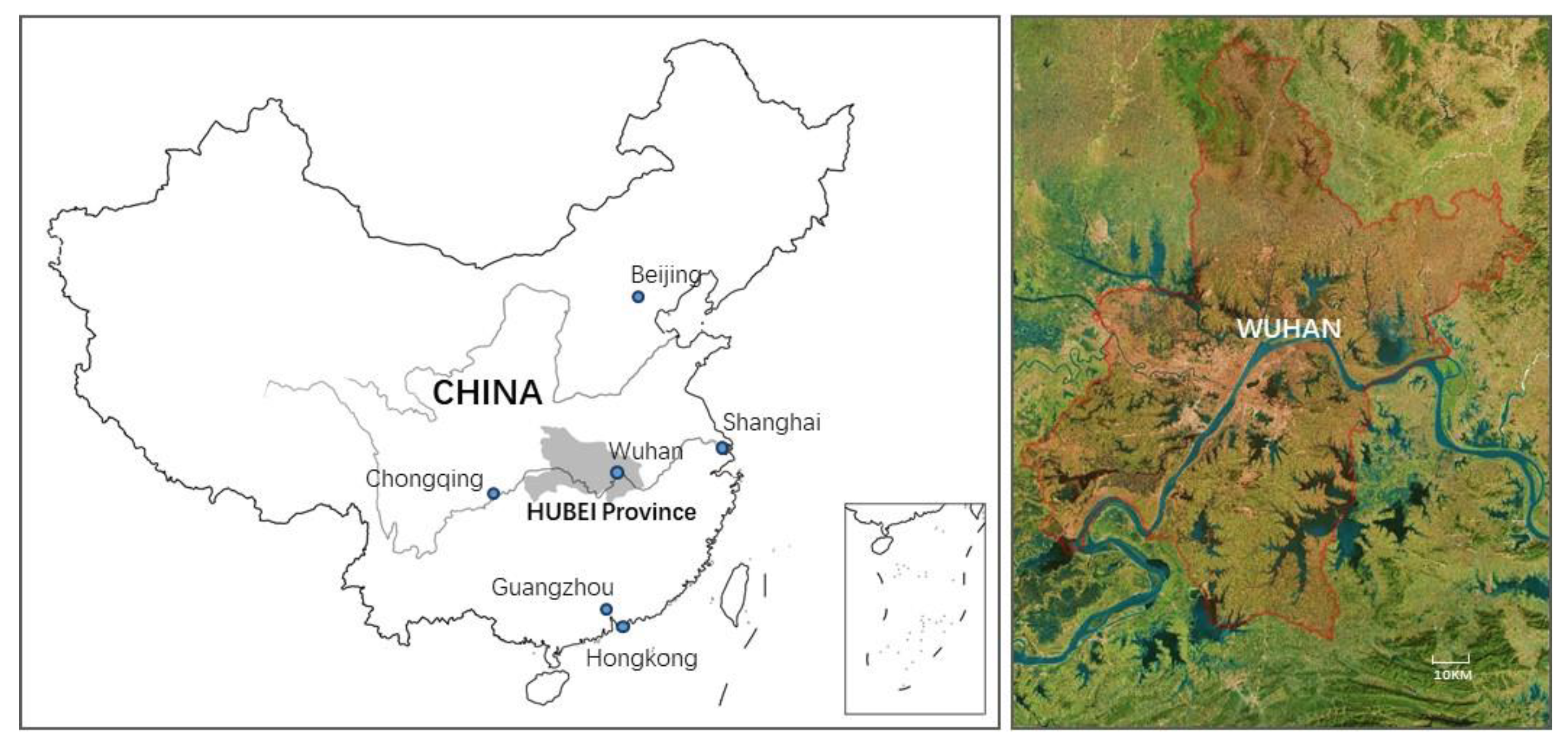
The case study area is Wuhan city, located in central China (Figure 1). As the capital of Hubei Province and one of the nine National Central Cities of China, Wuhan is the most populous city in Central China. The city boasts abundant mountain and water resources and is divided into “Three Towns” as Wuchang, Hankow, and Hanyang by the Yangtze River and Han River. The complicated geographic condition demands dasymetric mapping rather than simple interpolating tools such as Kriging, Kernel density or Voronoi polygons for population mapping.

2.2. Data and Preprocessing

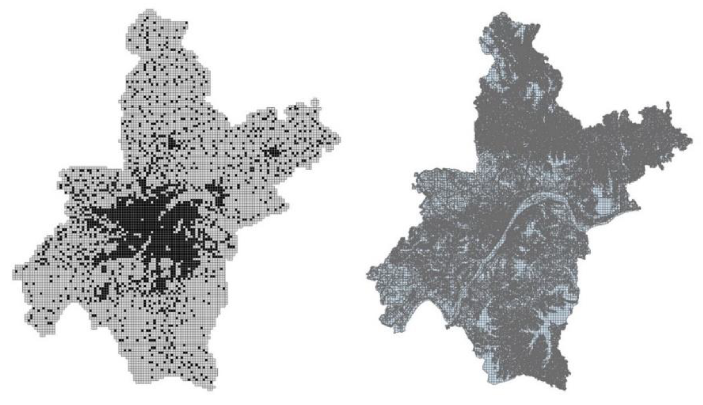
The present study utilizes two kinds of data in Wuhan metropolitan area: mobile phone data as the source population and existing land use as ancillary data; both were overlaid on the 1 km grids (Figure 2). The gridded data not only reflect the output resolution of population mapping but also improve the efficiency of model computing. Most importantly, the gridded mobile phone data can reduce the negative influence of uneven spatial distribution of original base stations in regression.

Land use data for 2013, provided by Wuhan Planning Bureau, were sorted in codes as A (Administration and public services), B (Commercial and business facilities), R (Residential), MW (Industrial, logistics and warehouse), S (Road, street and transportation), U (Municipal utilities), G (Green space and square) in urban built area, H (Development land, including town and country land as H1, regional infrastructure as H2, etc.) and E (Non-development land, including water as E1, farmland as E2, etc.) in the regional background.

After the grid was applied, each gridded land parcel and its centroid were assigned with the various types land uses.

Data of phone call records used in the present study were provided by a partner telecommunication operator whose market share is about 60%, verified for representing whole population distribution proportionally in Wuhan [29]. Mobile phone data of 7,300,000 users in November 2015 in Wuhan City were used in the study. As most urban studies of mobile phone data have discussed, the sample data can represent population distribution on a global scale, while users of other service providers and multiple data for the same user area have not been considered in the macro scope of whole city. Data were pre-processed, eliminating all privacy-related information. The basic format is a multi-field table tagged with the user ID. Data from the busiest base stations during one month were categorized into three time periods: work-time (from 7:00 a.m. to 7:00 p.m., Monday to Friday), and on-worktime (7:00 p.m. to 7:00 a.m., Monday to Friday; Saturdays and Sundays), and all-time.

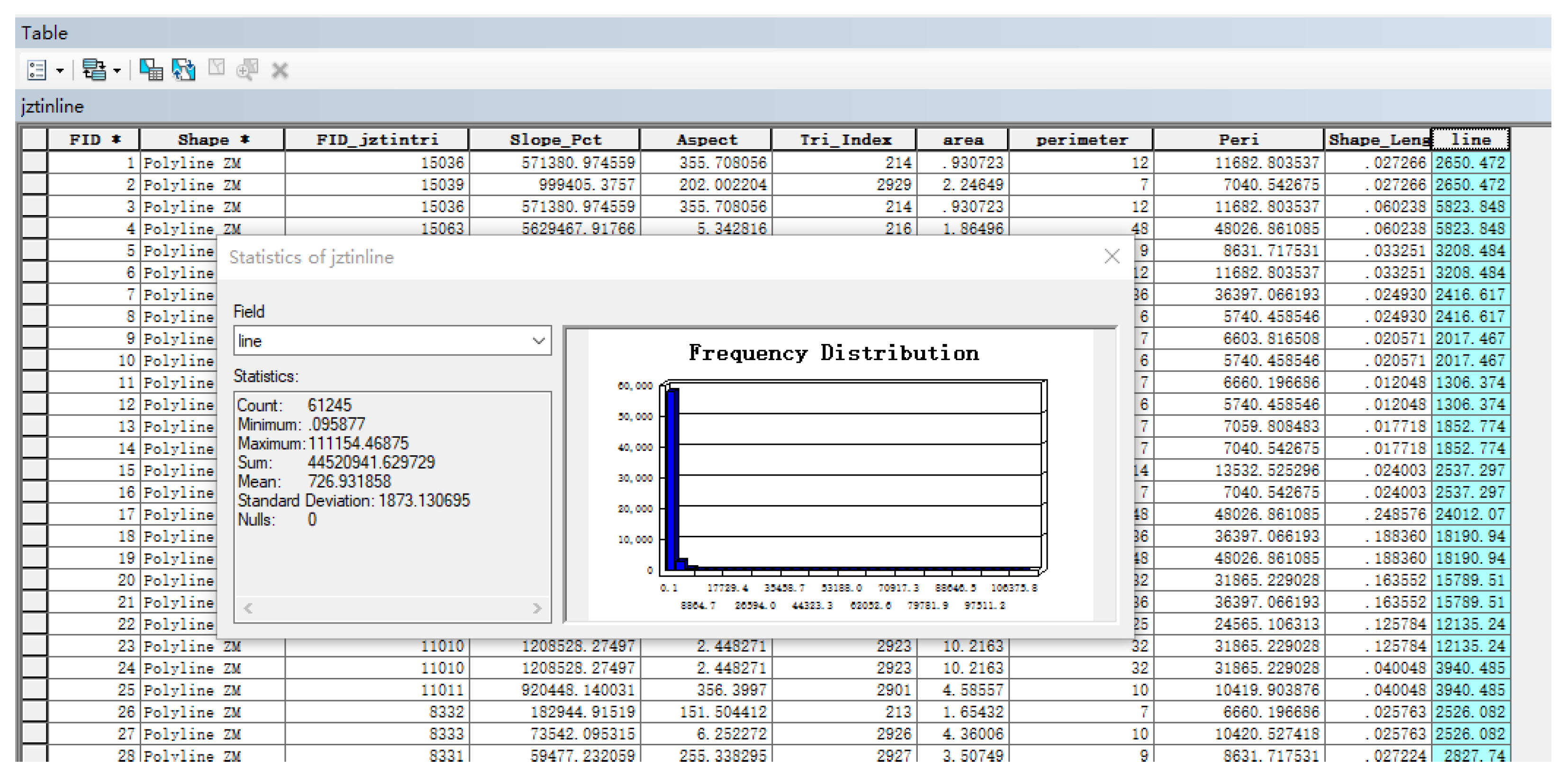
The distance based on the length statistics of TIN of all base stations in ArcGIS (Figure 3) shows that the minimum distance is 0.095877 m, the average value is 726.931858 m, and the standard deviation is 1873.130695 m. The spatial distribution of base station is extremely uneven, wherein base stations located nearby but with different user population would create significant error for land use regression.

Therefore, a 1 km grid was also applied to allocate the mobile phone data, generating a simulative grid of mobile phone data with centroids, evenly distributed spatially. The original 33,587 points of base stations are aggregated into 2235 points, which also could help accelerate the calculation of the model.

3. Methods

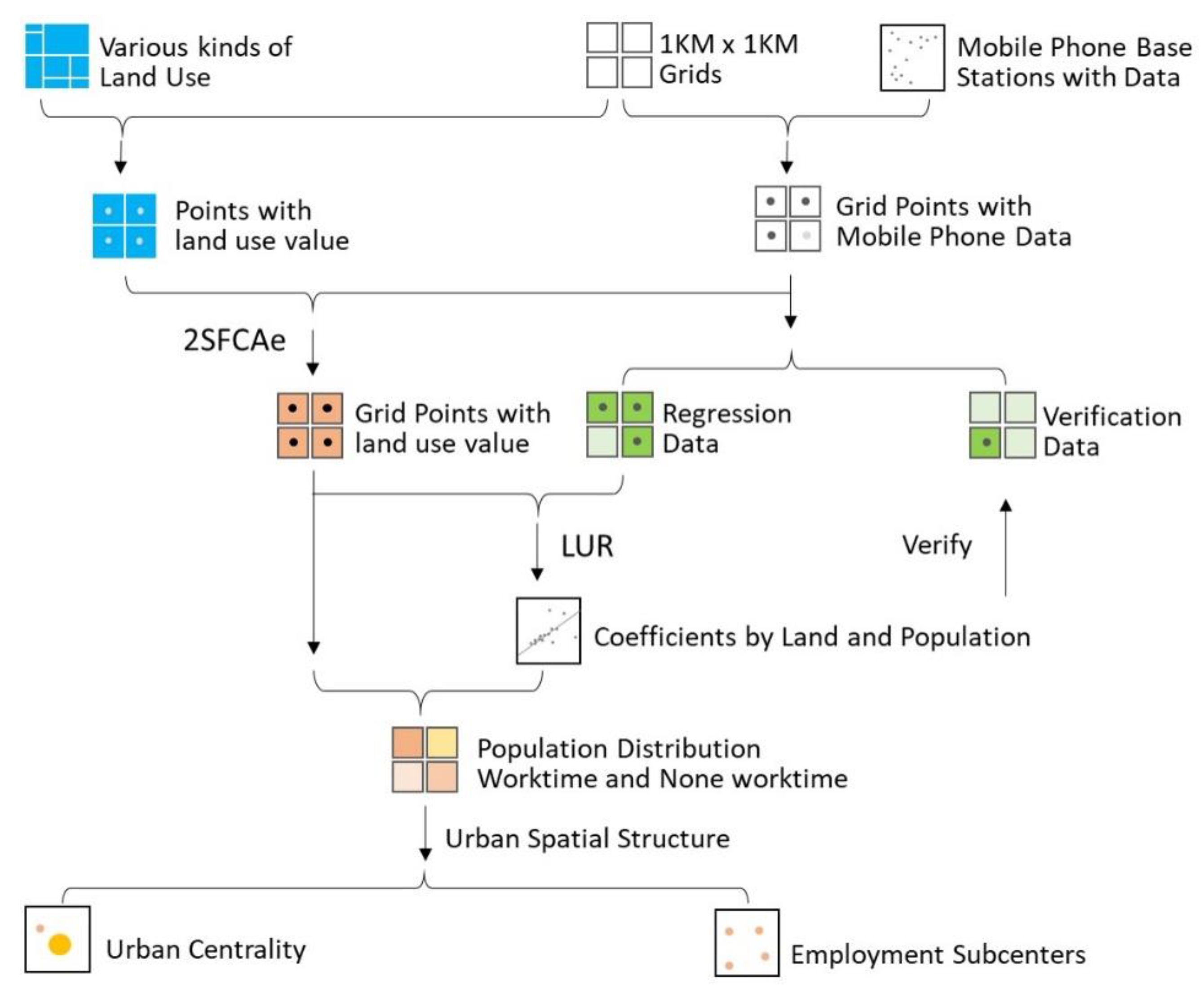
The major workflow of the study is presented in Figure 4. The major steps are: (1) Create the 1 km × 1 Km grid and centroids in study area to represent users population of mobile phone base stations inside and the land area of various kinds of land use. (2) Apply the 2SFCAe method to assign grid points with land use value. (3) Implement LUR with population and land use value to verify the regression fit by substituting coefficients to verification data. (4) Substitute coefficients back to grid points with land use variables to acquire the population distribution in worktime and non-worktime, based on which urban spatial structure was explored. The main procedure is the 2SFCAe model.

3.1. Land Use Regression Model

Land use regression model is a multi-variable linear regression model, prevalently utilized for urban air pollution modeling with four elements: observed data, geographic predictors, model development and validation [24], offering pollution mapping of higher resolution compared to traditional interpolation methods. With a connection and regression between geographic elements and part of monitoring data, LUR sets a linear equation with coefficients for corresponding geographic variables, verifies equations with the rest monitoring data by substituting coefficients back, and then assigns the value to space around the observation spots.

People commonly rest in residential areas, and work in offices, commercial and industrial zones; land uses surrounding base station directly relate to the size of mobile phone user’s population. LUR model can interpolate the size of mobile phone population to the surrounding land uses, which has the same equation as the traditional form in air pollution studies:

Y_i = k₀ + k₁x₁ + k₂x₂ + …… + k_nx_n + ε_i

(1)

where Y_i is the population number provided in mobile phone data of base station i, K₀ is a constant as intercept, x_n is the value of type n land use surrounding base station i with a corresponding coefficient K_n, and ε_i is the random error.

In contrast, Y_i is a summarized value of adjacent area other than density value applied in LUR models of air pollution, constituting a similar demand–supply relation between population value of base station and nearby lands, which make 2SFCA method employed in accessibility studies appropriate for combination with LUR.

3.2. Two-Step Floating Catchment Area with Entropy Gravity Method

As the prototype of 2SFCA, Floating Catchment Area method (FCA) merely considers land use effects around observation point as most of traditional LUR models have done. Both models consider the distance threshold and decay effect, yet ignore spatial heterogeneity as base stations with the same land use pattern may differentiate in population for their different spatial location such as CBD and subcenters. 2SFCA takes land influence into account with a weighted approach of population as a reflection of spatial heterogeneity, which means that the larger the population of the base station is, the larger that of surrounding land is as well, though the corresponding land value may be the same.

The basic ideas underlying 2SFCA is that the supply and demand points are used as centers to perform floating catchment searches, respectively. For the first search, public facility (j) is used as the center point, all settlements (k) within a threshold distance (d₀) are searched. Thus, the ratio (R_j) between the service capacity of the facility and the served population within the corresponding area is calculated. For the second search, each settlement (i) is used as the center point, all locations of public facilities within a threshold distance (d₀) are searched. The aggregated services (R_j) from various public facilities are summarized to acquire the service capacity of a public facility (accessibility) at point (i).

Despite its relative popularity, the 2SFCA method still has its limitation for its dichotomy, determining accessibility value merely according to a fixed threshold distance (or time). Some studies have constructed a distance decay effect model using a kernel density function, gravity model or Gaussian function. As a summarization to which, Wang presented G2SFCA model with an integrated equation about decay function f(d) and illustrated the different pattern as follow: (a) Gravity function; (b) Gaussian function; (c) 2SFCA; (d) E2SFCA; (e) Kernel; and (f) three-zone hybrid approach [30].

$$A_i={\sum }_{j=1}^n\left[{\mathrm{S}}_j\mathrm{f}\left(d_{ij}\right)/{\sum }_{k=1}^m{\mathrm{p}}_k\mathrm{f}\left(d_{kj}\right)\right]$$

(2)

As new physics holds that gravity is a kind of entropic force [31], this article takes Wilson’s entropy gravity model as decay effect pattern in 2SFCAe. Wilson deduced an interactive model based on the principle of Maximum Entropy rather than a metaphor of Newton gravity model [32], changing the interaction equation from power function to exponential function:

T_ij = A_iO_iB_jD_jexp(−βC_ij)

(3)

The difference between them is that the Newton power function is more sensitive to the reduction of distance. As the distance becomes greater, the difference becomes smaller.

With a simplification to Wilson Entropy Gravity model, this article defined the gravity value between O_i and D_j as T_ij = O_iD_jexp(−2d_ij), giving the coefficient β value of 2 as most traditional gravity function does.

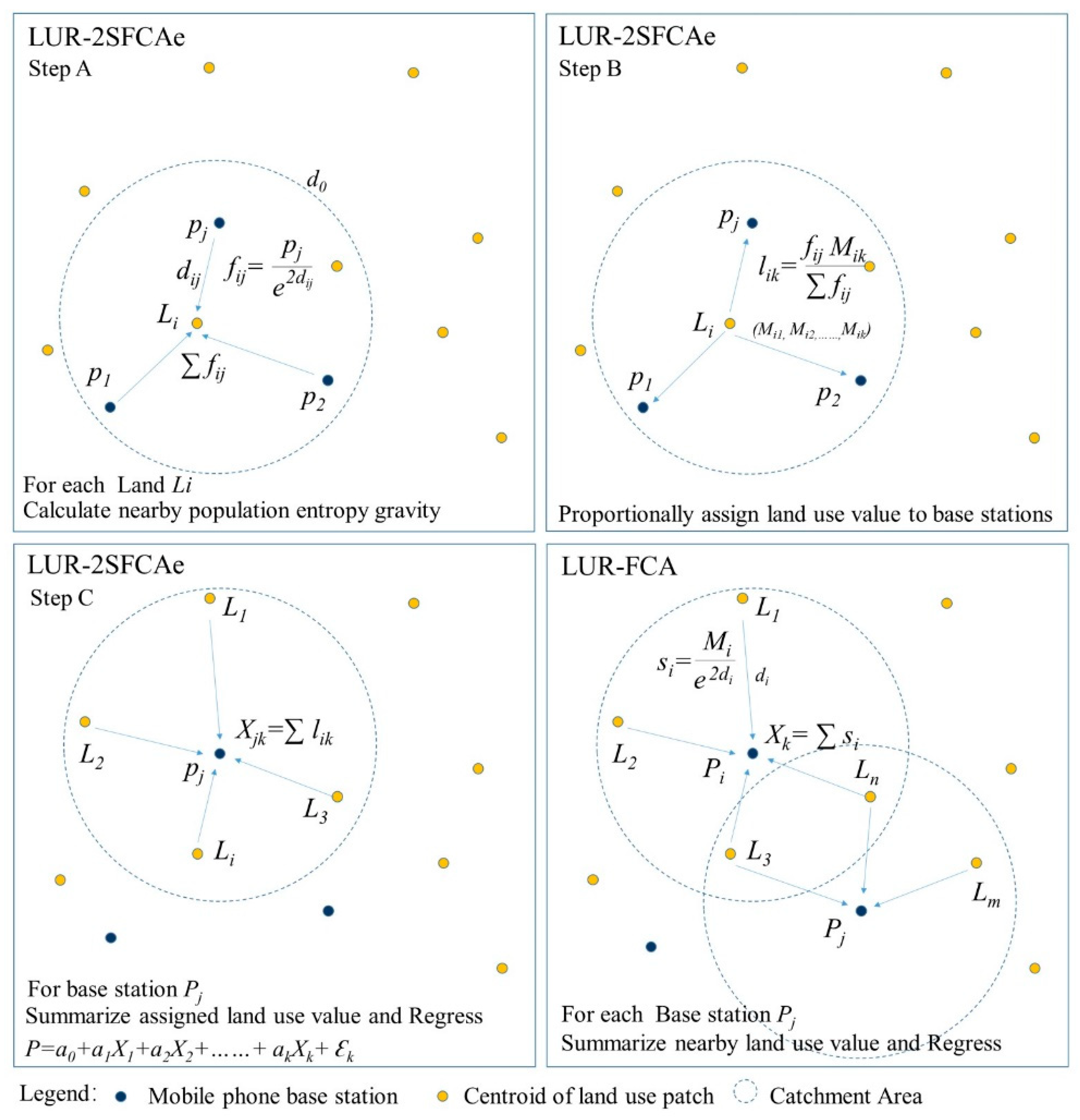
3.3. LUR-2SFCAe Method

As mobile phone base station j with population p_j, land point L_i with k different types of land use of corresponding area value (M_i1, M_i2, ……, M_ik) and the distance between them as d_ij, the procedures of LUR-2SFCAe are as follows:

(1) Calculate the population entropy gravitational value for each piece of land L_i, and the surrounding j base stations (population p_j) within the threshold range d₀:

f_ij = p_j*exp(−2d_j) ∀d_j ≤ d₀

(4)

(2) Aggregate population gravitational entropy for each land point L_i: ∑f_ij;

(3) Assign land value back of L_i (M_i1, M_i2, ……, M_ik) to surrounding base stations proportionally:

l_ik = M_ik*f_ij/∑f_ij

(5)

(4) Summarize the total land value of base station j assigned by surrounding land points within the threshold range d₀:

X_jk = ∑l_ik ∀d_j ≤ d₀

(6)

(5) Explore a linear regression function with all population p_j and its land value set (Xj₁, X_j2, ……, X_jk) of base stations as P = f (X_k):

P = a₀ + a₁X₁ + a₂X₂ + a₃X₃ + ...... + a_kX_k + ε_k

(7)

where X_k is a set of land value of different types, a_k is the corresponding coefficient, a₀ is the constant and ε_k is standard error.

(6) Verify the reliability of the regression model with verification data of base stations, substitute the regression coefficient back to calculate the total population of land point L_i.

The illustration of the regression model for LUR-2SFCAe and a comparison with FCA method is as follows (Figure 5):

4. Results

4.1. Regression Result of LUR-2SFCA

This study defined the search threshold as 5000 m, larger than most of buffering zone of LUR in air pollution studies, taking most of Land use types into account as R (Residential), A (Administration and public services), B (Commercial and business facilities), MW (Industrial, logistics and warehouse), U (Municipal utilities), G (Green space and square), S (Road, street and transportation), H1 (Town and country), H2 (Regional infrastructure), E1 (water) and E2 (Farmland) and all-time population. While some of the base stations and land point overlay in same grids, between which the interaction distance is defined as 200 m.

Performed 2SFCAe with previous land use data and all-time population, and then a stepwise regression in SPSS, the regress retains the following six parameters, R, A, B, MW, H1, and E with a final adjusted R² of 0.792, showing a high fitness of LUR-2SFCAe model (

Table 1. Summarization of stepwise regression (all-time).

Model Summary
Model	R	R2	Adjusted R2	Std. Error of the Estimate	Predictors
1	0.821	0.674	0.674	3208.54425171590500	(Constant), R
2	0.852	0.726	0.726	2942.90174974674660	(Constant), R, A
3	0.875	0.765	0.765	2725.59070375458400	(Constant), R, A, B
4	0.883	0.780	0.779	2641.12225592935500	(Constant), R, A, B, MW
5	0.887	0.786	0.786	2603.89655684452830	(Constant), R, A, B, MW, H1
6	0.890	0.792	0.792	2566.13576819830540	(Constant), R, A, B, MW, H1, E1

). It could also be concluded that residential zone played a dominant role in population distribution, then public service, commercial, industrial, logistics and warehouse in the main urban area, town and country and water in the regional background.

For exploring the urban spatial feature, this experiment implements regression with the population of worktime and non-worktime to get population distribution in different periods. As compared with all-time population, non-worktime displays a higher adjusted R² of 0.82 while worktime shows the same (

Table 2. Summarization of regression (worktime and non-worktime).

SUMMARY OUTPUT
Regression Statistics (Worktime)				Regression Statistics (Non-Worktime)
Multiple R		0.890264		Multiple R		0.906303421
R Square		0.792571		R Square		0.82138589
Adjusted R Square		0.791919		Adjusted R Square		0.820904883
Standard error		2564.744		Standard error		2370.731631
Observation		2235		Observation		2235
ANOVA	(worktime)
	df	SS	MS		F	Significance F
Regression	6	5.6 × 1010	9.33 × 1010		1416.09	0
Residual	2228	1.47 × 1010	6,585,053
Total	2234	7.06 × 1010
ANOVA	(non-worktime)
	df	SS	MS		F	Significance F
Regression	6	5.76 × 1010	9.6 × 1010		1707.636	0
Residual	2228	1.25 × 1010	5,620,368
Total	2234	7.01 × 1010

).

Comparing coefficients with non-worktime (

Table 3. Regression Coefficients (worktime and non-worktime).

Worktime	Coefficients	Standard Error	t Stat	p-Value
Intercept	477.8392	80.59048	5.929226	3.52 × 10−9
R	0.018144	0.000499	36.33294	2.1 × 10−227
A	0.017012	0.000819	20.77093	9.65 × 10−88
B	0.039378	0.001912	20.59004	2.24 × 10−86
MW	−0.00431	0.00036	−11.9656	5.04 × 10−32
H1	0.002634	0.000228	11.56714	4.3 × 10−30
E	−0.00016	1.97 × 10−5	−8.19038	4.34 × 10−16
Non-Worktime	Coefficients	Standard Error	t Stat	p-Value
Intercept	454.0856	74.45374	6.098896	1.26 × 10−9
R	0.02138	0.000461	46.34211	0
A	0.0149	0.000757	19.6916	1.04 × 10−79
B	0.029965	0.001767	16.95971	9 × 10−61
MW	−0.0051	0.000333	−15.3391	1.47 × 10−50
H1	0.00256	0.00021	12.16957	4.92 × 10−33
E	−0.00016	1.82 × 10−05	−8.51949	2.9 × 10−17

), worktime has larger amounts in intercept, A, B, WM and H1 type land, which provides job opportunities, while it has a smaller amount in R land and shares the same amount in E.

By substituting the coefficients back to LUR equation, the rest of the mobile phone data were verified with the corresponding population with a resulting R² of 0.897, which confirmed the applicability of LUR model, then the population of every land points could be computed as well in worktime and non-worktime.

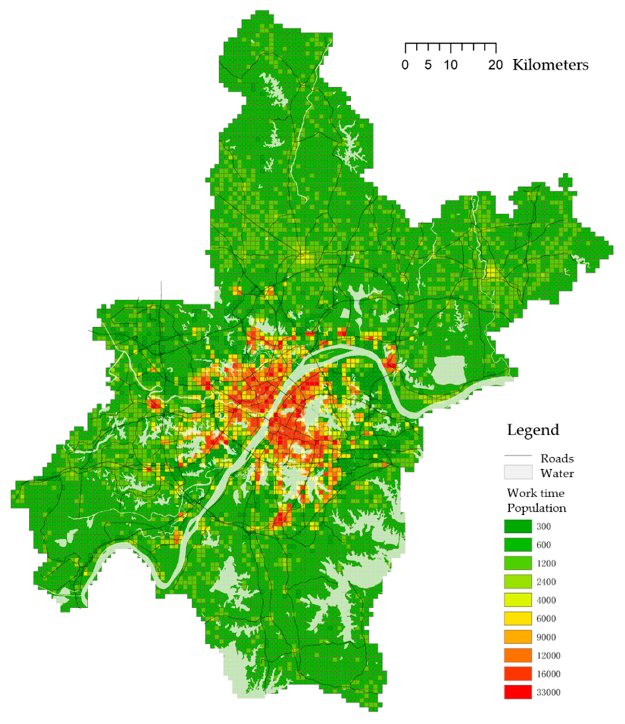
4.2. Exploring Spatial Feature with Gridded Population

Resubstituting the coefficients to the equation can generate the population. As the population is computed by the regression equation with the land entropy gravity, the value is not a direct output but proportional to the actual population of the cells. Plotted with the population of the whole 8999 cells of worktime and non-worktime in ten levels with natural breaks in ArcGIS (Figure 6), both population distribution maps with a similar hierarchical distribution, clearly distinguish the waters, especially in the central area, showing higher accuracy as compared to other interpolation methods such as Kernel, Kriging, etc.

From the density pattern, Wuhan shows a multi-nuclei model in spatial structure with an obvious dominant and compact core in the main city and several sub-cores around its periphery mostly located across the waters. Such natural environment as rivers and lakes impose strong constraints on the structural development of Wuhan which expanded mostly along the waters and roads. In general, urban spatial form and pattern of Wuhan are affected and limited by natural environments.

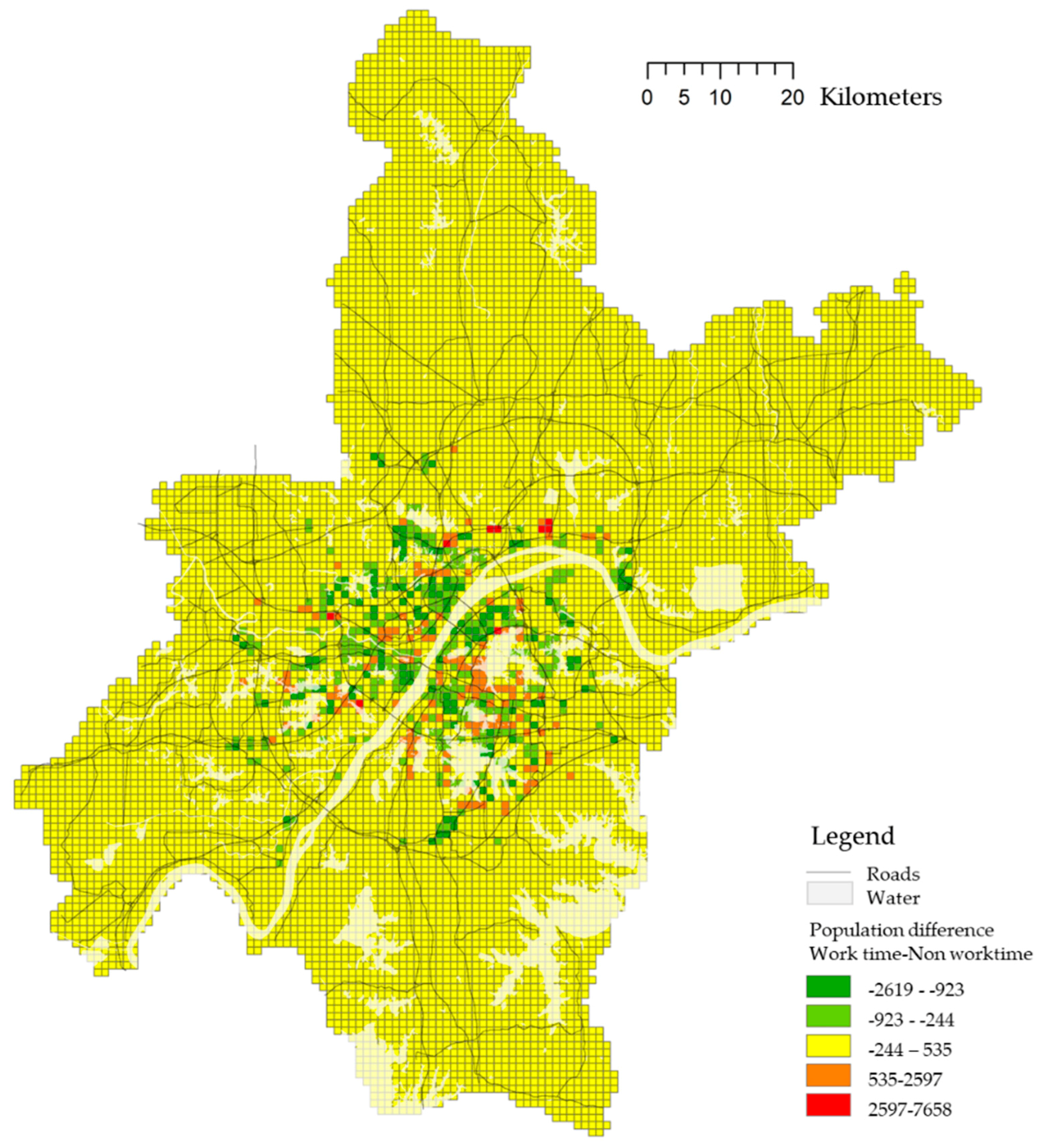
The population difference between worktime and non-worktime can represent the characteristics of each land distinguished as employment center or residential area, in that, if the worktime population is greater than non-worktime, it will be the employment center, otherwise, it is a residential area. Mapping the population variance in ArcGIS with five groups and Jenkin’s breaks, most of the cells outside the main city were in middle level, reflecting a natural metropolis boundary of Wuhan, wherein the larger positive numbers are the employment centers and smaller negative numbers are the residential areas (Figure 7).

With a relatively compact employment cluster in the central area, the urban spatial structure shows a trend of sprawling to the outskirts, especially in the north along the Yangtze River and in the east. The phenomenon that employment center grows on the periphery reflects the characteristics of top-down urbanization driven by the governments in China. The planning led by the governments also has a greater impact on an intentional move out of the industrial park, universities, colleges, and commercial wholesale market from downtown to periphery under the policy of land finance [33].

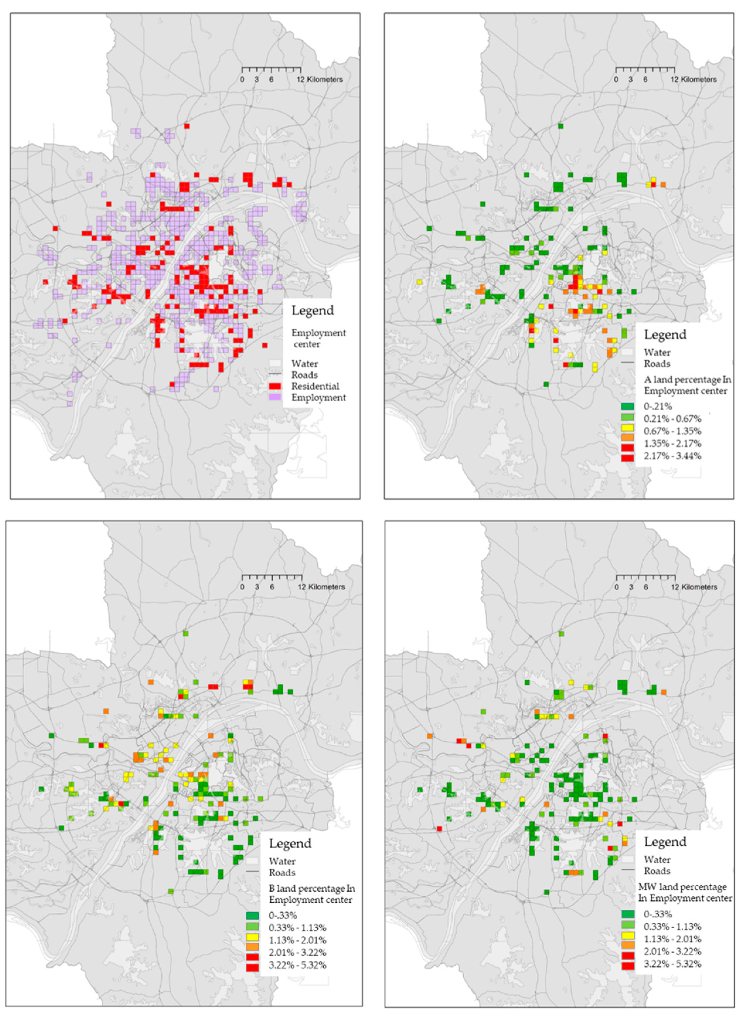
Since land types A, B, and WM play important roles in worktime population, the conclusion is drawn from the regression above that the percentage of different types of land uses in units can be analyzed to show the distribution of different categories of employment centers.

When mapped in ArcGIS (Figure 8), most of the employment centers of A land are located in Wuchang District which has many universities and research institutes, those of B land situate in Hankow District which is a historical commercial district, and those of WM land disperse around the outskirts. The universities and markets around the outskirts are a result of planning by the government which relocated them to the suburbs intentionally for a density evacuation in the central city, a motivation for urban sprawling and a result of the land economy pursuit.

As compared with the traditional concentric model, sector model and multi-nuclei model, Wuhan shows a mixed pattern: a dominant center and several minor sub-centers of different functions, expanding along the river or traffic corridors.

5. Discussion

These results suggest that LUR-2SFCAe is fit for dasymetric mapping with mobile phone data and to present land uses, wherein the distance decay setting of 2SFCAe tackles the problem of the undefined boundary of base station service area. These findings are understandable because there exists certain connection between user population of mobile phone base stations and surrounding land uses.

These results agree with Anto’s findings [26] that mobile phone data reflect surrounding population density. The regression R² in this experiment is higher than that reported in Image Texture method [13], and similar to building population mapping with PopShape GIS [34], which further verify the conclusion of Bakillah [20] that finer scale ancillary data provide more accurate dasymetric mapping. Furthermore, 2SFCAe method explores the distance-decay function and weighted population effect in interpolation which can be seen as an improvement of kernel density surface method with population-weighted census centroids [35], and is better than FCA method, as in public service studies [36].

As a comparison of the assumption of gridded mobile phone data and the uncertainty in boundary issue, this study also applied the same LUR-2SFCA method on original mobile phone data and explored LUR with Thiessen polygon boundary of base stations. Both regressions showed a lower R². While LUR-2SFCAe was tested and calculated with all-time population of original mobile phone data and land use data, the regression result in SPSS (

Table 4. Summarization of Regression with original mobile phone data.

Model Summary
Model	R	R Square	Adjusted R Square	Std. Error of the Estimate	Predictors
1	0.080	0.006	0.006	323.201	(Constant), R
2	0.115	0.013	0.013	322.084	(Constant), R, H1
3	0.120	0.014	0.014	321.899	(Constant), R, H1, MW

) retained only three parameters as R, H1 and MW, showing an unacceptable R² which indicates the data or model need to be modified. Meanwhile, when Thiessen polygons were applied on original base stations, the regression with user population and the land uses inside the polygons retained similar parameters as previous models and a same low R² (

Table 5. Summarization of Regression with Thiessen Polygons.

Model Summary
Model	R	R Square	Adjusted R Square	Std. Error of the Estimate	Predictors
1	0.164	0.027	0.027	896.784	(Constant), R
2	0.182	0.033	0.033	894.020	(Constant), R, A
3	0.192	0.037	0.037	892.199	(Constant), R, A, H1
4	0.200	0.040	0.039	890.932	(Constant), R, A, H1, E1
5	0.206	0.042	0.042	889.737	(Constant), R, A, H1, E1, MW

).

The interesting thing is that the Thiessen polygons method does not considered spatial heterogeneity, unlike many traditional methods [21], since different polygons may contain the same land use components but vary in user population. However, the former has verified the unevenness in spatial heterogeneity as nearby station may have different population. Although the 1 km grid was applied in this study with a persuasive regression result, a balance of unevenness and heterogeneity remains to be explored for finer-grid mapping.

These results provide substantial evidence for the assumption that the combination of LUR and 2SFCA can map population with mobile phone data and land use, which addresses the spatial heterogeneity in most dasymetric mapping, and tackles the problem for the undefined boundary of base stations in 2SFCA. Furthermore, the 2SFCAe defines a new demand–supply model comparing with traditional LUR model which often simply summarizes the land use of its buffering zone.

6. Conclusions

This paper develops a methodology of LUR-2SFCA with mobile phone data and land use data to alleviate the spatial heterogeneity issue which challenges most dasymetric mapping methods and explore urban spatial feature with population mapping of different time at finer scale. As a result of the experiments, it is concluded that mobile phone data reflect more temporal, detailed and accurate population than census data. Furthermore, the distance-decay model in 2SFCA can solve the uncertain service boundary issue of mobile phone base station and its user population. Additionally, the 2SFCA assigns a weighted population to nearby land patches which again strengthens the spatial heterogeneity of observed population, hence improving the fitness of regression. Finally, the work-time and non-worktime population distribution calculated by LUR-2SFCAe can help identify urban centrality and employment centers.

On the other hand, based on comparison of original mobile phone data and Thiessen polygon method, spatial heterogeneity and unevenness of mobile phone data are supposed to affect the outcome of dasymetric mapping, which needs to be further studied.

Although land use and mobile phone data utilized in this paper can provide population mapping of a relatively high resolution, both data types could only be acquired locally, which may limit their implementation on a global scale. On the other hand, this method might face the challenge of computation due to the sizes of grids and floating catchment area, when the grids are smaller and the spatial resolution finer. The calculation task will increase exponentially in the procedure of distance calculation within a floating catchment area, which might exceed the calculation capability of the computer or related software.

In general, the contribution of the present study lies in the methodology combination of LUR and 2SFCAe, which provide a distance-decaying demand–supply model in dasymetric mapping with mobile phone data and land use data. The methodology of LUR-2SFCAe is also applicable to related dasymetric mapping and LUR studies.