Hydrological Evaluation of Flow Diversion Terraces Using Downhill-Slope Calculation Method for High Resolution and Accuracy DEMs

Abstract

Slope is an important topographical parameter in hydrological models. Dramatic changes in slope are produced due to micro variations of topography in flow diversion terrace (FDT) systems. Assessing the effectiveness of FDT on soil conservation yields different results using different slope calculation methods with different resolution and accuracy digital elevation models (DEMs). In this study, the ArcGIS built-in average-neighborhood-slope (ANS) method and a downhill-slope (DHS) method were used to calculate slopes for a small agricultural watershed in New Brunswick, Canada. Six DEMs were used, i.e., 1, 5 and 10 m resolution DEMs generated with conventional photogrammetric techniques, and 1, 5, and 10 m resolution DEMs derived from light detection and ranging (LiDAR) data. Calculated slopes were summarized for the whole watershed, a patch of FDT systems, and grassed flow channels in front of embankments in the patch. Results indicated that the DHS method produced smaller slopes than the ANS method with LiDAR-1m DEM along grasses flow channels. Furthermore, the mean L-factor derived from the DHS method was smaller than that derived from the ANS in terraces and grassed flow channels for the LiDAR-1m DEM. Finally, soil loss estimated from the DHS method using RUSLE was more consistent with measurement for the watershed than that from the ANS method when the LiDAR-1m DEM was used. The DHS method can provide accurate slopes along grassed flow channels and can be used to assess FDT systems using USLE-based models with high resolution and accuracy DEMs.

1. Introduction

Assessing the effectiveness of a flow diversion terrace (FDT) system is of importance for landowners and agricultural agencies to make decisions. Benchmarking or paired watersheds, upstream and downstream monitoring, and edge-of-field testing can help determine the efficiency of the FDT [1]. However, when it comes to large agricultural areas the experimental survey is time-consuming and expensive [2,3]. Thus, effective assessing tools such as hydrologic models are necessary for evaluation of the impact of FDT on soil conservation. USLE (universal soil loss equation)-based soil loss prediction algorithms are the most widely accepted and utilized method in hydrological models, such as in the Soil and Water Assessment Tool (SWAT) [4]. In those USLE-based algorithms soil conservation support practice factor (P-factor) is often required as an input to estimate the effectiveness of FDTs. Many studies have pointed out that large uncertainty was associated with those monitored P-values [5,6,7]. These P-factor values are limited to applications of USLE-based methods at a specific field in which a FDT system is imbedded. This limitation stemmed from the intrinsic characteristics of USLE-based methods which are developed based on numerous experiments at field scale. The P-factor values for various FDT implementations are only valid when the size of a field is greater than that of a FDT system.

With the advance in Geographic Information System (GIS) technique in the past few decades, application of USLE-based methods has been extended to grid cell scale defined by digital elevation models (DEMs). With the resolution of DEMs getting greater, the size of grid cells generally smaller than an agricultural field. Thus, the P-factor values defined from experiments are not reliable when USLE-based methods are employed at the grid cell scale to assess soil conservation effects of FDT systems. Therefore, the major benefit associated with the implementation of FDT systems should be reconsidered. In fact, the conservation effects of FDT systems are the result of reducing slope length and slope angle in front of embankments, which are represented by L and S-factor (combined as LS-factor) in USLE-based methods, respectively [8].

With high resolution and accuracy DEMs available, the LS-factor of USLE-based models can be derived directly for FDT systems. Consequently, the method to calculate LS-factor with high resolution and accuracy DEMs should be revisited to supply better techniques for estimate soil erosion in croplands. Studies showed that the LS-factor is determined by the slope when USLE-base methods were applied in GIS environment [9,10,11]. The built-in method in ArcGIS to calculate slopes is the average-neighborhood-slope (ANS) method. The ANS method estimates slopes by calculating the rate of altitudinal change over the distance from the central cell to its eight neighboring cells using an average maximum technique [12]. This method can provide accurate slopes for gently variating landscapes with low resolution and accuracy DEMs (which cannot detect embankments of a FDT system), while for high resolution and accuracy DEMs (e.g., 1 m resolution LiDAR DEMs), it may fail to accurately account for micro-variations in FDT systems. Thus, a reliable slope calculation method is required for high resolution and accuracy DEMs to correctly estimate LS-factor and, as a result, the effectiveness of FDT systems can be accurately evaluated using USLE-based methods.

The objectives of this study are to: (1) introduce a new slope-calculation method for high resolution and accuracy LiDAR DEMs; (2) compare the built-in and new slope-calculation methods in calculating slopes for FDT systems with different resolution and accuracy DEMs at watershed, terrace, and flow channel scale; (3) evaluate LS-factors and soil losses calculated based on two different slope-calculation methods.

2. Research Background

Flow diversion terrace systems implemented in agriculture watersheds are effective best management practices (BMPs) for soil conservation [1]. A typical FDT system consists of graded parabolic channels and earth embankments constructed across the slope to disrupt long slopes with shorter segments [13]. The FDT can reduce surface runoff and energy in the transportation of detached soil particles which deposit in grassed flow channels in front of embankments. Because of shorter slope length, FDT can reduce sheet and rill erosion on croplands and reduce sediment delivery by deposition, trapping much of the sediment eroded from areas between the diversion embankments [13]. With FDT systems in place, deposited sediments remaining on site can be redistributed over the field by ploughed fallow and tillage.

The P-factor is defined as the ratio of soil loss with a soil conservation practice in place to the soil loss without soil conservation [8]. It is a quantitative indicator reflecting the reduction of soil erosion associated with the implementation of BMPs that alter flow patterns, grade, or direction of surface runoff. Recommended P-factor values for virous BMPs are based on experiments and generalized in the USDA handbook 537 [8].

The idea of extending the LS-factor to three-dimensional form, to include topographic effects is important in erosion estimation when DEMs are considered. Using upslope contributing area per unit width for overland flow to calculate LS-factor was first theoretically proposed by Moore and Burch [14]. They found that theoretically derived LS-factor was equivalent to empirically derived counterpart in the USLE. The theoretically based LS-factor was physically based and better accounted for three-dimensional hydrological and topographic effects associated with converging and diverging terrain [15]. A method of LS-factor extraction from a DEM based on the concept of unit contributing area has been presented by Desmet and Govers [16]. They extended the Foster and Wischmeier [17] approach to calculate LS-factor and found that the algorithm would increase the applicability of USLE-based methods in a GIS environment allowing for the calculation of LS-factor on a grid cell basis.

Resolution and accuracy of DEMs from different sources have great impacts on estimation accuracy of hydrologic parameters such as LS-factor. Conventional DEMs for large areas obtained by photogrammetric method is widely used, though there are many problems such as ridging phenomenon of DEMs [18]. High resolution and accurate DEMs obtained by light detection and ranging (LiDAR) have been used in deriving hydrologic parameters and proved to improve the quality of those parameters. As the dimensions of FDT are generally smaller than the resolution of most conventional DEMs, it is generally inaccurate to estimate the LS-factor from conventional DEMs.

3. Materials and Methods

3.1. Study Area

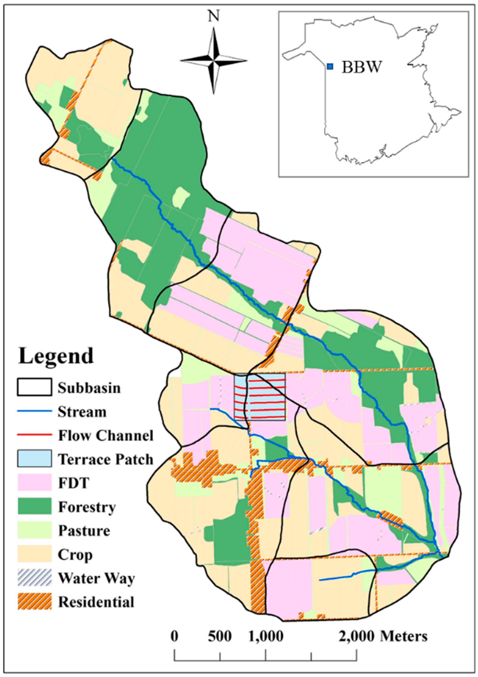
The study was carried out in the Black Brook Watershed (BBW), located in the northwest New Brunswick (NB, 47°05′–47°09′ N, 67°43′–67°48′ W), Canada (Figure 1). The watershed has been studied extensively for evaluating the impact of agriculture on soil erosion and water quality for near 30 years [19,20]. The watershed covers an area of 14.5 km², with 65% of its land use is in agriculture, 21% in forest, and 14% in residential areas and wetlands [21]. Elevations range from 170 to 260 m above mean sea level [22]. Slopes vary from 1–6% in the upper basin to 4–9% in the central area [23,24]. In the lower portion, slopes are more strongly rolling at 5–16%. The climate of the region is considered to be moderately cool boreal with approximately 120 frost-free days [2]. The average temperature is 3.7 °C and annual precipitation is 1037.4 mm [21,25,26]. About one-third of the precipitation is in the form of snow. Snowmelt leads to major surface runoff and groundwater recharge events from March to May [20].

The major crop is potato, grown on about 33% of the BBW production area, followed by grain, peas, and hay in rotation. Soil erosion has been a serious problem in potato growing areas in New Brunswick including the BBW. To mitigate soil erosion induced water quality degradation, various BMPs have been adopted in the BBW. Starting from early 1970, variable grade flow diversion terraces has been constructed to reduce soil erosion. Until 2011, more than half of the agricultural area was protected by FDT systems (Figure 1) [24].

3.2. NBGIC and LiDAR DEMs

The conventional DEM was obtained by the photogrammetric method from 1:35,000 aerial photographs. The original distance between the regenerated irregular elevation points was 25 to 70 m [18] and they were interpolated into 1, 5, and 10 m grid with the inverse distance weighting (IDW) method using ArcGIS. Those DEMs were referred as NBGIC-1, 5, and 10 m DEM in the study. The original LiDAR data has horizontal accuracy of 0.5 m and the vertical accuracy was less than 0.15 m. After eliminating non-ground points, a 1 m resolution DEM was generated by means of the IDW method [18]. This was labelled as LiDAR-1m DEM. By re-sampling the LiDAR-1m DEM, 5 and 10 m resolution DEMs, i.e., LiDAR-5 and 10 m DEM, were generated.

3.3. Revised Universal Soil Loss Equation

In the present study, we employed the revised uniserial soil loss equation (RUSLE) to estimates average annual soil loss based on soil characteristics, topography, climatic conditions, land use, and support practices (USDA-ARS, 2008), i.e.,

A_i = R_i K_i L_i S_i C_i P_i

(1)

where,

• A_i is the estimated average annual soil loss for ith cell (t ha⁻¹ year⁻¹);
• R_i is the rainfall erosivity-factor (MJ mm ha⁻¹ h⁻¹ year⁻¹);
• K_i is the soil erodibility-factor (t h MJ⁻¹ mm⁻¹);
• L_iS_i is the slope length and steepness factor (LS-factor);
• C_i is the cover management-factor; and
• P_i is the support practice-factor (P-factor).

Values for the R, K, and C-factors were estimated based on the method outlined by Wall, et al. [27]. P-factor was assumed to be equal to 1. Following Moore and Burch [14], Moore and Wilson [28], and Desmet and Govers [16], the L and S-factors were calculated from Equations (2) and (3), respectively,

L = (A/22.13) ^0.4

(2)

S = (sin β/0.0896) ^1.3

(3)

where:

• A is upland contributing area; and
• β is the slope angle (%).

Upslope contributing area was computed from the sum of grid cells from which the water flows into the cell,

$$A=\frac{1}{b}{\sum }_{i=1}^n{u}_i{a}_i$$

(4)

where

• ${\alpha }_i$ is the area of ith grid cell;
• n is the number of cells draining into the grid cell;
• ${\mu }_i$ is the weight depending on the runoff generation mechanism and infiltration rates; and
• b is the contour width approximated by the cell resolution [9].

In this study, we used the data of 2000 to calculate erosivity in BBW. The precipitation in 2000 was 1098 mm, and the erosivity was 1242 MJ mm ha⁻¹ h⁻¹ year⁻¹ for the BBW. The measured sediment yield in 2000 was 3211 t year⁻¹. RUSLE was used to calculate soil losses in BBW with different resolution and accuracy DEMs and results were summarized for the entire study area and a patch of a FDT system on cropland (Figure 1).

3.4. Slope Calculation

Two slope-calculation methods were applied at three different resolutions (i.e., at 1, 5 and 10 m resolutions) and two accuracies (i.e., conventional photogrammetric method and LiDAR). The results were summarized for the whole watershed, a terrace patch, and 1 m-buffer zones in front of embankments (i.e., greased flow channels) within the patch.

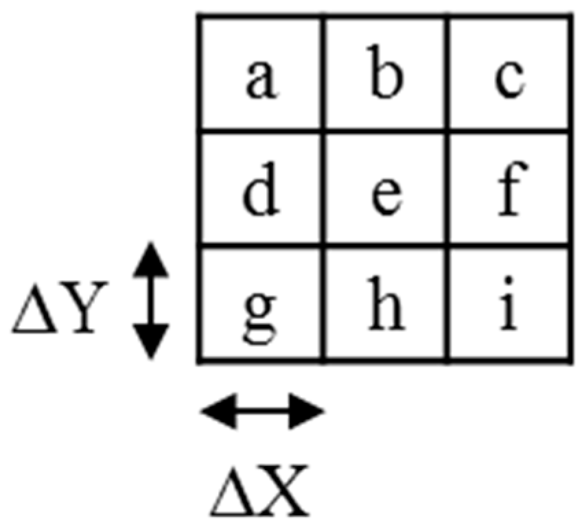
The ANS method conceptually creates a surface of 3 × 3 neighboring cells to determine the average rate of change in elevation along the horizontal direction (dZ/dX) and lateral directions (dZ/dY) from the central cell (cell e; Figure 2):

$$\mathrm{ANS}(\mathrm{e})=\mathrm{Arctan}\left(\sqrt{{\left(\frac{\mathrm{dZ}}{\mathrm{dX}}\right)}^2+{\left(\frac{\mathrm{dZ}}{\mathrm{dY}}\right)}^2}\right)$$

(5)

where:

• $\frac{\mathrm{dZ}}{\mathrm{dX}}$ = ((Z_c + 2∙Z_f + Z_i) – (Z_a + 2∙Z_d + Z_g))/(8∙∆x) and
• $\frac{\mathrm{dZ}}{\mathrm{dY}}$ = ((Z_g + 2∙Z_h + Z_i) – (Z_a + 2∙Z_b + Z_c))/(8∙∆y),

with Z_{j=a...i, ≠e}, as the elevation of the eight surrounding cells. ∆x and ∆y specify the cell dimensions in the horizontal and lateral directions, respectively (Figure 2). Typically, ∆x = ∆y to simplify grid representation and associated evaluations.

The downhill-slope (DHS) method is introduced and described by Ashraf, et al. [29]. The DHS method provides a more intuitive description of surface water flow characteristics in uneven terrain. The DHS method calculated slope (in degrees) from a central cell (cell e; Figure 2) in one of eight directions with maximum elevation drop [30]:

$$\mathrm{DHS}(\mathrm{e})=\mathrm{Arctan}\left[\max \left(\frac{{\mathrm{Z}}_{\mathrm{e}}-{\mathrm{Z}}_{\mathrm{j}}}{{\mathrm{L}}_{\mathrm{j}}}\right)\right]$$

(6)

where:

• L_j = Δx, when j = b, d, h, and f in the orthogonal direction,
• L_j = 1.414 Δx, when j = a, c, g, and i in the diagonal direction,

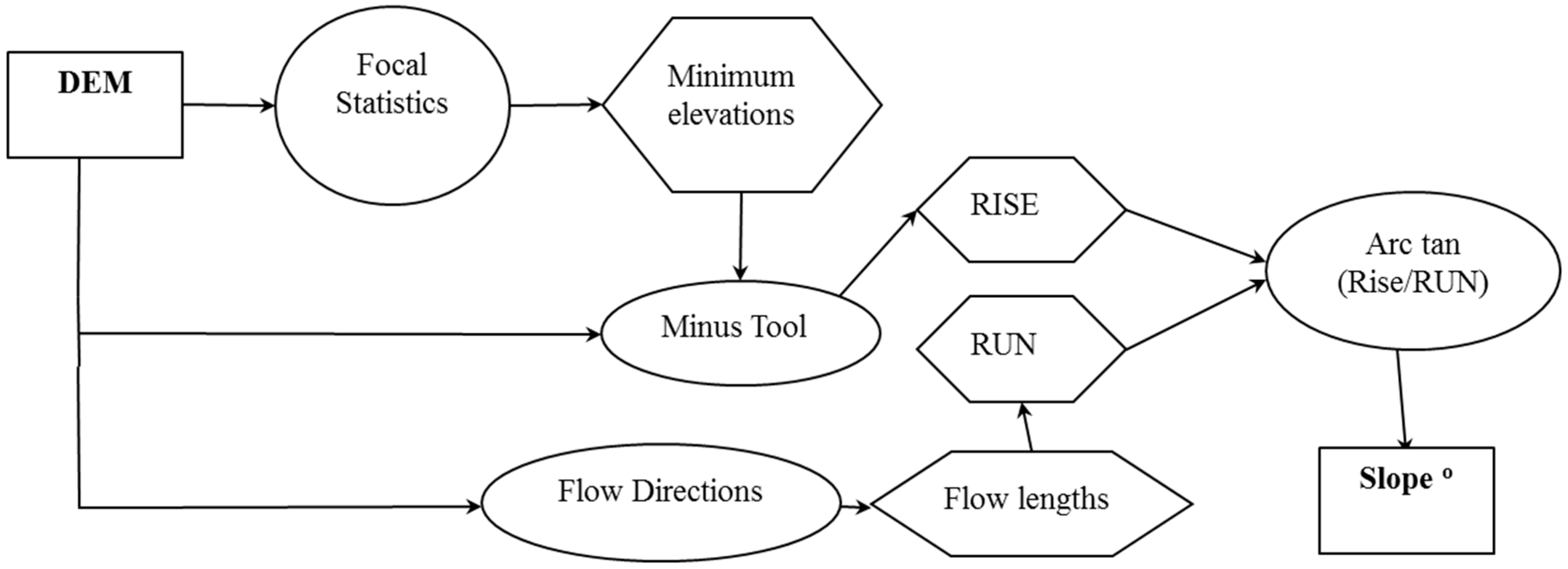
and Z_e is the elevation of the central cell and Z_j is the elevation of one of the eight surrounding cells that gives the maximum drop (Figure 2). Specifically, following Figure 3, the “focal-statistic” tool in ArcGIS was used to estimate the maximum elevational difference between the central cell and the eight surrounding cells so that the 3 by 3 rectangular neighborhood kernel was utilized. The “flow-direction” tool to determine whether the downhill flow is diagonal or orthogonal in the calculation of horizontal distance.

3.5. Slope Length Cut-Off Value

Since concentrated flows develop when the hill slope is long and uninterrupted, a slope length limit is normally determined to represent the scale at which the inter-rill and rill erosion occur [31]. Apparently, slope length limit varies from site to site and from watershed to watershed depending upon topography, soil characteristics, climatic conditions, and agricultural activities. An arbitrary slope length cut-off value can lead to poor estimation of soil loss. Several studies have been carried out to solve this problem [9,10,11]. In the present study, we employed the cut-off slope angle as the slope length cut-off value to determine where the slope length ended. The cut-off slope angle is defined as the change in slope angle from one cell to the next along the flow direction. It ranges from 0 to 1 and is dependent upon the amount of sediment carried by overland flow. An input value of 0 will cause the slope length to reset every time there is a decrease in slope. An input value of 1 will cause the slope length to never reset. In FDT systems, the detached sediment particles are carried by overland flow between segment intervals to grassed flow channels. Due to the dramatic changes of slope in front of embankments, flow velocity and energy decrease rapidly resulting in sediment deposition. Thus, cut-off value for slope length should be set in those grassed flow channels to accurately represent the actual erosion processes. In this study, the cut-off slope angle was set to 0.99 for the slope values in front of embankments. The L-factor values derived from the DHS and ANS methods for LiDAR-1m DEM were summarized in the terrace patch and 1 m-buffer zones.

4. Results and Discussion

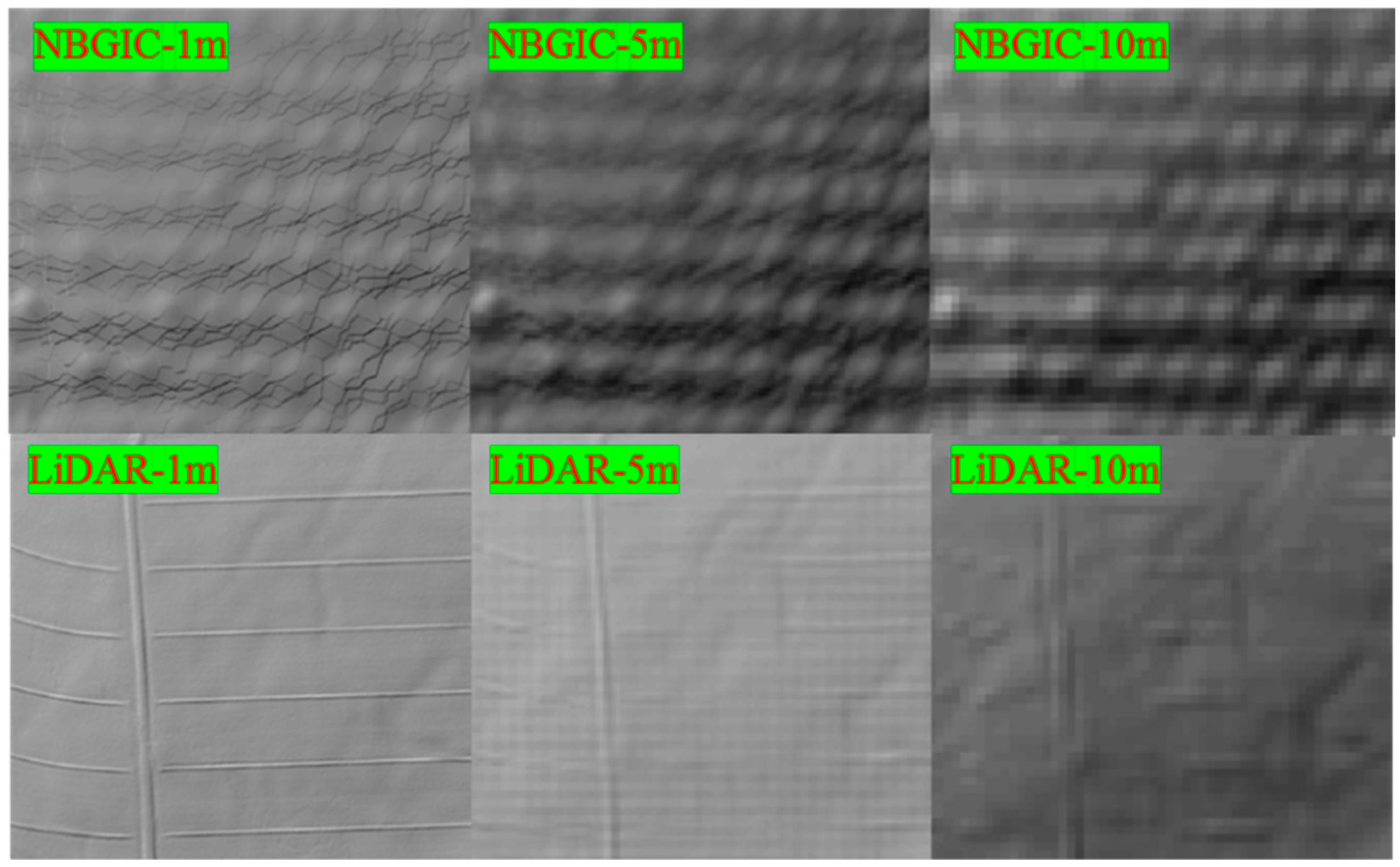
Figure 4 shows the hillshade of different resolution and accuracy DEMs for a patch of terrace in BBW (Figure 1). Apparently, LiDAR DEMs were better than NBGIC DEMs in depicting micro features. Especially, LiDAR-1m DEM could reveal detailed topography in FDT systems.

4.1. Slope Calculation with ANS and DHS for Different DEMs

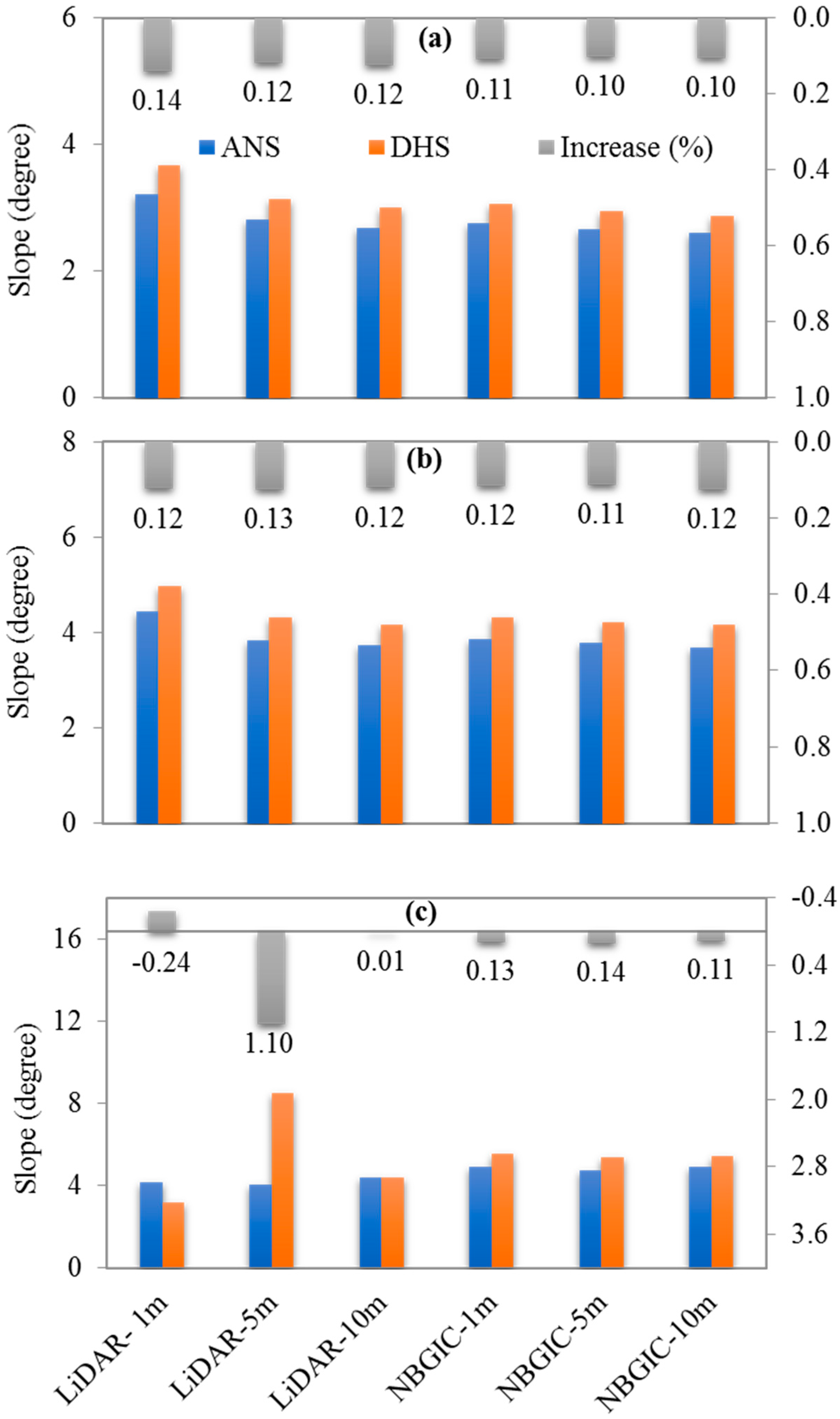
The mean slopes for the whole watershed, a terrace patch, and 1 m-buffer zones in front of embankments (i.e., greased flow channels) within the patch from different DEMs using ANS and HDS methods are shown in

Table 1. Slope (degree) calculated with six DEMs using the DHS and ANS method for watershed, terrace patch, and buffer areas.

		LiDAR-1m	LiDAR-5m	LiDAR-10m	NBGIC-1m	NBGIC-5m	NBGIC-10m
Basin	ANS	3.22	2.81	2.68	2.76	2.67	2.60
	DHS	3.67	3.14	3.01	3.06	2.94	2.87
Terrace	ANS	4.43	3.82	3.72	3.86	3.78	3.69
	DHS	4.98	4.30	4.17	4.31	4.21	4.15
Buffer	ANS	4.16	4.05	4.36	4.89	4.72	4.88
	DHS	3.18	8.52	4.41	5.52	5.37	5.41

and Figure 5. All the mean slopes derived from the DHS method were greater than those derived from ANS method for the whole watershed and terrace patch with different DEMs (Figure 5a,b). For the whole watershed, the DHS method increased the mean slopes by 10–14% compared to those derived from the ANS method, while for the terrace patch, the DHS method increased the mean slopes by 11–13% (Figure 5a,b). The results indicated that the DHS method tended to increase slopes for large and relatively flat areas regardless of the resolution and accuracy of DEMs. This is also true for NBGIC DEMs in the 1 m-buffer zones (Figure 5c) at three different solutions mainly due to their low accuracy.

However, the mean slope derived from the DHS method (3.18°) was smaller than that derived from the ANS method (4.16°) for LiDAR-1m DEM (Table 1; Figure 5c). This result indicated that with LiDAR-1m, DHS method can better account for the actual slope in front of embankments where sediment deposition occurred. In contrast, the mean slopes derived from the DHS method were greater that those derived by the ANS method for LiDAR-5 and 10 m DEMs (Table 1; Figure 5c). Notice that the mean slope derived from the DHS method (8.52°) was more than twice greater than the mean slope derived from the ANS method (4.04°) for LiDAR-5m DEM (Table 1; Figure 5c). This is because the size of embankments and grassed flow channels were close to but smaller than the resolution of LiDAR-5m DEM. Consequently, the large vertical distances between high points on embankments and low points around the embankments misled the flow direction when the DHS method was used. For the LiDAR-10 m DEM, the difference between two slope-calculation methods was insignificant indicating that DHS exhibited its advantage alculated with six DEMs using the DHS and ANS method for watershed, terrace patch, and buffer area.

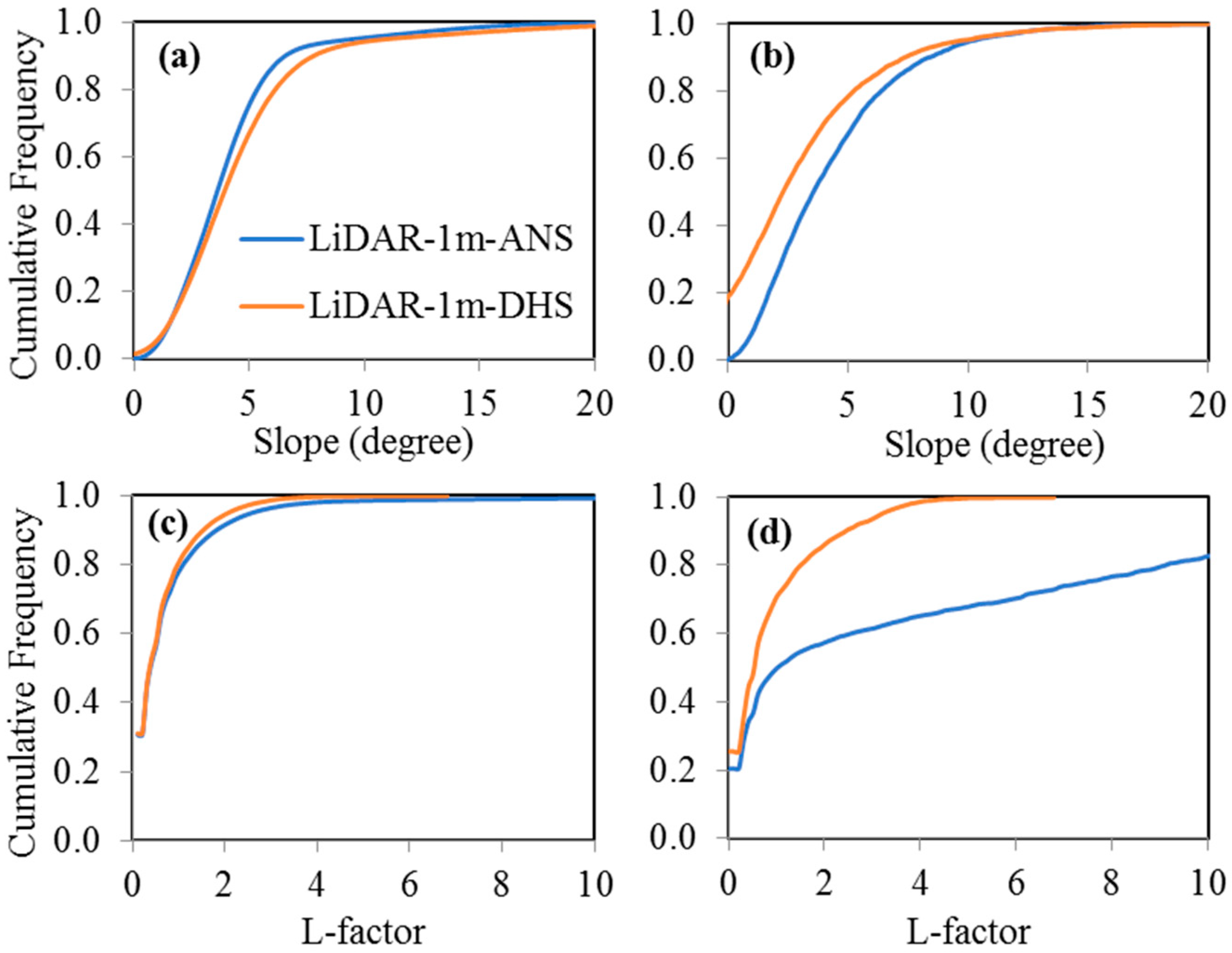
Cumulative frequency curves for calculated slopes in the terrace patch and grassed flow channels derived from LiDAR-1m DEM are shown in Figure 6a,b, respectively. The DHS method produced greater slopes than the ANS method in the terrace patch (Figure 6a). For the grassed flow channels, however, the slopes calculated by DHS method were distinctively smaller than those derived from the ANS method (Figure 6b). Figure 6b showed that near 20% of slopes were equal to zero in grassed flow channels calculated by the DHS method. In contrast, the ANS method could not detect those flat areas. This result further proved that the DHS method was feasible for slope calculation in FDT systems.

Based on above analysis, slopes calculated by the DHS method were greater than those derived from the ANS method in segments between embankments, while calculated slopes in front of embankments were smaller for the DHS method than those calculated by the ANS method when the LiDAR-1m DEM was used. Compared with the ANS method, the DHS method has the capacity of reflecting the real world topographical features when high resolution and accuracy DEMs were used. However, if coarser resolution or less accurate DEMs were used in calculating slope, the DHS method tended to produce greater slopes than those generated by the ANS method. Therefore, it is recommended that the DHS method should be used to calculate slopes in FDT systems when high resolution and accuracy DEMs are used.

4.2. The L-Factor Determined by ANS and DHS for LiDAR-1m DEM

The L-factor derived from LiDAR-1m DEM was calculated by setting slope cut-off value at 0.99 for the DHS and ANS methods in the terrace patch and 1 m-buffer zones. Statistical summary of calculated L-factor values is shown in

Table 2. Statistical summary of L-factor values calculated by the DHS and ANS methods with LiDAR-1m DEM for terrace patch and buffer areas.

		Min	Max	Mean
Terrace	ANS	0	18.16	0.76
	DHS	0	6.08	0.59
Buffer	ANS	0	18.16	4.12
	DHS	0	6.73	0.87

. Both maximal and mean values of L-factor calculated by the ANS method were greater than those calculated by the DHS method in the terrace patch and 1 m-buffer zones. However, the difference between mean L-factors calculated by the ANS and DHS methods for 1 m-buffer zones was 3.25, much greater than that for the terrace patch (i.e., 0.17). This result indicated that L-factor calculated by the DHS method was more sensitive to topographical variations than that calculate by the ANS method, i.e., the DHS method tended to account for soil deposition areas in FDT systems.

The cumulative frequency of L-factor values is showed in Figure 6c,d in the terrace patch and grassed flow channels, respectively. The range of L-factor values calculated by the DHS method were smaller than those derived from the ANS method for the terrace patch and buffer areas. At the same time, L-factor values calculated by the DHS method were smaller than those calculated by the ANS method for both areas with greater differences occurred in buffer areas. We can conclude that the ANS method cannot detect sediment deposition areas which potentially result in overestimation of soil losses in terrace areas especially in areas in front of embankments.

4.3. Soil Loss Calculation with ANS and DHS for Different DEMs

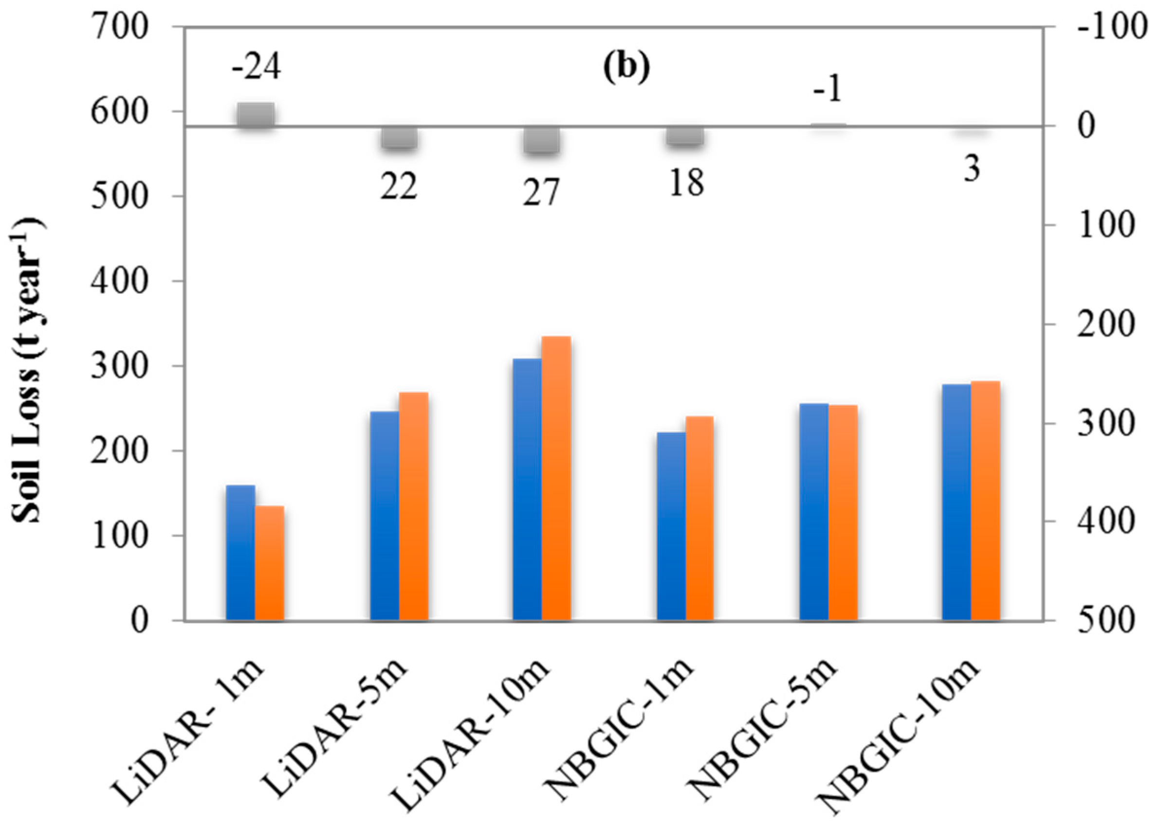
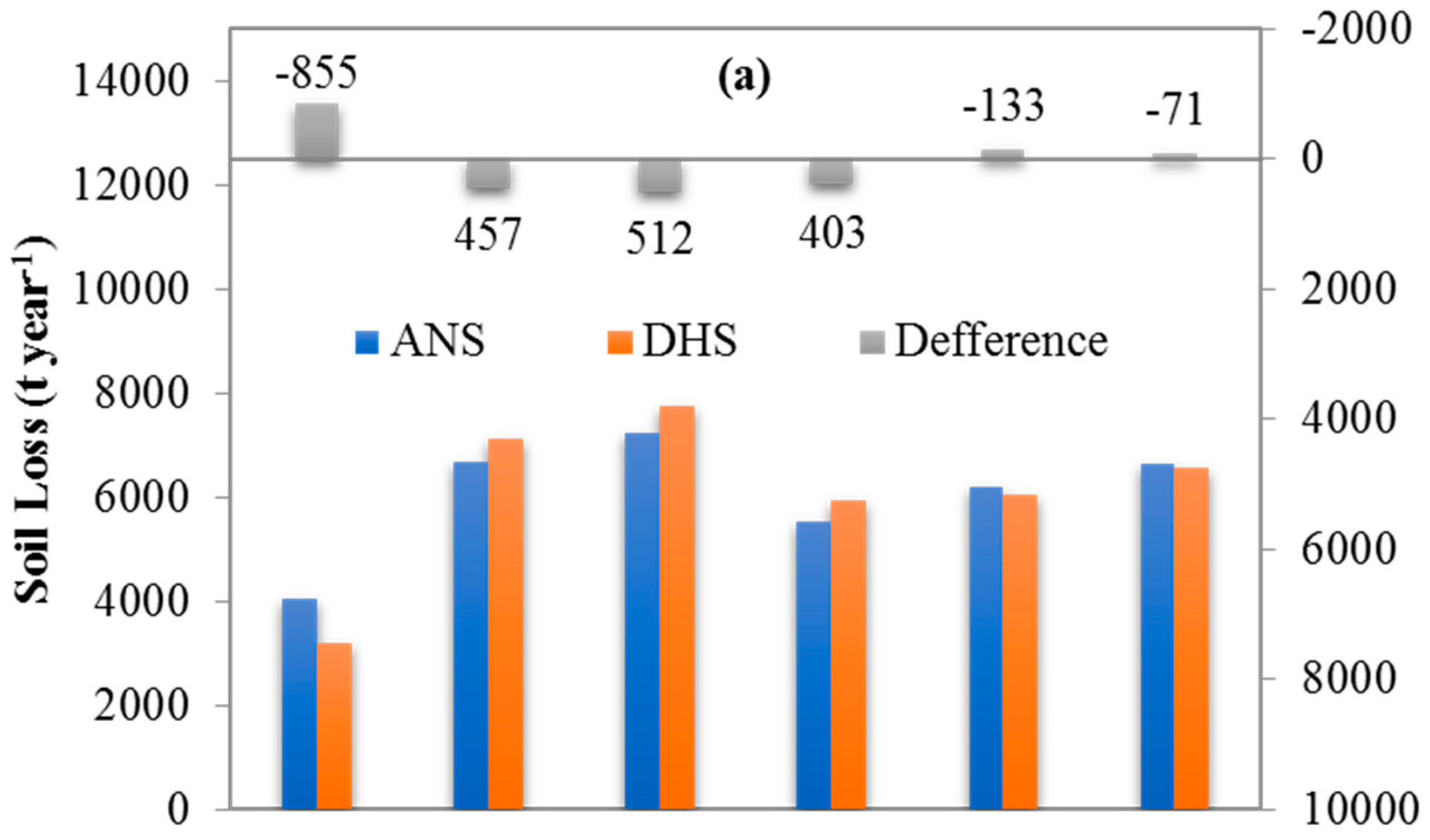
Predicted annual soil losses for the whole watershed and terrace patch in 2000 are shown in

Table 3. Soil losses calculated by the DHS and ANS methods with six DEMs for the whole watershed and a terrace patch.

		LiDAR-1m	LiDAR-5m	LiDAR-10m	NBGIC-1m	NBGIC-5m	NBGIC-10m
Basin	ANS	4048	6658	7224	5515	6191	6628
	DHS	3193	7115	7736	5918	6058	6557
Terrace	ANS	159	247	309	223	256	279
	DHS	135	269	336	241	255	282

. Soil losses calculated with the DHS method were greater than or approximate with those predicted with the ANS method for respective NBGIC and LiDAR DEMs, except that soil loss from LiDAR-1m DEM with the DHS method was distinctly smaller than that predicted with the ANS method (Figure 7a). It is worth noting that the predicted annual soil loss for BBW from LiDAR-1m DEM with DHS method was very close to the measurement (3193 vs. 3211 t year⁻¹). This result showed that P-factor is not needed for assessment of soil conservation effect of FDT systems using high resolution and accuracy DEMs with accurate estimates of LS-factor, which is accounting for physical causes for soil loss reduction of FDT. For the terrace patch, soil losses calculated with the DHS method were greater than or approximate with those predicted with the ANS method for respective NBGIC and LiDAR DEMs, except that soil losses predicted from LiDAR-1m DEM with the DHS method was distinctly smaller than those predicted with the ANS method (Figure 7b).

Interestingly, the DHS method generated greater mean slopes and smaller mean L-factor values for the whole watershed and terrace patch than those calculated by the ANS method, whereas predicted soil losses with the DHS method were less than those predicted with the ANS method. This indicated that L-factor had a greater impact on soil loss estimation than S-factor with other factors keeping constant. With high resolution and accuracy DEMs, the DHS method is needed to calculate topographical features such as S-factor and L-factor as inputs in soil erosion models like RUSLE. This method would improve the assessment of FDT on soil conservation in watersheds.

5. Conclusions

Slope is an important topographical parameter influencing hydrological processes on the land surface. In flow diversion terrace (FDT) systems, great changes in slope are produced due to micro variations of topography. As a result, assessing the effectiveness of FDT on soil conservation has different results with different slope calculation methods. With the emergence of high resolution and accuracy digital elevation models (DEMs) from light detection and ranging (LiDAR) data, the suitability of existing algorithms in calculating slope for hydrological applications needs to be reassessed. In this study, the ArcGIS built-in average-neighborhood-slope (ANS) method and a downhill-slope (DHS) method were used to calculate slopes in a small agricultural watershed, New Brunswick, Canada. Six DEMs were used to evaluate those two methods, i.e., 1, 5 and 10 m resolution DEMs interpolated from irregular height point-data generated with conventional photogrammetric techniques, and 1, 5, and 10 m resolution DEMs derived from LiDAR data. Calculated slopes were summarized for the entire watershed, a patch of terrace, and grassed flow channels in front of embankments. Results indicated that the DHS method produced smaller slopes than the ANS method with LiDAR-1m DEM along grasses flow channels. In addition, slope-dependent L-factor was calculated based on the ANS and DHS methods in the terrace patch and grassed flow channels with LiDAR-1m DEM. Results showed that the mean value of L-factor derived from the DHS was smaller than that derived from the ANS method in both areas with the greatest difference occurring in front of embankments. Finally, the revised universal soil loss equation (RUSLE) was used to estimate soil losses at the watershed and terrace patch using the ANS and DHS methods. Soil losses estimated from the DHS method were smaller than those derived from the ANS method for those two areas with the LiDAR-1m DEM. In addition, the soil loss estimated by the DHS method was more consistent with measurement in the watershed. We concluded that the DHS method is suitable in calculating slopes along grassed flow channels and can be used to estimate slope with high resolution and accuracy LiDAR-based DEMs. The DHS method can accurately estimate topographical features such as S-factor and L-factor in USLE-based models and, as a result, can improve the assessment of FDT systems in watersheds. In addition, we also demonstrated that soil loss can be estimated for FDT systems by correct calculation of LS-factor without altering P-factor when high resolution and accuracy DEMs were used. DHS method has the potential to be used with SWAT application when high resolution and accuracy DEMs are available.

References

- Chow, T.; Rees, H.; Daigle, J. Effectiveness of terraces/grassed waterway systems for soil and water conservation: A field evaluation. J. Soil Water Conserv. 1999, 54, 577–583. [Google Scholar]
- Yang, Q.; Meng, F.-R.; Zhao, Z.; Chow, T.L.; Benoy, G.; Rees, H.W.; Bourque, C.P.-A. Assessing the impacts of flow diversion terraces on stream water and sediment yields at a watershed level using swat model. Agric. Ecosyst. Environ. 2009, 132, 23–31. [Google Scholar] [CrossRef]
- Yang, Q.; Zhao, Z.; Benoy, G.; Chow, T.L.; Rees, H.W.; Bourque, C.P.-A.; Meng, F.-R. A watershed-scale assessment of cost-effectiveness of sediment abatement with flow diversion terraces. J. Environ. Qual. 2010, 39, 220–227. [Google Scholar] [CrossRef] [PubMed]
- Arnold, J.G.; Srinivasan, R.; Muttiah, R.S.; Williams, J.R. Large area hydrologic modeling and assessment part I: Model development. JAWRA J. Am. Water Resour. Assoc. 1998, 34, 73–89. [Google Scholar] [CrossRef]
- Haan, C.T.; Barfield, B.J.; Hayes, J.C. Design Hydrology and Sedimentology for Small Catchments; Academic Press: San Diego, CA, USA, 1994. [Google Scholar]
- Morgan, R.P.C.; Nearing, M. Handbook of Erosion Modelling; John Wiley & Sons: New York, NY, USA, 2016. [Google Scholar]
- Panagos, P.; Borrelli, P.; Meusburger, K.; van der Zanden, E.H.; Poesen, J.; Alewell, C. Modelling the effect of support practices (p-factor) on the reduction of soil erosion by water at European scale. Environ. Sci. Policy 2015, 51, 23–34. [Google Scholar] [CrossRef] [Green Version]
- Wischmeier, W.H.; Smith, D.D. Predicting Rainfall Erosion Losses—A Guide to Conservation Planning; Agriculture Handbook No. 537; U.S. Department of Agriculture: Washington, DC, USA, 1978.
- Mitasova, H.; Hofierka, J.; Zlocha, M.; Iverson, L.R. Modelling topographic potential for erosion and deposition using GIS. Int. J. Geogr. Inf. Syst. 1996, 10, 629–641. [Google Scholar] [CrossRef] [Green Version]
- Hickey, R. Slope angle and slope length solutions for GIS. Cartography 2000, 29, 1–8. [Google Scholar] [CrossRef]
- Mitas, L.; Mitasova, H. Distributed soil erosion simulation for effective erosion prevention. Water Resour. Res. 1998, 34, 505–516. [Google Scholar] [CrossRef] [Green Version]
- Burrough, P.A.; McDonnell, R.A. Principles of GIS; Oxford University Press: London, UK, 1998. [Google Scholar]
- Yang, Q.; Zhao, Z.; Chow, T.L.; Rees, H.W.; Bourque, C.P.A.; Meng, F.R. Using GIS and a digital elevation model to assess the effectiveness of variable grade flow diversion terraces in reducing soil erosion in northwestern New Brunswick, Canada. Hydrol. Process. 2009, 23, 3271–3280. [Google Scholar] [CrossRef]
- Moore, I.D.; Burch, G.J. Physical basis of the length-slope factor in the universal soil loss equation. Soil Sci. Soc. Am. J. 1986, 50, 1294–1298. [Google Scholar] [CrossRef]
- Panuska, J.C.; Moore, I.D.; Kramer, L.A. Terrain analysis: Integration into the agricultural nonpoint source (AGNPS) pollution model. J. Soil Water Conserv. 1991, 46, 59–64. [Google Scholar]
- Desmet, P.; Govers, G. A GIS procedure for automatically calculating the USLE LS factor on topographically complex landscape units. J. Soil Water Conserv. 1996, 51, 427–433. [Google Scholar]
- Foster, G.; Wischmeier, W. Evaluating irregular slopes for soil loss prediction. Trans. ASAE 1974, 17, 0305–0309. [Google Scholar] [CrossRef]
- Zhao, Z.; Benoy, G.; Chow, T.L.; Rees, H.W.; Daigle, J.-L.; Meng, F.-R. Impacts of accuracy and resolution of conventional and lidar based DEMs on parameters used in hydrologic modeling. Water Resour. Manag. 2010, 24, 1363–1380. [Google Scholar] [CrossRef]
- Li, Q.; Qi, J.; Xing, Z.; Li, S.; Jiang, Y.; Danielescu, S.; Zhu, H.; Wei, X.; Meng, F.-R. An approach for assessing impact of land use and biophysical conditions across landscape on recharge rate and nitrogen loading of groundwater. Agric. Ecosyst. Environ. 2014, 196, 114–124. [Google Scholar] [CrossRef]
- Chow, T.; Rees, H. Impacts of Intensive Potato Production on Water Yield and Sediment Load (Black Brook Experimental Watershed: 1992–2002 Summary); Potato Research Centre, AAFC: Fredericton, NB, Canada, 2006; p. 26.
- Qi, J.; Li, S.; Li, Q.; Xing, Z.; Bourque, C.P.-A.; Meng, F.-R. Assessing an enhanced version of swat on water quantity and quality simulation in regions with seasonal snow cover. Water Resour. Manag. 2016, 30, 5021–5037. [Google Scholar] [CrossRef]
- Qi, J.; Li, S.; Jamieson, R.; Hebb, D.; Xing, Z.; Meng, F.-R. Modifying swat with an energy balance module to simulate snowmelt for maritime regions. Environ. Model. Softw. 2017, 93, 146–160. [Google Scholar] [CrossRef]
- Mellerowicz, K.T. Soils of the Black Brook Watershed St. Andre Parish, Madawaska County, New Brunswick; New Brunswick Department of Agriculture: Fredericton, NB, Canada, 1993.
- Qi, J.; Li, S.; Yang, Q.; Xing, Z.; Meng, F.-R. Swat setup with long-term detailed landuse and management records and modification for a micro-watershed influenced by freeze-thaw cycles. Water Resour. Manag. 2017, 31, 3953–3974. [Google Scholar] [CrossRef]
- Zhao, Z.; Chow, T.L.; Yang, Q.; Rees, H.W.; Benoy, G.; Xing, Z.; Meng, F.-R. Model prediction of soil drainage classes based on digital elevation model parameters and soil attributes from coarse resolution soil maps. Can. J. Soil Sci. 2008, 88, 787–799. [Google Scholar] [CrossRef] [Green Version]
- Qi, J.; Li, S.; Li, Q.; Xing, Z.; Bourque, C.P.-A.; Meng, F.-R. A new soil-temperature module for swat application in regions with seasonal snow cover. J. Hydrol. 2016, 538, 863–877. [Google Scholar] [CrossRef]
- Wall, G.; Coote, D.; Pringle, E.; Shelton, I. Revised Universal Soil Loss Equation for Application in Canada: A Handbook for Estimating Soil Loss from Water Erosion in Canada; Contribution No. AAFCAAC2244E; Agriculture and Agri-Food Canada, Research Branch: Ottawa, ON, Canada, 2002.
- Moore, I.D.; Wilson, J.P. Length-slope factors for the revised universal soil loss equation: Simplified method of estimation. J. Soil Water Conserv. 1992, 47, 423–428. [Google Scholar]
- Ashraf, M.I.; Zhao, Z.; Bourque, C.P.A.; Meng, F.R. GIS-evaluation of two slope-calculation methods regarding their suitability in slope analysis using high-precision lidar digital elevation models. Hydrol. Process. 2012, 26, 1119–1133. [Google Scholar] [CrossRef]
- Hill, A.J.; Neary, V.S. Factors affecting estimates of average watershed slope. J. Hydrol. Eng. 2005, 10, 133–140. [Google Scholar] [CrossRef]
- Fernandez, C.; Wu, J.; McCool, D.; Stöckle, C. Estimating water erosion and sediment yield with GIS, RUSLE, and SEDD. J. Soil Water Conserv. 2003, 58, 128–136. [Google Scholar]
© 2018 by the authors. Licensee MDPI, Basel, Switzerland. This article is an open access article distributed under the terms and conditions of the Creative Commons Attribution (CC BY) license (http://creativecommons.org/licenses/by/4.0/).