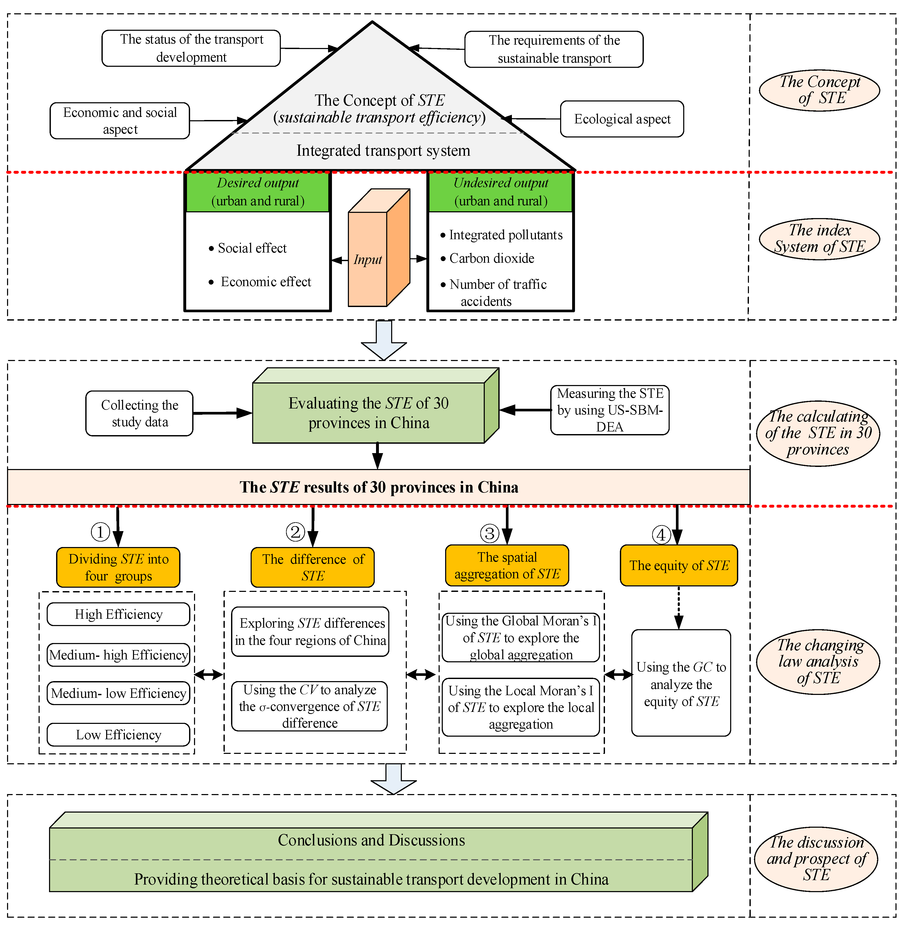
Figure 1.
The research framework.
Figure 1.
The research framework.
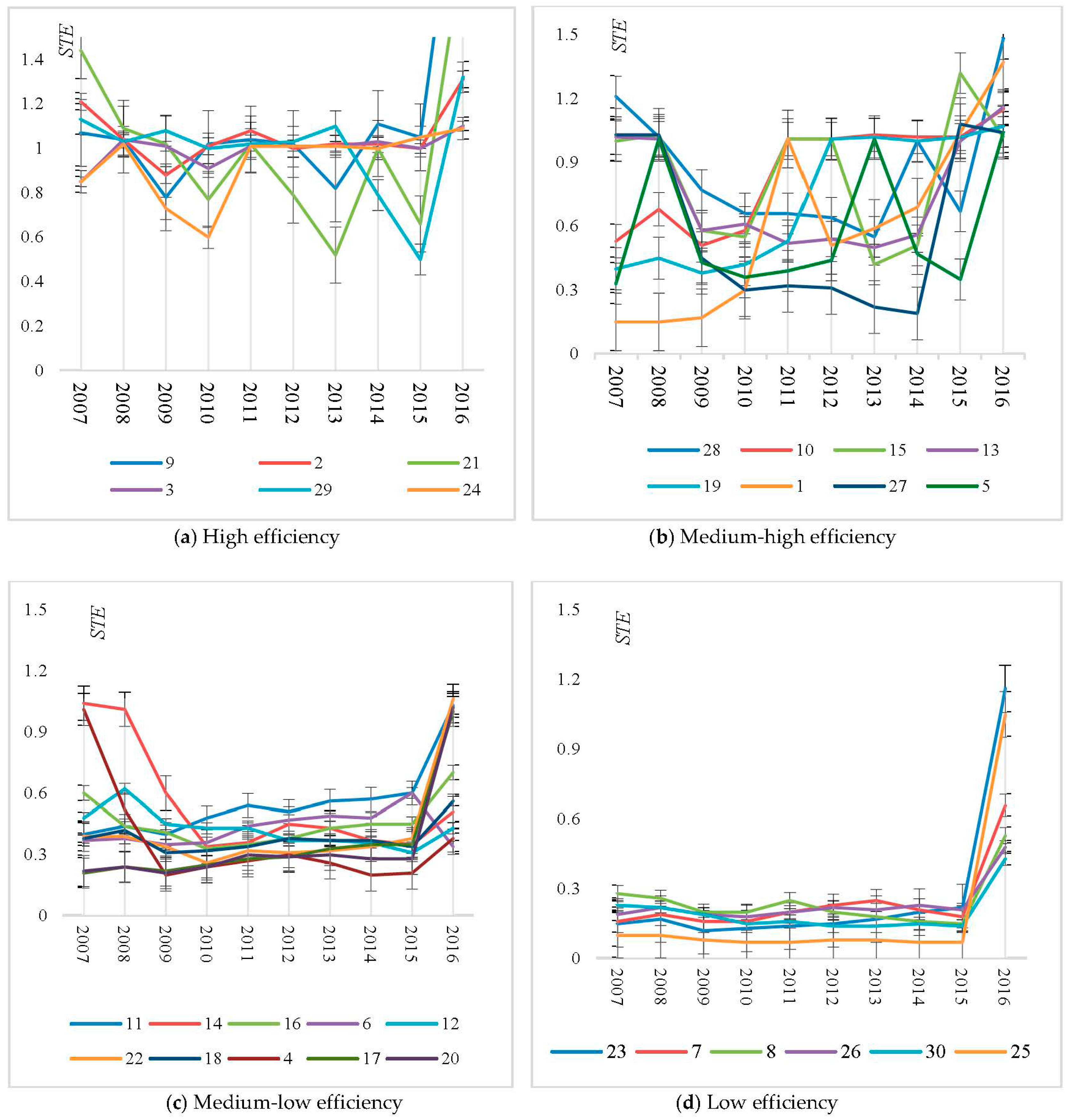
Figure 2.
Changing trend of four groups of STE from 2007 to 2016. Note: Province no. 1. Beijing, 2. Tianjin, 3. Hebei, 4. Shanxi, 5. Inner Mongolia, 6. Liaoning, 7. Jilin, 8. Heilongjiang, 9. Shanghai, 10. Jiangsu, 11. Zhejiang, 12. Anhui, 13. Fujian, 14. Jiangxi, 15. Shandong, 16. Henan, 17. Hubei, 18. Hunan, 19. Guangdong, 20. Guangxi, 21. Hainan, 22. Chongqing, 23. Sichuan, 24. Guizhou, 25. Yunnan, 26. Shaanxi, 27. Gansu, 28. Ningxia, 29. Qinghai, 30. Xinjiang.
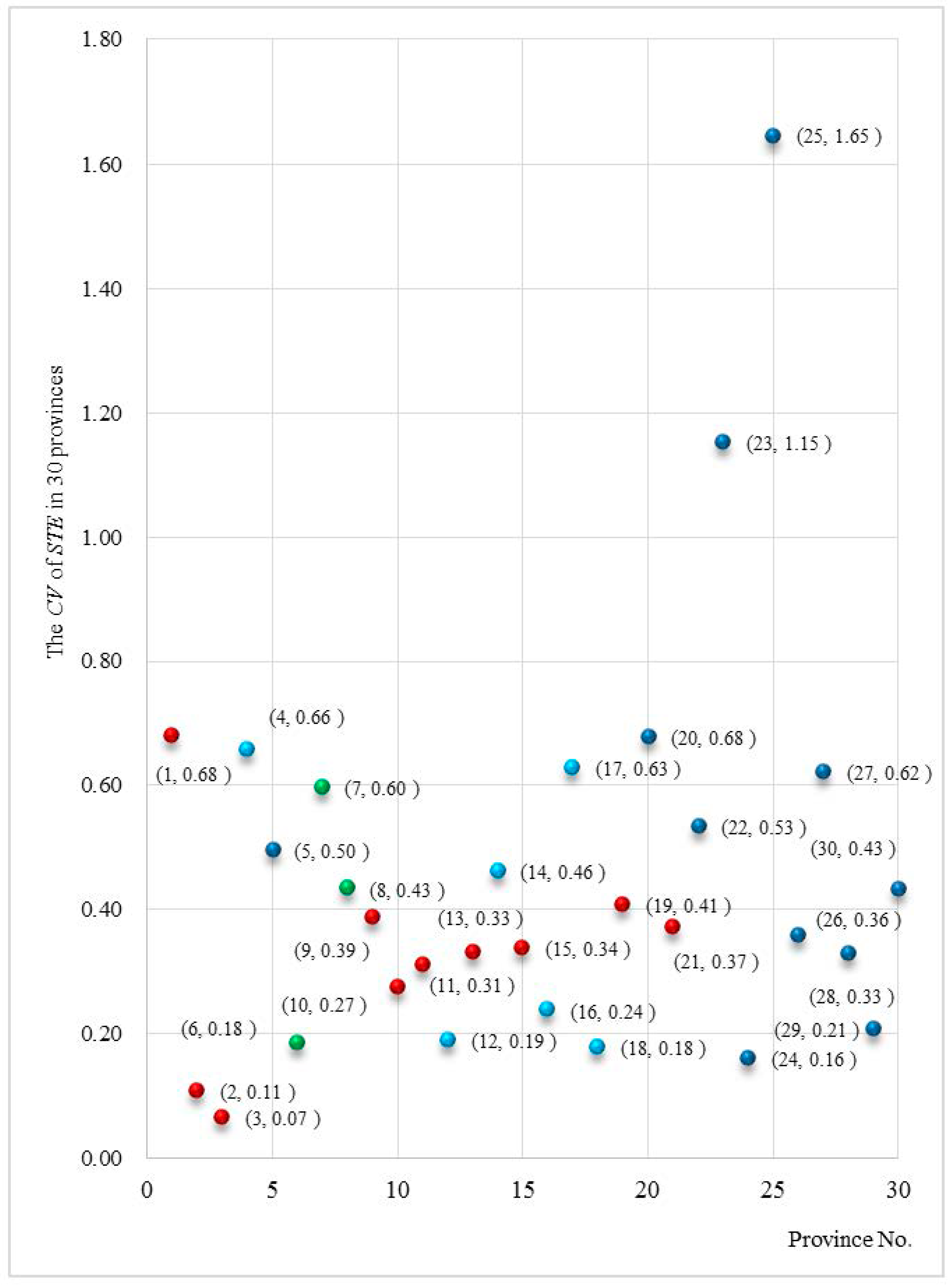
Figure 3.
STE difference results of 30 provinces. Note: (number, number) represents (province no., CV). Province no. 1. Beijing, 2. Tianjin, 3. Hebei, 4. Shanxi, 5. Inner Mongolia, 6. Liaoning, 7. Jilin, 8. Heilongjiang, 9. Shanghai, 10. Jiangsu, 11. Zhejiang, 12. Anhui, 13. Fujian, 14. Jiangxi, 15. Shandong, 16. Henan, 17. Hubei, 18. Hunan, 19. Guangdong, 20. Guangxi, 21. Hainan, 22. Chongqing, 23. Sichuan, 24.Guizhou, 25. Yunnan, 26. Shaanxi, 27. Gansu, 28. Ningxia, 29. Qinghai, 30. Xinjiang.
![Sustainability 10 02399 i001]()
represent the eastern, central, western, and northeast regions, respectively.
Figure 4.
Four regional divisions of mainland China. Note: Province no. 1. Beijing, 2. Tianjin, 3. Hebei, 4. Shanxi, 5. Inner Mongolia, 6. Liaoning, 7. Jilin, 8. Heilongjiang, 9. Shanghai, 10. Jiangsu, 11. Zhejiang, 12. Anhui, 13. Fujian, 14. Jiangxi, 15. Shandong, 16. Henan, 17. Hubei, 18. Hunan, 19. Guangdong, 20. Guangxi, 21. Hainan, 22. Chongqing, 23. Sichuan, 24.Guizhou, 25. Yunnan, 26. Shaanxi, 27. Gansu, 28. Ningxia, 29. Qinghai, 30. Xinjiang.
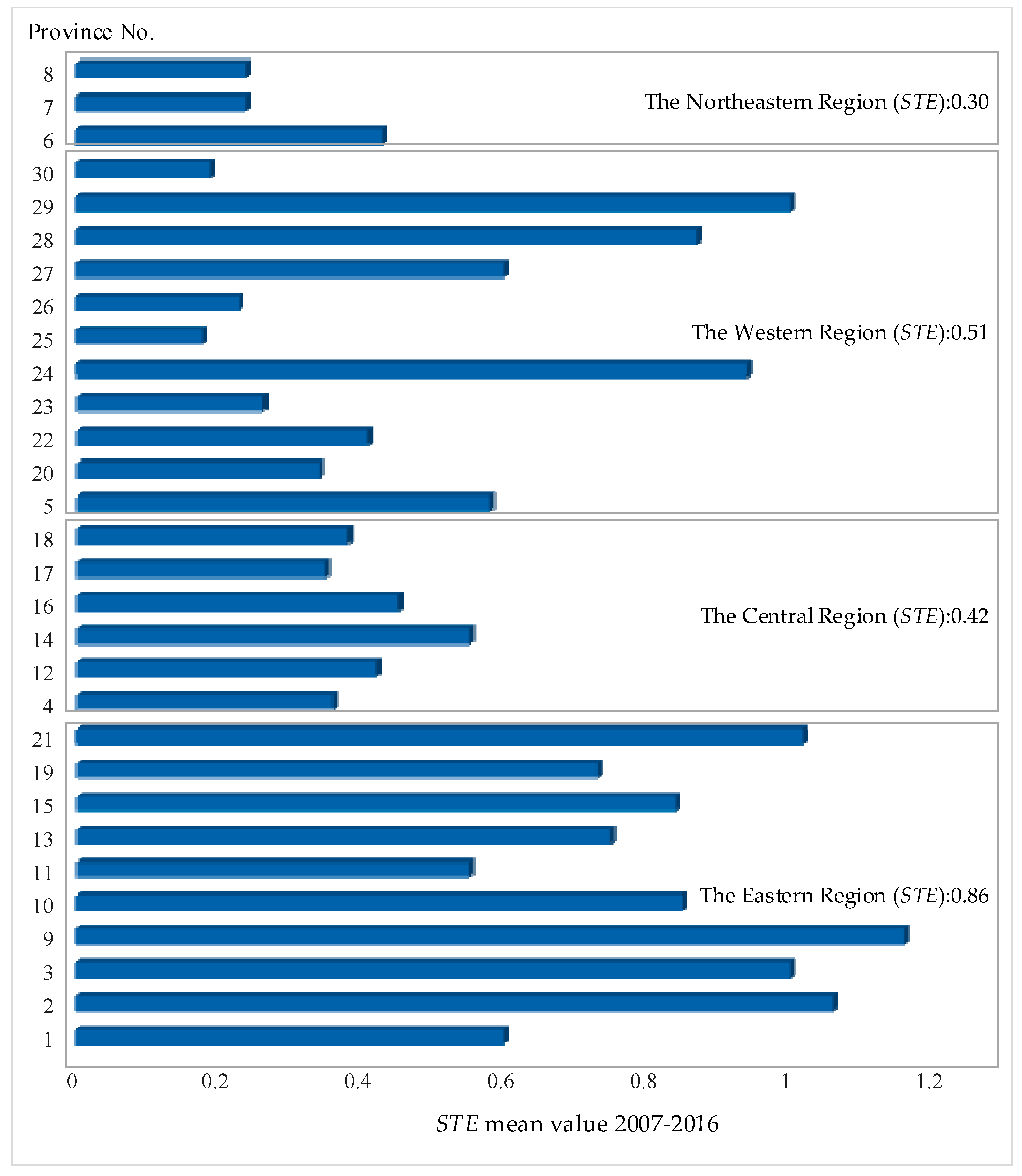
Figure 5.
Overall STE in China. Note: Province no. 1. Beijing, 2. Tianjin, 3. Hebei, 4. Shanxi, 5. Inner Mongolia, 6. Liaoning, 7. Jilin, 8. Heilongjiang, 9. Shanghai, 10. Jiangsu, 11. Zhejiang, 12. Anhui, 13. Fujian, 14. Jiangxi, 15. Shandong, 16. Henan, 17. Hubei, 18. Hunan, 19. Guangdong, 20. Guangxi, 21. Hainan, 22. Chongqing, 23. Sichuan, 24.Guizhou, 25. Yunnan, 26. Shaanxi, 27. Gansu, 28. Ningxia, 29. Qinghai, 30. Xinjiang.
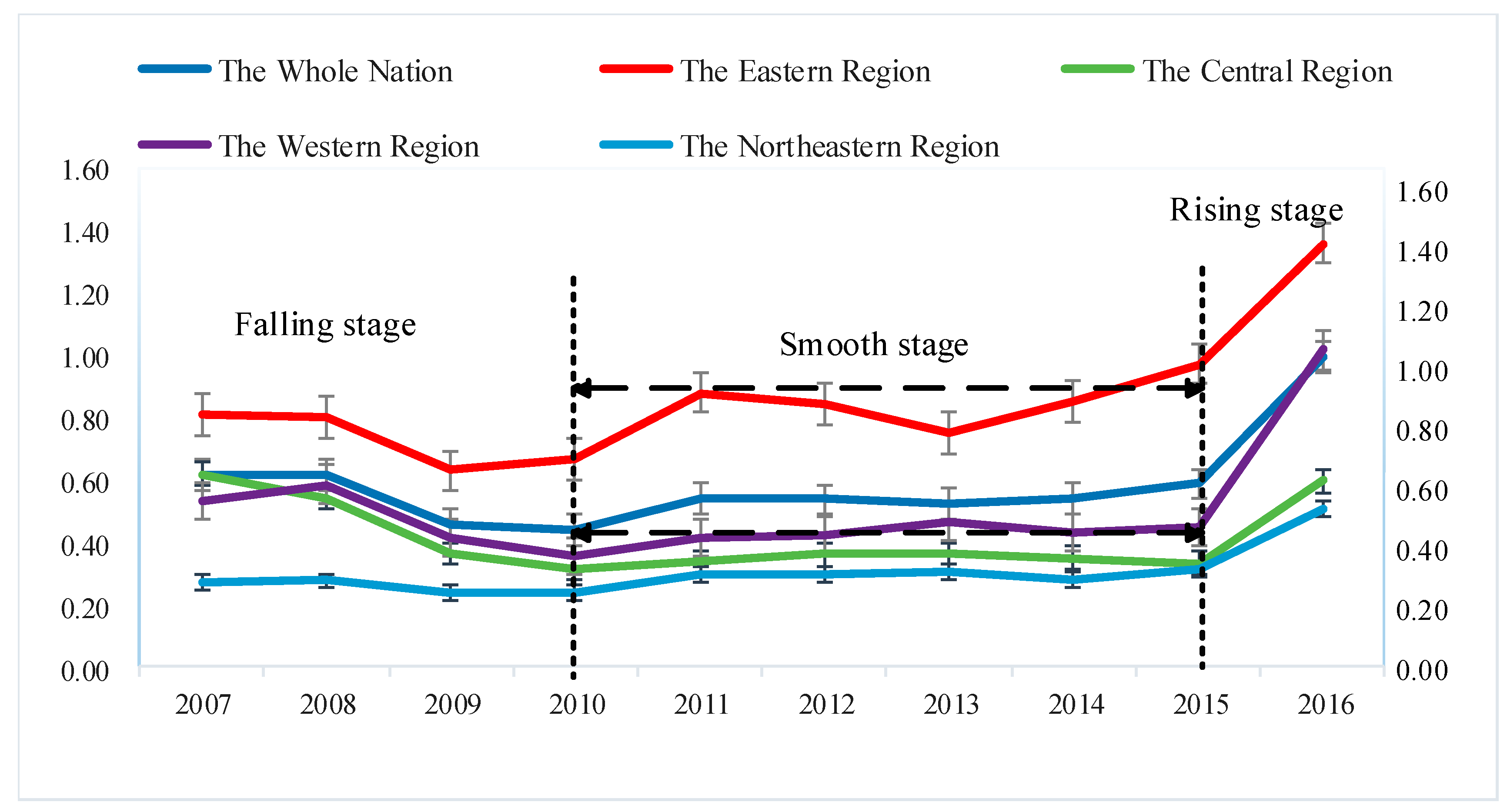
Figure 6.
The trend of STE in four regions in China from 2007 to 2016.
Figure 6.
The trend of STE in four regions in China from 2007 to 2016.
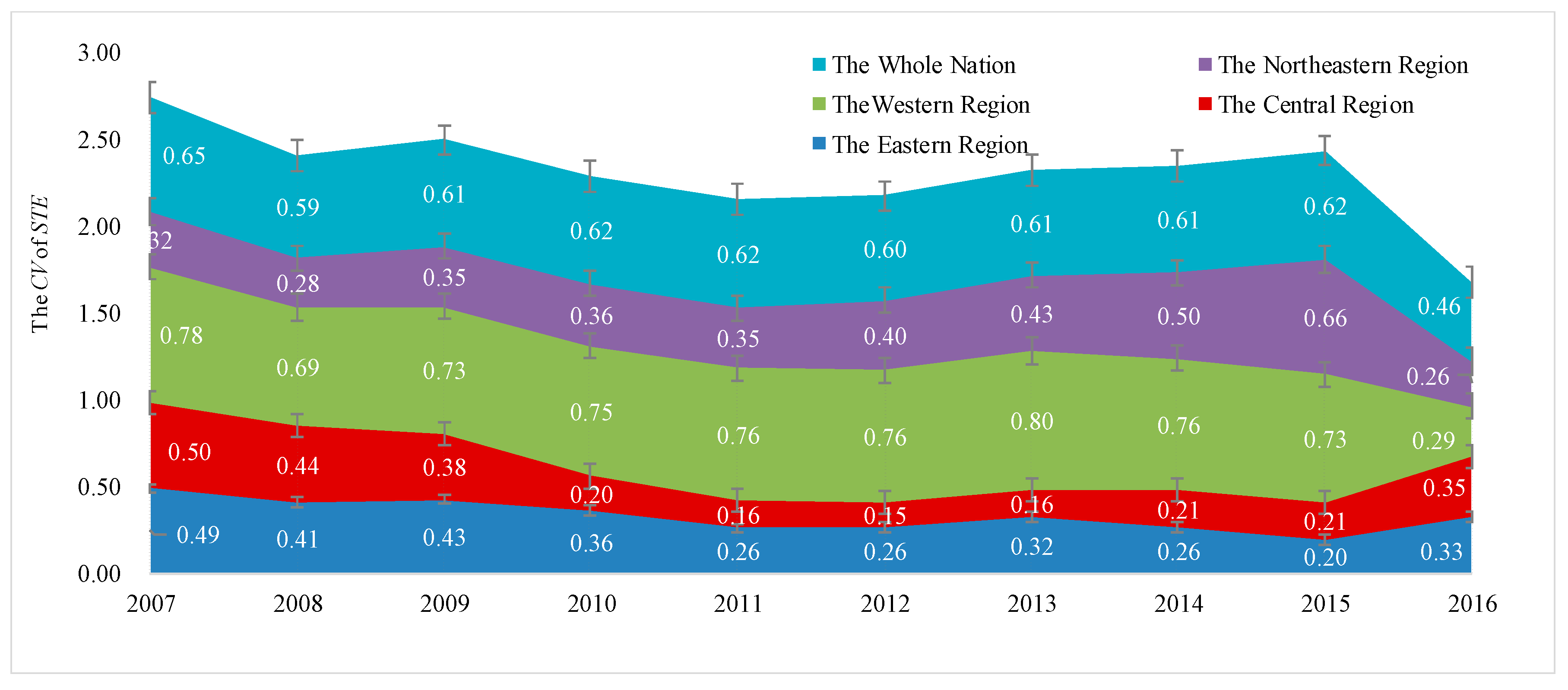
Figure 7.
Changes in STE difference of the four regions from 2007 to 2016.
Figure 7.
Changes in STE difference of the four regions from 2007 to 2016.
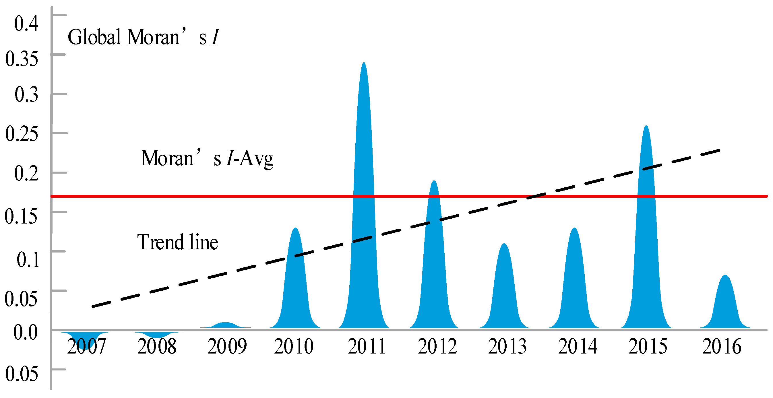
Figure 8.
Global Moran’s I, 2007–2016.
Figure 8.
Global Moran’s I, 2007–2016.
Figure 9.
Moran scatter plot of STE. Note: Province no. 1. Beijing, 2. Tianjin, 3. Hebei, 4. Shanxi, 5. Inner Mongolia, 6. Liaoning, 7. Jilin, 8. Heilongjiang, 9. Shanghai, 10. Jiangsu, 11. Zhejiang, 12. Anhui, 13. Fujian, 14. Jiangxi, 15. Shandong, 16. Henan, 17. Hubei, 18. Hunan, 19. Guangdong, 20. Guangxi, 21. Hainan, 22. Chongqing, 23. Sichuan, 24.Guizhou, 25. Yunnan, 26. Shaanxi, 27. Gansu, 28. Ningxia, 29. Qinghai, 30. Xinjiang.
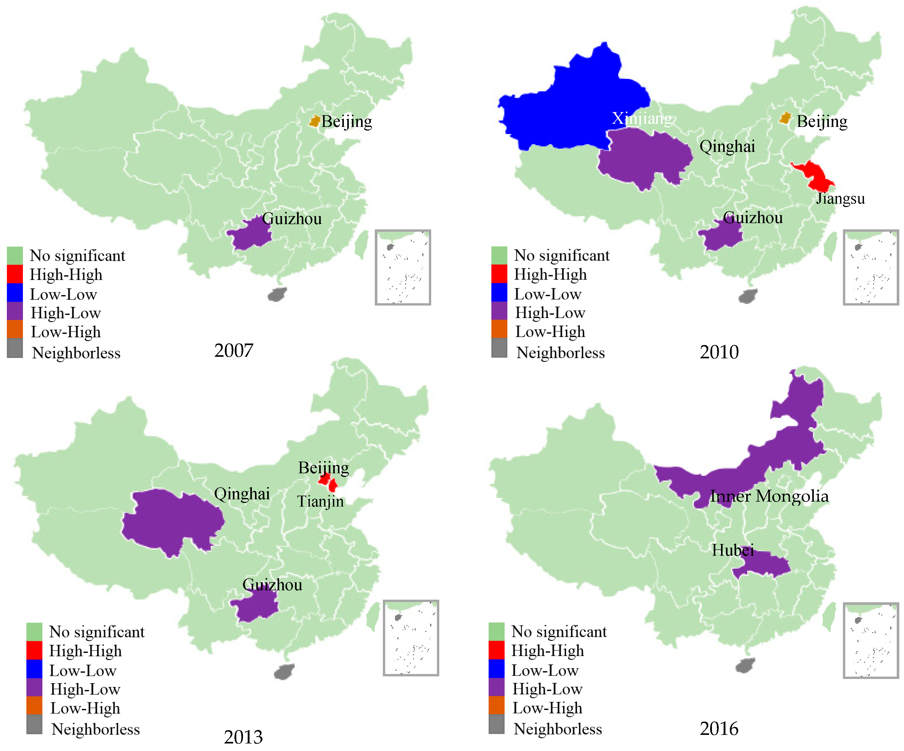
Figure 10.
LISA map of STE.
Figure 10.
LISA map of STE.
Table 1.
Literature on transport efficiency evaluation.
Table 1.
Literature on transport efficiency evaluation.
| Authors | Year | Inputs | Outputs |
|---|
| Woo et al. [48] | 2015 | Labor, capital, energy | Added value, carbon emissions, power generation |
| Cui et al. [49] | 2014 | Employees and consumption | CO2 emissions and added value |
| X. Guo et al. [50] | 2017 | Coal and electricity consumption | Gross domestic product |
| Z. Wei et al. [51] | 2012 | Energy, capital investment | Intelligent traffic management benefits |
| L. Yang et al. [52] | 2015 | Labor, capital, resources | Gross domestic product |
| Sami Jet al. [27] | 2013 | Operating expenses, number of employees | Benefits |
| Xin Xu et al. [53] | 2017 | Number of employees, capital investment, aviation consumption | Added value |
| Duygun et al. [54] | 2016 | Capital, employees, materials | Income |
Table 2.
Summary of input and output variables.
Table 2.
Summary of input and output variables.
| Criteria Layer | Element Layer | Indicator Variable | Metric |
|---|
| Input indicators | Production factor input | Transport investment in fixed assets (TIFA) | 108 yuan |
| Private car ownership (PCO) | 104 vehicles |
| Length of transport line (LTL) | 104 kms |
| Energy factor input | Transport energy consumption (TEC) | Tons of standard coal |
| Labor factor input | Transport practitioners (TP) | Person |
| Land factor input | Land use of transport (LUT) | 103 hectares |
| Desired output indicators | Social effect output | Passenger and freight turnover (PFT) | 108 tons km |
| Economic effect output | Added value of transport sector (AVT) | 108 yuan |
| Undesired output indicators | Negative effect output | Integrated pollutants emissions (IPE) | Kilogram |
| Carbon dioxide (CD) | Ton |
| Number of traffic accidents (NTC) | Case |
Table 3.
Conversion factor for passenger and freight turnover.
Table 3.
Conversion factor for passenger and freight turnover.
| Conversion Factor of PFT (cpfti) | Highways | Railways | Waterways | Aviations |
| 0.1 | 1 | 0.33 | 0.072 |
Table 4.
Pollutant emission factors of transport fuels.
Table 4.
Pollutant emission factors of transport fuels.
| Pollutants | Gasoline as Fuel (g/L) | Diesel as Fuel (g/L) |
|---|
| Lead compounds | 2.1 | 1.56 |
| Sulfur dioxide | 0.295 | 3.24 |
| Carbon monoxide | 169 | 27 |
| Nitrogen oxide | 21.1 | 44.4 |
Table 5.
Descriptive statistics of the input and output variables.
Table 5.
Descriptive statistics of the input and output variables.
| Variables | Min | Max | Mean | Std. dev |
|---|
| TIFA | 48.90 | 3737.95 | 962.74 | 692.66 |
| PCO | 7.89 | 1550.65 | 286.44 | 286.67 |
| LTL | 1.23 | 33.95 | 14.37 | 7.55 |
| TEC | 89.10 | 3454.97 | 1035.17 | 665.73 |
| TP | 2383.00 | 151,764.00 | 60,327.78 | 35,708.48 |
| LUT | 13.70 | 228.50 | 100.45 | 51.56 |
| PFT | 217.77 | 22,710.34 | 4864.55 | 4438.32 |
| AVT | 40.59 | 3209.72 | 839.13 | 639.75 |
| IPE | 4770.62 | 274,651.58 | 72,797.10 | 54,546.94 |
| CD | 218.89 | 8487.82 | 2517.01 | 1622.15 |
| NTC | 795.00 | 46,558.00 | 7598.31 | 6806.73 |
Table 6.
Overall STEs of 30 provinces in China, 2007–2016
Table 6.
Overall STEs of 30 provinces in China, 2007–2016
| Province No. a | STEs of 30 Provinces in China during 2007–2016 | AVG b |
|---|
| 2007 | 2008 | 2009 | 2010 | 2011 | 2012 | 2013 | 2014 | 2015 | 2016 |
|---|
| 1 | 0.15 | 0.15 | 0.17 | 0.3 | 1.01 | 0.51 | 0.59 | 0.69 | 1.04 | 1.37 | 0.60 |
| 2 | 1.21 | 1.04 | 0.88 | 1.01 | 1.08 | 1.00 | 1.02 | 1.02 | 1.00 | 1.31 | 1.06 |
| 3 | 0.85 | 1.04 | 1.01 | 0.91 | 1.01 | 1.01 | 1.01 | 1.03 | 1.00 | 1.10 | 1.00 |
| 4 | 1.01 | 0.52 | 0.20 | 0.24 | 0.27 | 0.30 | 0.26 | 0.2 | 0.21 | 0.38 | 0.36 |
| 5 | 0.33 | 1.01 | 0.43 | 0.36 | 0.39 | 0.44 | 1.01 | 0.47 | 0.35 | 1.04 | 0.58 |
| 6 | 0.37 | 0.38 | 0.35 | 0.36 | 0.44 | 0.47 | 0.49 | 0.48 | 0.60 | 0.34 | 0.43 |
| 7 | 0.16 | 0.19 | 0.16 | 0.16 | 0.20 | 0.23 | 0.25 | 0.21 | 0.18 | 0.66 | 0.24 |
| 8 | 0.28 | 0.26 | 0.20 | 0.20 | 0.25 | 0.20 | 0.18 | 0.16 | 0.15 | 0.53 | 0.24 |
| 9 | 1.09 | 1.07 | 0.78 | 1.04 | 1.06 | 1.04 | 0.84 | 1.11 | 1.06 | 2.46 | 1.16 |
| 10 | 0.53 | 0.68 | 0.51 | 0.58 | 1.01 | 1.01 | 1.03 | 1.02 | 1.02 | 1.15 | 0.85 |
| 11 | 0.40 | 0.44 | 0.40 | 0.48 | 0.54 | 0.51 | 0.56 | 0.57 | 0.60 | 1.03 | 0.55 |
| 12 | 0.48 | 0.62 | 0.45 | 0.43 | 0.43 | 0.37 | 0.37 | 0.36 | 0.31 | 0.43 | 0.42 |
| 13 | 1.02 | 1.01 | 0.58 | 0.61 | 0.52 | 0.54 | 0.5 | 0.56 | 1.00 | 1.16 | 0.75 |
| 14 | 1.04 | 1.01 | 0.60 | 0.34 | 0.36 | 0.45 | 0.43 | 0.37 | 0.35 | 0.51 | 0.55 |
| 15 | 1.00 | 1.03 | 0.58 | 0.55 | 1.01 | 1.01 | 0.42 | 0.51 | 1.32 | 1.02 | 0.84 |
| 16 | 0.60 | 0.44 | 0.41 | 0.33 | 0.35 | 0.38 | 0.43 | 0.45 | 0.45 | 0.70 | 0.45 |
| 17 | 0.21 | 0.24 | 0.22 | 0.25 | 0.28 | 0.29 | 0.33 | 0.35 | 0.35 | 1.00 | 0.35 |
| 18 | 0.38 | 0.42 | 0.31 | 0.32 | 0.34 | 0.38 | 0.37 | 0.37 | 0.34 | 0.56 | 0.38 |
| 19 | 0.40 | 0.45 | 0.38 | 0.42 | 0.53 | 1.01 | 1.02 | 1.00 | 1.02 | 1.07 | 0.73 |
| 20 | 0.22 | 0.24 | 0.21 | 0.24 | 0.30 | 0.29 | 0.30 | 0.28 | 0.28 | 1.02 | 0.34 |
| 21 | 1.44 | 1.09 | 1.02 | 0.77 | 1.02 | 0.79 | 0.52 | 1.00 | 0.66 | 1.89 | 1.02 |
| 22 | 0.39 | 0.39 | 0.34 | 0.26 | 0.32 | 0.31 | 0.32 | 0.34 | 0.38 | 1.06 | 0.41 |
| 23 | 0.15 | 0.17 | 0.12 | 0.13 | 0.14 | 0.15 | 0.17 | 0.20 | 0.22 | 1.16 | 0.26 |
| 24 | 0.85 | 1.02 | 0.73 | 0.60 | 1.01 | 1.01 | 1.01 | 1.00 | 1.05 | 1.09 | 0.94 |
| 25 | 0.10 | 0.10 | 0.08 | 0.07 | 0.07 | 0.08 | 0.08 | 0.07 | 0.07 | 1.05 | 0.18 |
| 26 | 0.19 | 0.22 | 0.19 | 0.18 | 0.20 | 0.22 | 0.21 | 0.23 | 0.21 | 0.48 | 0.23 |
| 27 | 1.03 | 1.03 | 0.45 | 0.3 | 0.32 | 0.31 | 0.22 | 0.19 | 1.08 | 1.04 | 0.6 |
| 28 | 1.21 | 1.02 | 0.77 | 0.66 | 0.66 | 0.64 | 0.55 | 1.00 | 0.67 | 1.48 | 0.87 |
| 29 | 1.13 | 1.03 | 1.08 | 1.00 | 1.02 | 1.03 | 1.10 | 0.79 | 0.50 | 1.32 | 1.00 |
| 30 | 0.23 | 0.22 | 0.19 | 0.15 | 0.16 | 0.14 | 0.14 | 0.15 | 0.14 | 0.43 | 0.19 |
Table 7.
Global Moran indices for STE, 2007–2016
Table 7.
Global Moran indices for STE, 2007–2016
| Year | I (STE) | E (I) | Z-Value |
|---|
| 2007 | −0.023 | −0.033 | 0.223 |
| 2008 | −0.013 | −0.033 | 0.294 |
| 2009 | 0.002 | −0.033 | 0.468 |
| 2010 | 0.138 | −0.033 | 1.959 ** |
| 2011 | 0.341 | −0.033 | 2.931 *** |
| 2012 | 0.192 | −0.033 | 2.612 *** |
| 2013 | 0.111 | −0.033 | 1.672 * |
| 2014 | 0.135 | −0.033 | 1.861 * |
| 2015 | 0.254 | −0.033 | 2.869 *** |
| 2016 | 0.071 | −0.033 | 1.317 |
| STE-Avg | 0.172 | −0.033 | 2.155 ** |
Table 8.
Moran scatter plot statistics for provinces
Table 8.
Moran scatter plot statistics for provinces
| Year | Aggregation Characteristics |
|---|
| High–High Aggregation | Low–Low Aggregation | Low–High Aggregation | High–Low Aggregation |
|---|
| 2007 | 3, 13, 15 | 7, 18, 17, 22, 23, 25, 6, 8, 20 | 1, 12, 10, 11, 6, 19, 26, 30, 5 | 27, 4, 9, 14, 24, 29, 28, 2 |
| 2010 | 2, 3, 9, 11, 10, 15 | 5, 7, 8, 14, 17, 20, 22, 23, 25, 26, 27, 30 | 1, 4,6, 16 | 12, 13, 19, 24, 29, 28 |
| 2013 | 2, 3, 9, 10, 11, 1 | 16, 4, 17, 22, 23, 25, 9, 30 | 6, 15, 13, 8, 27, 24, 7, 12, 18, 14, 20 | 19, 24, 29, 28, 5 |
| 2016 | 2, 1, 9, 10. 11, 24, 27 | 6, 12, 14, 8, 26, 30, 7, 16 | 18, 26 | 20, 3, 23, 13, 28, 29, 17, 5, 25, 15, 22 |
| Sum | 22 | 37 | 26 | 30 |
Table 9.
STE equity during 2007–2016 in China
Table 9.
STE equity during 2007–2016 in China
| Index | Changing of STE Equity in 2007–2016 |
|---|
| 2007 | 2008 | 2009 | 2010 | 2011 | 2012 | 2013 | 2014 | 2015 | 2016 |
|---|
| GC (STE) | 0.37 | 0.33 | 0.34 | 0.34 | 0.34 | 0.33 | 0.33 | 0.34 | 0.35 | 0.24 |


 represent the eastern, central, western, and northeast regions, respectively.


