A Spatial-Temporal Approach to Evaluate the Dynamic Evolution of Green Growth in China

Abstract

Green growth, a new growth mode to tackle resource and environment crises, is imperative in light of current environmental crises and resource depletion. Most evaluation strategies of green growth, while emphasizing the time dimension, ignore the spatial association and diffusion. This study provides a measurement framework of green growth with which to select a set of 18 indicators and evaluates the efficiency of green growth in different regions. The coefficient of variation and the regional Gini coefficient were applied to analyze the spatial variation of green growth. The Exploratory Spatial Data Analysis (ESDA) was used to identify the evolution of the geographical agglomeration in 30 administrative regions in mainland China. The results show that China’s green growth capacity is constantly improving, and the gap between regions in this respect is shrinking. The spatial evolution trend of green growth is expanding horizontally from the East to the West and vertically from the central to the southwest and the northwest regions. Green growth in the eastern and central regions is active but poor in the northeast region. Compared with the continuous stability of the 22 provinces, eight provinces exhibited spatial activity and growth spillover, which affected the adjacent regions. Promoting the outflow of capital and technology is key to increasing green growth in the eastern and central region, while increasing investment and introducing technology through policy advantages to promote industrial transformation is an urgent task for the northeast region.

1. Introduction

With the rapid development of the globalized economy and the acceleration of the industrialization process, the contradictory role of natural resources, environment, and economic growth has become increasingly prominent, which seriously restricts the sustainable development of our economy and society [1]. People are more and more concerned about the unsustainability of the previous economic growth patterns in the environment, and awareness of possible environmental crises in the future is also increasing. Economic growth in China has been supported by energy in the past three decades. According to the latest Statistical Review of World Energy, China’s primary energy consumption increased by 1.5% in 2015, far higher than the world’s average growth rate of 1% [2]. Nevertheless, China has become the world’s largest energy consumer and producer due to environmental destruction and its limited fossil fuel resources [3]. China’s economy has been in fluctuation for more than seven years; the growth rate of its GDP has gradually dropped from 10.6% in 2010 to 6.9% in 2017, a decrease of 3.7% [4]. Energy consumption is still the main driver of China’s economic growth. There is no doubt that China’s current economic growth mode presupposes high consumption of natural resources and destruction of the environment. In the context of the global natural resources shortage and increasingly serious environmental damage, the transformation of economic development should be the main trend of China’s future development. The development focus should be put on ecological environment and social needs of the people rather than just on proactive economic growth with rapid urbanization [5]. As a new model of growth that is about “pursuit of economic growth and development while preventing environmental degradation, biodiversity loss and unsustainable use of natural resources”, green growth is commonly regarded as an important path to tackle resource and environmental crises, and fulfill the sustainable, balanced, and compatible development of society and economy [6].

More and more discussions are occurring on green growth policy [7,8,9]. Green growth in China is also beginning to emerge in various national policy measures. In order to promote green growth, China has launched an “eco-industrial park”, a “circular economy,”, a “low-carbon city”, and a series of other similar strategies [10]. In the Fifth Plenary Session of the 18th CPC Central Committee, China put forward five major development ideas: innovation, coordination, greenness, openness, and sharing. “Greenness”, as its core concept, has been improved to an unprecedented level [11]. Identifying and evaluating effective policy strategy to improve the practice of green growth is very important in China. Scholars have paid more attention to green growth practices in a number of research papers published in leading academic journals. Kim designed cross-country comparisons of green growth strategies with an Organization for Economic Co-operation and Development (OECD) framework containing 12 indicators [6]. Lyytimaki built a set of policy-relevant key indicators of green growth for Finland based on the OECD, United Nations Environment Programme (UNEP), and other organizations [12]. Guo developed an indicator system for green growth using the plan-do-check-act cycle method [13]. Zhao evaluated the relative efficiency of green growth of 286 Chinese cities in different regions [14]. Sun designed a 22-indicator system to evaluate sustainable development of economy, society, and ecology of different cities in China [15]. Most research on green growth established a multi-index comprehensive evaluation system to evaluate green growth practices and analyze changes over time while ignoring the spatial association of research objects and evolution trends.

China has a vast territory, which is divided into 34 provinces, and huge differences in terms of economic conditions, technological strength, geographical location, and natural endowments. This diversity leads to obvious regional differences in China’s regional green growth level. There are diffusion or polarization effects between adjacent or neighboring provinces, which can affect the proliferation of surrounding areas or reduce green growth. In order to explore the interactive relationship and spatial changes between different regions, it is not only necessary to analyze the change trend of green growth in time but also to analyze the trajectory of regional space interaction [16]. In the area of geographic research, we have found that the Exploratory Spatial Data Analysis (ESDA) is an effective method with which to identify the spatial evolution of adjacent or neighboring regions [17,18,19]. Xu et al. used ESDA to reveal the spatial-temporal evolution, spatial patterns, and spatial agglomeration characteristics of energy consumption [20]. Hu presented a spatial explicit and quantitative assessment of the geographic variation in ecosystems using ESDA and semivariance analysis [21]. Liu applied ESDA and the spatial Durbin model to analyze the distribution and variation of different natural and anthropogenic factors influencing the air quality of 289 prefecture-level cities in 2014 [22]. ESDA has been used to analyze the spatial change trend of green growth in various regions of China.

The aims of this study are thus to provide a tool and method for measuring the current spatial status of green growth and to highlight its implications for policy and practice. The rest of the paper is organized as follows. Section 2 provides a measurement framework and establishes an effective indicator evaluation system for green growth. Section 3 describes the methodology of the green growth index calculation, the regional gini coefficient, the variation coefficient, and ESDA. Section 4 presents a case study area and discusses the results of the evolution of Chinese provinces. Finally, Section 5 draws a conclusion.

2. Measurement Framework and Indicator System of Green Growth

Green growth has been characterized as a new strategy for social transformation that reduces environmental pressures while promoting economic growth and enhancing social welfare [23,24,25]. Green growth achieves harmonious coexistence between man and nature while ensuring long-term economic growth. The Organization for Economic Cooperation and Development (OECD) gives the following definition for green growth: ‘‘Green growth is about fostering economic growth and development while ensuring that the natural assets continue to provide the resources and environmental services on which our well-being relies. To do this it must catalyze investment and innovation which will underpin sustained growth and give rise to new economic opportunities’’ [26]. Since the concept of “green growth” was clearly proposed by the OECD, the term spread rapidly and gained wide recognition around the world. At present, the evaluation of green growth is a topical issue. This study proposes a measurement framework of green growth based on its definition and similar frameworks used by the OECD, and selects indicators to construct an indicator system under the framework and the characteristics of study area (China).

2.1. Measurement Framework of Green Growth

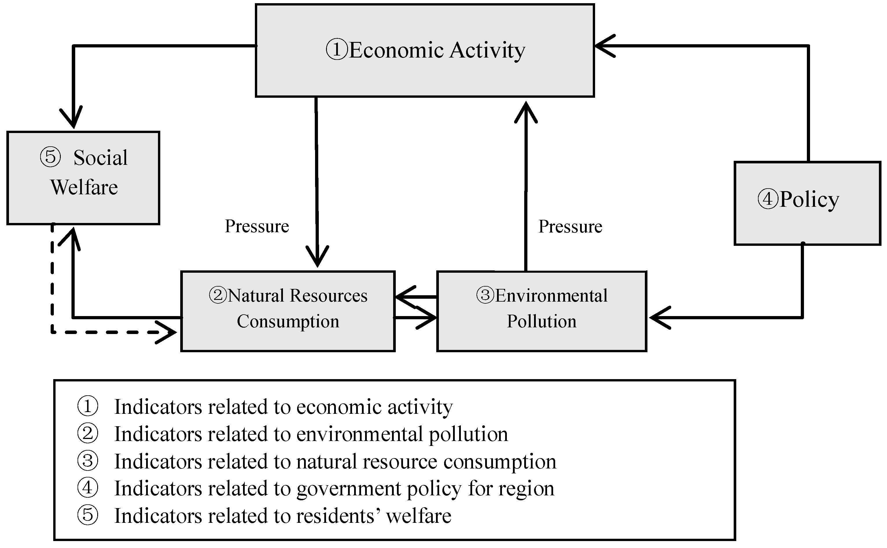
Indicator selection entails deciding on a framework to guide measurement of green growth and then ensuring that the set of indicators chosen covers all aspects of this framework. The OECD has outlined a framework that includes three categories: economic activity, natural resources and environment, and social welfare [27]. This study divided the natural resources and environment category of the OECD framework into two independent measurement categories: natural resources consumption and environmental pollution. Due to the dominant characteristics of China’s politics, policy (like investments policy, innovation policy, and so on) is an important driving force of economic development in China [28] and has been added into the framework as an independent dimension. Additionally, according to the OECD green growth strategy and policy characteristics of China, in the course of this study the framework of green growth with five interrelated measurement dimensions was built: (1) Economic activity indicators related to economic activity arising from production and consumption express the health of the economic growth of the measured region. (2) Natural resources consumption indicators related to resource consumption resulting from economic activity. (3) Environmental pollution indicators related to the pollution caused by economic activity. (4) Policy indicators related to government regulation. (5) Social welfare indicators related to residents’ welfare (Figure 1).

2.2. The Green Growth Indicator System

Based on the established framework, the indicators of green growth are selected for scientific evaluation. To provide comprehensive support for policy decisions related to the green growth problem and to underline this study’s contributions, the indicators in this study are divided into two types: general indicators, frequently used by the OECD and other researches focused on green growth; and proprietary indicators, which represent the unique characteristics of the studied regions. With respect to the general indicators, natural resources and environment are invariable core elements in the study of green issues [6]. The OECD has suggested energy use per unit of GDP (labeled as P5), proportion of land covered by forest (labeled as P6), and withdrawal of surface and groundwater of total available water as crucial indicators of energy consumption and natural capital [2,29]. Because of the difference of statistical caliber, water consumption per capita (labeled as P7) is used as an indicator of water consumption in China [10,14]. In terms of environmental pollution, waste gas, waste water, and solid waste are the three main threats to the environment. Sulfur dioxide emissions (labeled as P8) and smoke and dust emissions (labeled as P9) are widely recognized indicators for measuring exhaust gases; similarly, wastewater emissions (labeled as P10) is a credible indicator for measuring waste water, and a general indicator for measuring the comprehensive utilization of solid wastes is the comprehensive utilization rate of industrial solid waste (labeled as P11) [12]. Research and development (R&D) expenditure accounts for the proportion of GDP (labeled as P12), government environmental protection expenditure as a percentage of GDP (labeled as P13), and sewage treatment rate (labeled as P14) are the essential indicators in studying green growth-related policies. For example, Samad selected intellectual property rights, R&D expenditure accounts for the proportion of GDP, and environmental taxes and fees as important indicators of green innovation, reflecting the government’s support for green patent technology and green growth [30]. Ploeg thought that R&D subsidy is an effective economic incentive with which to achieve cleaner production [31].

To measure green growth in China, the indicator of China’s economic activity and social welfare is the key to the indicator selection process. The healthy growth of the economy is the prerequisite for the whole development [15]. The economy activities form the basis for successful green growth. GDP is the most direct expression of a country’s economic strength. Due to the region difference in China, the per capita GDP (labeled as P1) is a symbol of regional economic strength. For example, Lorek selected population numbers, per capita GDP, and energy consumption per unit GDP to build environmental pressure formula and studied the development direction of sustainable consumption from the perspective of green growth and green economy [32]. Natural population growth rate (labeled as P2) and urbanization rate (labeled as P3) are important symbols of vitality in a region [2,33]. Urbanization is the way to modernize; promoting urbanization rate is an important way to solve the problems of agriculture, rural areas, and farmers, and is a powerful support to promote the coordinated development of China [3,13]. Several studies have proposed that effective economy growth is mainly driven by the output value created by industry. The added industrial value is the final result of industrial production activities, which can reflect the industrial economic strength of the region in a certain stage by the industrial value added as a share of GDP (labeled as P4) [4]. China is still a country based on industrial production. Measuring China’s economic development is inseparable from the calculation of industrial output value [2]. Social welfare is reflected in the basic necessities of life and the living security of the residents. In China, education funds mainly refer to the cost of the state for the development of education at all levels [17]. Education expenditure accounts as a proportion of GDP (labeled as P15) can reflect the importance of the country’s attention to education, which is an important manifestation of the level of the residents’ education [33]. Drinking water qualification rate (labeled as P16) and innocuous treatment rate of domestic waste (labeled as P17) are the guarantee for basic living of residents [15,22]. “Five social insurances and one housing fund” is China’s social security system; it contains endowment insurance, medical insurance, unemployment insurance, employment injury insurance, maternity insurance, and housing provident fund [17]. Medical insurance is the core residents’ concern, and the health care spending per capita (labeled as P18) is an important indicator with which to measure residents’ security.

Based on the indicators adopted by experts and scholars in green growth evaluation, this paper constructs an evaluation indicator system with 18 indicators (

Table 1. China’s green growth indicator system (Source: Modified by the author).

Factor	Practice	Indicator	References
Economic Activity	P1	Per capita GDP	[15,26]
	P2	Natural population growth rate	[15,32]
	P3	Urbanization rate	[3,13,34]
	P4	Industrial value added as a share of GDP	[2,4]
Natural Resources Consumption	P5	Energy use per unit of GDP	[6,26]
	P6	Proportion of land covered by forest	[11,26]
	P7	Water consumption per capita	[6,10,14,26]
Environmental Pollution	P8	Sulfur dioxide emissions	[12,26]
	P9	Smoke and dust emissions	[12,26]
	P10	Wastewater emissions	[6,12]
	P11	Comprehensive utilization rate of industrial solid waste	[2,3]
Policy	P12	R&D expenditure accounts as a proportion of GDP	[6,26]
	P13	Government environmental protection expenditure as a percentage of GDP	[6,26]
	P14	Sewage treatment rate	[15,22]
Social Welfare	P15	Education expenditure accounts as a proportion of GDP	[17,33]
	P16	Drinking water qualification rate	[3,15]
	P17	Innocuous treatment of domestic waste rate	[15,22]
	P18	Health care spending per capita	[17]

).

3. Methodology

In order to track the green growth index in China, the entropy method is widely used to calculate the indicator’s weight details. The regional Gini coefficient and the coefficient of variation enable one to determine differences in geographical space. The Exploratory Spatial Data Analysis (ESDA) can calculate the degree of spatial agglomeration.

3.1. Setting the Indicator’s Weight and Green Growth Index Calculation

The calculation of Green Growth Index (GGI) is the premise of the following analysis. Based on the green growth indicator system obtained in Section 2, the green growth index of each region in this paper is calculated. The indicator’s weight has important influence on the evaluation of regional green growth. This paper employs entropy method to calculate the objective weight of the evaluation indicator (w_j) [34]. The calculation formula of entropy method is as follows:

$$w_j^{}=(1-e_i)/(m-{\displaystyle \sum _{i=1}^m{e}_i),(i=1,2,\dots \dots ,m})$$

(1)

$$e_i=-\frac{1}{\ln n}{\displaystyle \sum _{j=1}^n{p}_{ij}\ln (p_{ij})}$$

(2)

in which $p_{ij}$ is the value after the standardization of the j indicator in the year i.

Finally, the Green Growth Index (GGI) of each region is expressed as

$$GGI={\displaystyle \sum _{i=1}^n{p}_j{w}_j}$$

(3)

in which GGI represents the index of regional green growth, p_j represents the standardized value of each year i, w_j is the weight of each indicator, and n is the number of the indicator [34].

3.2. The Regional Gini Coefficient

The Gini coefficient was used in the study of social income inequality. The Regional Gini Coefficient (RGC), as an application of the Gini coefficient in economics, is used to analyze the agglomeration degree of various economic and social phenomena in a geographical space [35]. The greater the regional Gini coefficient is, the higher the degree of spatial agglomeration. The calculation formula of the regional Gini coefficient is as follows:

$$RGC=\frac{1}{2n^2\overline{GGI}}{\displaystyle \sum _{i=1}^n{\displaystyle \sum _{j=1}^n\left|GG{I}_i-GG{I}_j\right|}}$$

(4)

in which n is the number of research region and GGI is the index of the regional green growth.

3.3. The Coefficient of Variation

The Coefficient of Variation (CV) is a relative quantity that represents the standard deviation relative to the average number. It reflects the evaluation results for the average of the relative degree of dispersion [17]. It is an index for analyzing regional differences. The greater the CV is, the bigger the difference is. The calculation formula is

$$CV=\frac{\sqrt{{\displaystyle \sum _i^n(GG{I}_i-{\overline{GGI})}^2}/n}}{\overline{GGI}}$$

(5)

in which n is the number of the research region and GGI is the index of the regional green growth.

3.4. The Exploratory Spatial Data Analysis

The Exploratory Spatial Data Analysis (ESDA) represents as a series of techniques that are used to statistically analyze spatial data and acquire necessary knowledge as to spatial structure and correlation [36]. The core of ESDA is the spatial autocorrelation measure. Spatial autocorrelation is an important index with which to test whether the attribute values of a certain element are significantly associated with the attribute values on the adjacent spatial points. As a kind of recognition function of spatial data analysis method, the ESDA is divided into global spatial autocorrelation and local spatial autocorrelation [20].

3.4.1. The Global Spatial Autocorrelation

The global spatial autocorrelation is an overall statistical index, which is mainly used to measure the spatial association mode of the whole region, reflecting the similarity of the observation values of the spatial adjacent area, in order to determine whether there is a cluster phenomenon in the space. The global Moran’s I is used to analyze the differences in the degree of spatial statistics to estimate the overall regional association and space by using the following calculation method [36]:

$$\mathrm{Moran}’\mathrm{s}I=\frac{{\displaystyle \sum _{i=1}^n{\displaystyle \sum _{j=1}^n{W}_{ij}(GG{I}_i-\overline{GGI})(GG{I}_j-\overline{GGI})}}}{S^2{\displaystyle \sum _{i=1}^n{\displaystyle \sum _{i=1}^n{W}_{ij}}}}$$

(6)

$S^2=\frac{1}{n}{\displaystyle \sum _{i=1}^n(GG{I}_i-\overline{GGI})}$, in which n is the total number of regions in the study area and W_ij is the spatial weight. The significance of the Moran’s I index can be tested by standardized Z statistics, which are as follows:

$$\mathrm{Z}=\frac{I-E(I)}{SD(I)}$$

in which I is the Moran’s I index, E(I) is the expected mean, and the SD(I) is the expected variance. If the Z value is greater than the critical value of normal distribution function at 0.01 levels, there is a spatial correlation between regions, and if not, there is no spatial correlation. The value of the global Moran’s I index is generally between −1 and 1. When the global Moran’s I > 0, there is a positive correlation between the regions; the higher the global Moran’s I is, the stronger the positive autocorrelation. Otherwise, when the global Moran’s I < 0, there is a negative correlation between the regions and a scattered pattern in space [16]. When the global Moran’s I is close to 1, the areas with similar attributes are clustered together. When the global Moran’s I is close to −1, the areas with distinct properties are clustered together.

3.4.2. The Local Spatial Autocorrelation

Local spatial autocorrelation analysis indicators can be more comprehensive to reflect the change trend of local spatial differences, the Moran plot, and Local Moran I statistics analysis between each region and the surrounding areas of the space pattern and difference degree [37]. The local Moran I statistics is the decomposition of the global Moran’s I, which is used to measure the spatial difference of the green growth between the region i and its surrounding region. The specific form is

$$I_i=z_i{\displaystyle \sum _{j=1}^n{w}_{ij}{z}_j}$$

(7)

in which z_i and z_j are standardized spatial parameter observations. The Moran scatter diagram can directly show the spatial correlation effect of different regions. The four quadrants are used to show four spatial statuses.

(1) “High-High (H-H)” level indicates that areas with a high green growth level are surrounded by other high green growth level areas with little spatial difference among regions and strong positive spatial correlation. The regions in H-H level have strong green growth ability and are easy to generate green growth spillover effect to drive the development of surrounding areas; (2) “Low-High (L-H)” level indicates that a high green growth level area is surrounded by a low green growth level area with large spatial difference and strong negative spatial correlation; (3) “Low-Low (L-L)” level shows both the region and surrounding region are low green growth level regions with a small spatial difference. The regions in L-L level have weak green growth ability and focus on the national policy (4). “High-Low (H-L)” level indicates that the area with high green growth level is adjacent to other regions with low green growth level; there is a large spatial difference and a strong negative correlation of space. This region is highly susceptible to the positive development of the surrounding area [34].

4. Data Analysis and Results

4.1. Data Resources

This paper presents data for 30 out of 34 provinces of China, Hong Kong, Macao, Taiwan, and Tibet that are not selected as the study areas. The data for Hong Kong, Macao, and Taiwan cannot be used for determining the difference of the statistical standard of the “One Country, Two Systems” policy, whereas the data for Tibet are not available. The data for the remaining 30 provinces are derived from China Regional Statistical Yearbook (2006–2015), China Environmental Statistics Yearbook (2006–2015), and China Energy Statistics Yearbook (2006–2015) [10].

4.2. The General Characteristics of Green Growth

The changes of green growth index as to time and space are explained in

Table 2. Regional Green Growth Index from 2005 to 2014 (source: modified by the author).

GGI	2005	2006	2007	2008	2009	2010	2011	2012	2013	2014
BeiJing (BJ)	0.657	0.724	0.716	0.729	0.802	0.789	0.811	0.852	0.882	0.901
TianJin (TJ)	0.548	0.577	0.562	0.576	0.605	0.622	0.644	0.669	0.687	0.706
Hebei (HE)	0.298	0.334	0.355	0.406	0.445	0.471	0.461	0.484	0.494	0.531
ShanXi (SX)	0.257	0.297	0.346	0.405	0.466	0.499	0.490	0.562	0.574	0.604
NeiMenggu (NM)	0.230	0.276	0.330	0.364	0.405	0.448	0.479	0.516	0.531	0.577
LiaoNing (LN)	0.359	0.381	0.396	0.435	0.467	0.494	0.507	0.570	0.544	0.532
JiLin (JL)	0.323	0.359	0.393	0.399	0.435	0.470	0.464	0.484	0.504	0.521
HeiLongjiang (HL)	0.304	0.330	0.351	0.387	0.429	0.461	0.462	0.504	0.528	0.528
ShangHai (SH)	0.494	0.580	0.608	0.613	0.662	0.646	0.646	0.689	0.709	0.716
JiangSu (JS)	0.467	0.482	0.493	0.517	0.538	0.550	0.541	0.568	0.597	0.605
ZheJiang (ZJ)	0.444	0.478	0.493	0.566	0.558	0.581	0.568	0.616	0.634	0.663
AnHui (AH)	0.306	0.371	0.414	0.440	0.465	0.487	0.511	0.545	0.583	0.588
FuJian (FJ)	0.408	0.425	0.441	0.486	0.534	0.555	0.564	0.609	0.627	0.627
JiangXi (JX)	0.257	0.314	0.361	0.394	0.445	0.488	0.517	0.550	0.539	0.565
ShanDong (SD)	0.386	0.407	0.438	0.474	0.517	0.531	0.523	0.571	0.596	0.610
HenAn (HA)	0.286	0.304	0.333	0.373	0.409	0.433	0.428	0.473	0.499	0.543
HeBei (HB)	0.372	0.392	0.410	0.442	0.470	0.498	0.514	0.549	0.563	0.584
Hunan (HU)	0.329	0.357	0.384	0.415	0.455	0.474	0.479	0.529	0.530	0.548
GuangDong (GD)	0.371	0.426	0.442	0.482	0.508	0.570	0.529	0.537	0.578	0.595
GuangXi (GX)	0.283	0.321	0.346	0.363	0.422	0.444	0.470	0.521	0.526	0.466
HaiNan (HN)	0.385	0.462	0.494	0.525	0.530	0.565	0.574	0.618	0.603	0.579
ChongQing (CQ)	0.293	0.346	0.433	0.492	0.519	0.559	0.581	0.596	0.610	0.608
SiChuan (SC)	0.283	0.335	0.356	0.400	0.422	0.439	0.458	0.474	0.508	0.587
GuiZhou (GZ)	0.190	0.243	0.281	0.311	0.336	0.403	0.461	0.498	0.514	0.570
YunNan (YN)	0.251	0.283	0.337	0.391	0.435	0.476	0.488	0.520	0.538	0.530
ShaNxi (SN)	0.265	0.372	0.395	0.423	0.484	0.517	0.527	0.564	0.570	0.606
GanSu (GS)	0.223	0.270	0.287	0.313	0.342	0.399	0.423	0.494	0.522	0.543
QingHai (QH)	0.231	0.297	0.331	0.364	0.381	0.416	0.481	0.510	0.519	0.538
NingXia (NX)	0.267	0.334	0.429	0.450	0.452	0.498	0.514	0.537	0.563	0.573
XinJiang (XJ)	0.298	0.287	0.297	0.333	0.396	0.414	0.442	0.463	0.469	0.503
Average	0.335	0.379	0.408	0.442	0.478	0.507	0.519	0.556	0.571	0.588

and Figure 2, respectively. The gaps between regions, calculated with the help of the RGC and CV, are shown in Figure 3.

4.2.1. The Temporal Evolution Characteristics of the Regional Green Growth

The green growth evaluation results of 30 provinces for the years 2005 to 2014 are shown in Table 2. Regions in Table 2 are abbreviated, for example, Beijing is labeled as BJ, whereas the specific region location is shown in Figure 2. The green growth capacity of the provinces of China has been constantly improving since 2005 with increases of the GGI from 0.335 in 2005 to 0.588 in 2014; the growth rate has reached 42.9%. This shows that China’s regional green growth capacity is increasing, and the regions are paying great attention to the transformation of the regional economic growth mode to promote green growth. BJ has the most obvious growth advantage compared to other regions. The main reason for this is that BJ, as the political and administrative center of China, is the gathering place of the new developed industry. The dominant industry consists of enterprises with less resource consumption and less environmental pollution, which greatly conforms to the tenet of green growth and leads to the rapid development of this region compared to other provinces.

4.2.2. The General Spatial Evolution Characteristics of Regional Green Growth

The general spatial evolution characteristic of the regional green growth presents a horizontal expansion and a vertical extension; the dynamic change is manifested in the movement from the east to the west, from the central part to the northern and southern regions. Figure 2 demonstrates the green growth evaluation results (Table 2) in the spatial presentation; the darker the color is, the higher the green growth level. According to the color change trend in Figure 2, it can be determined that the green growth level in the years 2005 to 2014 gradually spread from the eastern to the western region (the color gradually deepens with time in the central and western regions). Figure 2 also shows the trend of gradual spreading from the central region to the northwest and southwest (the color is deeper in the northwest and southwest regions of Figure 2). In particular, the eastern coastal areas’ (BJ, TJ, SD, JS, ZJ, FJ, GD, and HN) steady growth has been dominated by China’s green growth heights (these areas are marked with the deepest color). SN, NX, and CQ are the core points of the central region that drive the development of SX, NM, SC, and HB, forming a longitudinal extension of the central active zone and thus promoting the development of QH, GS, and other western regions (color from pale to deep). The northeast region is in a state of “collapse”, and its green growth level is gradually decreasing, which is represented by LN and JL. From 2005 to 2014, the green growth level had reduced from an intermediate level to the lowest level (color from deep to pale).

4.2.3. The Differences of Regional Green Growths

According to the coefficient of variation line shown in Figure 3, we can see that the coefficient of variation in every region decreased from 0.304 in 2005 to 0.135 in 2014; thus, the decline rate was 124%. The coefficient of variation is shrinking rapidly each year, which shows that the regional disparity of China’s green growth gradually reduced. Based on the regional Gini coefficient trend line, we can see that the regional Gini coefficient from 2005 to 2014 is less than 1 and gradually decreases. It shows that between the years 2005 and 2014, China’s green growth does not appear to be concentrated in a few provinces, but common development of various regions takes place, showing a trend of continuous progress. From

Table 3. Moran’s I test of the regional green growth in China (Source: Modified by the author).

Year	2005	2006	2007	2008	2009	2010	2011	2012	2013	2014
Moran’s I	0.491	0.461	0.457	0.444	0.437	0.413	0.311	0.288	0.295	0.291
Z	6.58	6.83	6.33	5.63	5.3	5.18	4.03	3.59	3.76	3.71

we can see that for the research period, the value of Moran’s I remains positive, and the mean value of Z is 5.094, which is more than 1.96 (the critical value of normal distribution function at 0.01 level). This shows that the green growth of China’s provinces from 2005 to 2014 is not a random distribution, and that there is a spatial agglomeration. The regions with high green growth level are often adjacent to the regions with a similar green growth level, showing thus “similarity” characteristics and positive spatial autocorrelation. The larger positive spatial autocorrelation also shows that the spatial difference of green growth in different regions of China is decreasing.

4.3. The Specific Spatial Transition Characteristics of Regional Green Growth

In

Table 4. Specific distribution of Moran scatter plot in China from 2005 to 2014 (source: modified by the author).

Year	H-H	L-H	L-L	H-L	Cross Region
2005	TJ, BJ, SH, JS, ZJ, FJ	JX, HE, AH	HN, CQ, GX, HL, GZ, NM, GS, QH, JX, YN, SN, NX, SC, XJ	LN, JL, HU, HB	SD (H-H, H-L) GD (H-H, H-L) HN (H-H, H-L)
2006	TJ, BJ, SH, JS, ZJ, FJ	JX, HE	LN, HN, CQ, GX, HL, GZ, NM, GS, QH, JX, YN, SN, NX, SC, XJ	SD, HB, GD	HN (H-H, H-L) AH (H-H, L-H) HU (L-L, H-L) JL (L-L, H-L)
2007	TJ, BJ, SH, JS, ZJ, FJ, AH	JX, HE	HU, LN, HN, CQ, GX, HL, GZ, NM, GS, QH, JX, YN, SN, NX, SC, XJ	SD, HB, GD, CQ	HN (H-H, H-L) JL (L-L, H-L)
2008	TJ, BJ, SH, JS, ZJ, FJ	JX, HE, AH	LN, JL, HN, CQ, GX, HL, GZ, NM, GS, QH, JX, YN, SN, NX, SC, XJ	SD, HB, GD, CQ	HU (L-L, H-L) HN (H-H, H-L)
2009	TJ, BJ, SH, JS, ZJ, FJ	JX, HE, AH	HB, HU, LN, JL, HN, CQ, GX, HL, GZ, NM, GS, QH, JX, YN, SN, NX, SC, XJ	SD, CQ	HN (H-H, H-L) GD (H-H, H-L)
2010	TJ, BJ, SH, JS, ZJ, FJ	JX, HE, AH	HB, HU, LN, JL, HN, CQ, GX, HL, GZ, NM, GS, QH, JX, YN, SN, NX, SC, XJ	SD, CQ	HN (H-H, H-L) GD (H-H, H-L)
2011	TJ, BJ, SH, JS, ZJ, FJ	JX, HE	HB, LN, JL, HN, CQ, GX, HL, GZ, NM, GS, QH, JX, YN, NX, SC, XJ	CQ	HN (H-H, H-L) GD (H-H, H-L) SN (L-L, H-L) SD (L-L, H-L) HU (L-L, L-H) AH (L-L, L-H)
2012	TJ, BJ, SH, JS, ZJ, FJ	JX, HE	HB, HU, LN, JL, HN, CQ, GX, HL, GZ, NM, GS, QH, JX, YN, NX, SC, XJ	SD, SN, CQ	AH (L-L, L-H) GD (H-H, L-H) HN (H-H, H-L)
2013	TJ, BJ, SH, JS, ZJ, FJ	JX, HE	LN, JL, HN, CQ, GX, HL, GZ, NM, GS, QH, JX, YN, NX, SC, XJ	SD, SN, CQ	GD (H-H, L-H) HN (H-H, H-L) AH (L-L, L-H) HU (L-L, L-H) HB (L-L, H-L)
2014	TJ, BJ, SH, JS, ZJ, FJ	JX, HE, AH	HU, LN, JL, CQ, GX, HL, GZ, NM, GS, QH, YN, NX, SC, XJ	SD, SN, CQ, GD, JX	HN (L-H, L-L) HB (H-H, H-L, L-H) HN (H-H, H-L)

we can see the spatial transition of green growth index in different provinces and find that most of the provinces showed significant positive spatial autocorrelation. Most provinces are located in H-H and L-L level areas, but the proportion of L-L provinces (14 provinces) is significantly higher than the H-H provinces (6 provinces). Specifically, the following two changes were found in the green growth transition of different regions.

4.3.1. The Spatial Pattern of Green Growth is Stable, and There Is No Obvious Transition Phenomenon in 22 Provinces

From the years 2005 to 2014, 22 provinces (73% of the total number) showed continuous spatial stability. Among them, 6 provinces (BJ, TJ, SH, JS, ZJ, and FJ) are always located in H-H level areas. The regions have a high level of green growth and are slightly different from the surrounding area. It has always been the case in the central areas, showing a strong agglomeration phenomenon. Thirteen provinces, namely, HA, GX, HL, LN, GZ, NM, GS, QH, SX, YN, NX, SC, and XJ, are located in the third quadrant. Such area has a low green growth level and small diffusion characteristics, demonstrating a weak agglomeration phenomenon. JX and HE are located in the second quadrant; their green growth ability is weak, whereas the difference between them is large, and the weak polarization effect is prominent. SD is located in the fourth quadrant with strong green growth capability, which is, however, weak in its surrounding areas. The above results show that the spatial relationship pattern of China’s provincial green growth has not changed significantly from 2005 to 2014.

4.3.2. The Eastern and Central Parts of the Country Will Continue to Be Active, and the Northeast Inertia Will Collapse

Compared with the continuous stability of the 22 provinces, 8 provinces (GD, CQ, SX, HU, SN, HB, AH, and JL) exhibited spatial activity. The area of GD, for instance, had been changing its status from H-H to H-L, had a weak impact on the surrounding areas, and did not a strong green spillover effect. It is determined that GD, GX, HU, and JX are located in weak green growth. CQ and SN as the gateways to the central and western regions all changed their status from L-L to H-L, showing a strong green spillover effect and driving the development of neighboring regions, namely, SC, NX, and SX. The spatial spillover effect of these two regions is obvious, and the transformation from weak aggregation to strong heterogeneity took place, which led to the improvement of green growth throughout the central region. In 2014, the central and north-central regions reached a strong green growth level (the deepest in color). HB changed its status from H-L to L-L in 2008. AH changed its status from H-H to L-H in 2008 and from L-H to L-L since 2011, and then hovered between L-L and L-H. The two regions are located in the middle zone between the strong agglomeration area (JS, SH, ZJ, etc.) and the weak agglomeration area (HA, HE, and HB). Since 2005, JL has changed from a strong zone to a weak agglomeration area; its own advantage is weakening, and the surrounding HL, LN, and other provinces have been in L-L level, showing the development trend of inert collapse.

Finally, summarize the future development trend: Most of the eastern coastal provinces are in the H-H stage, with strong momentum of development. The provinces CQ and SN are the central points that drive the active development of the surrounding provinces and have already drawn the northern provinces to enter the green growth strong area. The western regions are driven by the neighboring provinces of the central region and are at an embryonic stage of green growth. The stagnation in the northeastern region is obvious and has shown the development trend of inert collapse.

5. Conclusions

This paper, based on the concept and framework of OECD on green growth, introduced the measure framework and indicator system to evaluate the green growth level in 30 provinces of China for the years 2005 to 2014, and determined the status and spatial evolution characteristics of green growth in China.

From the time perspective, China’s green growth capacity has been continuously improving from 2005 to 2014. In view of the spatial pattern change, the gap between regional green growths is narrowing. The spatial pattern is extending from the developed eastern region to the backward western region and spreading from central region to the northwestern and southwestern regions. There is a significant green growth spillover, which affects the adjacent regions. Each region has made efforts to enhance its green growth and transformed the regional economic growth mode into green growth.

With respect to the spatial dynamic relationship pattern, there is no obvious transition phenomenon in 22 provinces, which indicates that the overall spatial relationship pattern of China’s provincial green growth is stable. However, there are still 8 provinces showing spatial activity. CQ and SX, as positively active areas in the central region, have shown strong green growth spillover effects, driving the central and western regions to achieve green growth. As a representative of the negatively active areas in northeast China, JL changes its level from H-L to L-L, and its ability with regard to green growth gradually becomes weaker. Since the other two regions in northeastern China were at L-L level, this region may collapse in the future.

Based on the empirical results, the following implications are drawn for different types of regions. (1) For the active eastern coastal region and the central region, preferential policy subsides will be more conductive to their outward investment. The eastern region has the most high-tech industrial clusters in China. The central region is rich in resources, and strong in industry and agriculture; it is a bridge linking the east with the west. Encouraging enterprises to build factories in other regions will drive backward areas to enhance their technological innovation and promote employment. (2) It is likely that the inactive northeastern region of China will be the future focus area and a region with a preference for dividend policy. Encouraging investment and introducing technology through policy advantages to promote industrial transformation in the region is the main direction of its future development.

However, the research upon which this paper is based is the indicator system and has some limitations. Firstly, only the key indicators are selected while measuring green growth. For example, for the natural resources consumption category, the indicators of water and energy consumption were the key choices in order to highlight the characteristics of resource restrictions, whereas the utilization of renewable energy was of less importance. In terms of the economic activity category, in order to emphasize the importance of economic growth, fewer indicators have focused on the output related indicators of green products, such as patents in environment-related technology. Secondly, this research relied on a small-scale green growth expert committee; further research should consider the opinions of experts in other fields. In the future, a more comprehensive evaluation index system should be chosen as far as possible for green growth measurement, and the qualitative and quantitative screening of the indicators will be carried out in order to obtain more scientific results.

References

- Gazheli, A.; van den Bergh, J.; Antal, M. How realistic is green growth? Sectoral-level carbon intensity versus productivity. J. Clean. Prod. 2016, 129, 449–467. [Google Scholar] [CrossRef]
- Kang, Y.; Xie, B.; Wang, J.; Wang, Y. Environmental assessment and investment strategy for China’s manufacturing industry: A non-radial DEA based analysis. J. Clean. Prod. 2018, 175, 501–511. [Google Scholar] [CrossRef]
- Dai, H.; Xie, X.; Xie, Y.; Liu, J.; Masui, T. Green growth: The economic impacts of large-scale renewable energy development in China. Appl. Energy 2016, 162, 435–449. [Google Scholar] [CrossRef]
- Guo, L.; Qu, Y.; Wu, C.; Wang, X. Identifying a pathway towards green growth of Chinese industrial regions based on a system dynamics approach. Resour. Conserv. Recycl. 2018, 128, 143–154. [Google Scholar] [CrossRef]
- Jouvet, P.; de Perthuis, C. Green growth: From intention to implementation. Int. Econ. 2013, 134, 29–55. [Google Scholar] [CrossRef]
- Kim, S.E.; Kim, H.; Chae, Y. A new approach to measuring green growth: Application to the OECD and Korea. Futures 2014, 63, 37–48. [Google Scholar] [CrossRef]
- Kokkaew, N.; Rudjanakanoknad, J. Green assessment of Thailand’s highway infrastructure: A Green Growth Index approach. KSCE J. Civ. Eng. 2017, 21, 2526–2537. [Google Scholar] [CrossRef]
- Ackah, I.; Kizys, R. Green growth in oil producing African countries: A panel data analysis of renewable energy demand. Renew. Sustain. Energy Rev. 2015, 50, 1157–1166. [Google Scholar] [CrossRef] [Green Version]
- Hafeznia, H.; Pourfayaz, F.; Maleki, A. An assessment of Iran’s natural gas potential for transition toward low-carbon economy. Renew. Sustain. Energy Rev. 2017, 79, 71–81. [Google Scholar] [CrossRef]
- Guo, L.L.; Qu, Y.; Tseng, M. The interaction effects of environmental regulation and technological innovation on regional green growth performance. J. Clean. Prod. 2017, 162, 894–902. [Google Scholar] [CrossRef]
- Song, M.; Wang, S. Measuring environment-biased technological progress considering energy saving and emission reduction. Process Saf. Environ. Prot. 2018, 116, 745–753. [Google Scholar] [CrossRef]
- Lyytimäki, J.; Antikainen, R.; Hokkanen, J.; Koskela, S.; Kurppa, S.; Känkänen, R.; Seppälä, J. Developing Key Indicators of Green Growth. Sustain. Dev. 2018, 26, 51–64. [Google Scholar] [CrossRef]
- Guo, L.; Qu, Y.; Wu, C.; Gui, S. Evaluating Green Growth Practices: Empirical Evidence from China. Sustain. Dev. 2018. [Google Scholar] [CrossRef]
- Zhao, T.; Yang, Z. Towards green growth and management: Relative efficiency and gaps of Chinese cities. Renew. Sustain. Energy Rev. 2017, 80, 481–494. [Google Scholar] [CrossRef]
- Sun, X.; Liu, X.; Li, F.; Tao, Y.; Song, Y. Comprehensive evaluation of different scale cities’ sustainable development for economy, society, and ecological infrastructure in China. J. Clean. Prod. 2017, 163, S329–S337. [Google Scholar] [CrossRef]
- Ma, F.; Wang, W.; Sun, Q. Ecological Pressure of Carbon Footprint in Passenger Transport: Spatial-Temporal Changes and Regional Disparities. Sustainability 2018, 10, 317. [Google Scholar] [CrossRef]
- Guo, Y.; Wang, H.; Nijkamp, P.; Xu, J. Space-time indicators in interdependent urban-environmental systems: A study on the Huai River Basin in China. Habitat Int. 2015, 45, 135–146. [Google Scholar] [CrossRef]
- Holt, A.R.; Mears, M.; Maltby, L.; Warren, P. Understanding spatial patterns in the production of multiple urban ecosystem services. Ecosyst. Serv. 2015, 16, 33–46. [Google Scholar] [CrossRef]
- Chen, B.; Yang, Q.; Zhou, S.; Li, J.S.; Chen, G.Q. Urban economy’s carbon flow through external trade: Spatial-temporal evolution for Macao. Energy Policy 2017, 110, 69–78. [Google Scholar] [CrossRef]
- Xu, T.; Zhu, C.; Shi, L.; Gao, L.; Zhang, M. Evaluating energy efficiency of public institutions in China. Resour. Conserv. Recycl. 2017, 125, 17–24. [Google Scholar] [CrossRef]
- Hu, X.; Hong, W.; Qiu, R.; Hong, T.; Chen, C.; Wu, C. Geographic variations of ecosystem service intensity in Fuzhou City, China. Sci. Total Environ. 2015, 512–513, 215–226. [Google Scholar] [CrossRef] [PubMed]
- Liu, H.; Fang, C.; Zhang, X.; Wang, Z.; Bao, C.; Li, F. The effect of natural and anthropogenic factors on haze pollution in Chinese cities: A spatial econometrics approach. J. Clean. Prod. 2017, 165, 323–333. [Google Scholar] [CrossRef]
- Schmalensee, R. From “Green Growth” to sound policies: An overview. Energy Econ. 2012, 34, S2–S6. [Google Scholar] [CrossRef] [Green Version]
- Slunge, D.; Loayza, F. Greening growth through strategic environmental assessment of sector refoms. Public Adm. Dev. 2012, 32, 245–261. [Google Scholar] [CrossRef]
- Stoknes, P.E.; Rockström, J. Redefining green growth within planetary boundaries. Energy Res. Soc. Sci. 2018, 44, 41–49. [Google Scholar] [CrossRef]
- OECD. Towards Green Growth: A Summary for Policy Makers; OECD: Paris, France, 2011. [Google Scholar]
- Saufi, N.A.A.; Daud, S.; Hassan, H. Green Growth and Corporate Sustainability Performance. Procedia Econ. Financ. 2016, 35, 374–378. [Google Scholar] [CrossRef]
- Cheng, Z.; Li, W. Independent R and D, Technology Introduction, and Green Growth in China’s Manufacturing. Sustainability 2018, 10, 311. [Google Scholar] [CrossRef]
- Bowen, A.; Hepburn, C. Green growth: An assessment. Oxf. Rev. Econ. Policy 2015, 30, 407–422. [Google Scholar] [CrossRef]
- Samad, G.; Manzoor, R. Green growth: Important determinant. Singap. Econ. Rev. 2015, 60, 1550014. [Google Scholar] [CrossRef]
- Van der Ploeg, R.; Withagen, C. Green Growth, Green Paradox and the global economic crisis. Environ. Innov. Soc. Transit. 2013, 6, 116–119. [Google Scholar] [CrossRef]
- Lorek, S.; Spangenberg, J.H. Sustainable consumption within a sustainable economy—Beyond green growth and green economies. J. Clean. Prod. 2014, 63, 33–44. [Google Scholar] [CrossRef]
- Barbier, E.B. Is green growth relevant for poor economies? Resour. Energy Econ. 2016, 45, 178–191. [Google Scholar] [CrossRef]
- Zhang, W.; Wang, M.Y. Spatial-temporal characteristics and determinants of land urbanization quality in China: Evidence from 285 prefecture-level cities. Sustain. Cities Soc. 2018, 38, 70–79. [Google Scholar] [CrossRef]
- Yue, W.; Zhang, Y.; Ye, X.; Cheng, Y.; Leipnik, M. Dynamics of Multi-Scale Intra-Provincial Regional Inequality in Zhejiang, China. Sustainability 2014, 6, 5763–5784. [Google Scholar] [CrossRef] [Green Version]
- Dou, Y.; Luo, X.; Dong, L.; Wu, C.; Liang, H.; Ren, J. An empirical study on transit-oriented low-carbon urban land use planning: Exploratory Spatial Data Analysis (ESDA) on Shanghai, China. Habitat Int. 2016, 53, 379–389. [Google Scholar] [CrossRef]
- Deng, X.; Xu, Y.; Han, L.; Yang, M.; Yang, L.; Song, S.; Li, G.; Wang, Y. Spatial-temporal evolution of the distribution pattern of river systems in the plain river network region of the Taihu Basin, China. Quat. Int. 2016, 392, 178–186. [Google Scholar] [CrossRef]
Figure 1.
Measurement framework of green growth (source: modified by the author based on the OECD framework [4]).
Figure 2.
Spatial Distribution Map of the Regional Green Growth Evaluation of China (source: modified by the author).
Figure 3.
Regional Gini Coefficient and the Coefficient of Variation in China for the years 2005 to 2014 (source: modified by the author).