Article

Carbon Emission Intensity, Economic Development and Energy Factors in 19 G20 Countries: Empirical Analysis Based on a Heterogeneous Panel from 1990 to 2015

1
School of Economics and Management, North China Electric Power University, Beijing 102206, China
2
Beijing Key Laboratory of New Energy and Low-Carbon Development (North China Electric Power University), Changping, Beijing 102206, China
*
Author to whom correspondence should be addressed.
Sustainability 2018, 10(7), 2330; https://doi.org/10.3390/su10072330
Submission received: 5 June 2018 / Revised: 29 June 2018 / Accepted: 30 June 2018 / Published: 5 July 2018

Abstract

:
The increasing global climate problem caused by excessive carbon emissions results in global carbon emission reduction governance becoming a top priority and requires close international coordination. Group of Twenty (G20) is gradually becoming the leading agency of global carbon emission reduction governance, but the unbalanced development among G20 countries has hindered the full play of G20’s role. Thus, this paper aims to examine the interrelationships among economic development mode, economic development level, and energy factors including energy use efficiency and structure in 19 G20 countries over the period 1990–2015. Considering the panel heterogeneity and the endogeneity of variables, a series of heterogeneous panel analysis techniques are employed in this paper. The empirical findings suggest that for the panel, the improvement of energy use efficiency and the optimization of energy use structure can help to achieve a low-carbon development mode, implying that some international agreements such as the Copenhagen Accord and Paris Agreement on Climate Change are necessary, binding, and effective. However, for individuals, energy factors and development level influence development mode differently across countries, revealing that each country should formulate specific policies that are consistent with its own actual situation. Finally, this paper discusses the role that G20 can play in the global carbon emissions reduction governance, which provides a reference for global low-carbon and sustainable development.

1. Introduction

Energy consumption is the inevitable supplementary of the development of an economy, but it also produces a lot of carbon dioxide (CO2). Therefore, the interrelationships among energy consumption, economic growth, and environmental issues like CO2 emissions, have become a hot spot for researchers trying to solve the environmental problems without hindering economic development. Many scholars tried their best to explore the relationships among energy consumption, economic growth, and CO2 emissions, and obtained rich outcomes [1,2,3,4,5]. The four hypotheses have been suggested by many researchers [3,4,5,6]. However, the academic community has not reached a unanimous conclusion about the direction of causality between economic development and energy use, although numerous studies revealed that energy use can promote economic development and CO2 emissions [5,6,7,8]. Besides, it is hard work to employ appropriate methods to describe the quantitative relationships among the three variables. Normally, most investigators tend to use econometric analysis techniques to complete this work, because of the objectivity of the results and the rigor of the theory [9,10].
Among the studies focusing on describing the quantitative relations among CO2 emissions, economic growth, and energy consumption, gross national product (GNP) was first adopted to measure the economic growth [1,2]. After that, gross domestic product (GDP) was widely used as the representative variable of economic growth [3]. Besides, some studies used per capita GDP (PCGDP) to express economic growth [4,7]. For energy consumption, the early researchers usually applied the total energy consumption (TEC) or TEC per capita in their studies [6,9], whose results were a bit indistinct and lack more in-depth descriptions. Hence, some scholars began to use more specific variables to represent energy consumption, like total fossil energy consumption (FEC) [10,11], non-renewable energy consumption (NEC) [12], and renewable energy consumption (REC) [13]. Furthermore, some researchers took the selected type of energy consumption as the analyzed variable, such as coal consumption [14], natural gas consumption [15], nuclear [16], and electricity [17], making the results more concrete and more realistic to reflect the specific relations among CO2 emissions, energy use, and economic growth. For CO2 emissions, most investigators employed the total CO2 emissions from energy [18], while some other scholars considered the total anthropogenic CO2 emissions [19] or the CO2 emissions per capita [20]. In fact, no matter which variable is used, a reasonable explanation of the results is essential.
There are two sets of common econometric methods used to describe the relationship among CO2 emissions, energy use, and economic growth, namely time-series analysis methods and panel analysis methods. Every set of methods has been widely used by many researchers for different research objects. For time-series analysis methods, which aim to describe the quantitative relationship among the variables of one object, like China [21], America [22], and Japan [23], a unit root test is necessary before investigating the nexus among the variables, in order to prevent spurious regression. After that, the two kinds of cointegration tests, namely the E–G cointegration test used for two variables and the Johansen test used for over two variables, are widely adopted to examine the long-term equilibrium among the variables. Finally, the causal relationships among variables are tested via Granger causality test technique [24,25,26]. Furthermore, some advanced approaches, like Zivot and Andrews (ZA) unit root test, autoregressive distributed lag (ARDL) approach, Gregory and Hansen cointegration test, and Toda and Yamamoto (T–Y) causality test, are also widely used in some specific situations [9,27].
For panel analysis methods, which aim to examine the quantitative relationship among the variables in multiple objects, like EU countries [28], BRICS countries [11], APEC countries [18], Central American countries [5], and so on [6,29], the cross-sectional dependence test [30,31] should firstly be completed, and then the two types of panel unit root test methods, namely the first and the second generation panel unit root tests, will be performed according to the results of the cross-sectional dependence test, in order to explore whether the panel data are stationary [31,32,33,34,35]. Next, the presence of a cointegration relationship among variables is usually examined by Pedroni panel cointegration test [36,37]. Once the presence of cointegration relationship is proven, several estimation methods, like ordinary least square (OLS), dynamic OLS (DOLS), and fully modified OLS (FMOLS) models, are widely applied to obtain the exact nexus among variables. Normally speaking, the likelihood ratio (LR) test and the Hausman test can be performed to define the form of the panel model before using the OLS approach to estimate the panel model [38]. However, because of the endogenous issues and serial correlation problems, the OLS approach is sometimes inaccurate [12]. Therefore, the FMOLS and DOLS methods are employed to obtain an accurate estimation result in some studies [12,39]. Besides, several panel Granger causality test approaches, like panel stacked Granger causality test, panel vector error correction model (VECM) causality test, and Dumitrescu–Hurlin panel causality test, are applied by many scholars [39,40], according to the characteristics of examined panel data. In order to reflect the relevant research more intuitively, the main research results are listed in Table 1, in which the methods, sample, and main findings are reported.
Recently, increasingly more scholars have believed that there are nonlinear relationships among energy, economy, and the environment, and the Environmental Kuznets Curve (EKC) model has been widely used by scholars to explore these relationships. For instance, Kaika and Zervas gave a detailed introduction to the basic concept and emergence causes of EKC, and the main research results on carbon emissions using the EKC method [41]. Liobikien and Butkus examined the impact of energy efficiency and renewable energy consumption on greenhouse gas emissions under the EKC framework, holding that increasing energy efficiency and promoting renewable energy consumption can help achieve the EKC occurrence [42]. Azam and Khan explored the EKC in four countries with different income levels and found that EKC existed in low and lower middle income countries, but no EKC was found in upper middle and high income countries [43]. Kais and Sami divided 58 countries into three regional sub-groups to explore the relationship between carbon emissions and GDP per capita in the global panel and three sub-panels, respectively, and verified that there was an inverted U-shaped curve between the two variables, that is, the EKC hypothesis was supported [44]. Bilgili et al., investigated the relationship among carbon emissions, per capita GDP, and renewable energy consumption in 17 OECD countries under the EKC framework, finding that EKC existed for the panel and was not affected by the income level of individual countries where the EKC hypothesis holds, and stating that the development of renewable energy can help to reduce carbon emissions when developing the economy [45]. Generally, the studies on the EKC framework reveal the economy–environment–energy nexus in a perspective differing from logarithmic or semi-logarithmic models, which enriches the theory and methods of studies on economy–environment–energy linkages.
In line with the above discussion, there are a series of proven methods in terms of exploring the relationships among CO2 emissions, economic development, and energy use, which are very useful references for us. However, many studies on the relationship between energy, economy, and carbon emissions are based on a linear logarithmic model, which normally adopted absolute values of CO2 emissions, economic development and energy use, whose results reflected the intuitive quantitative relationships among variables, rather than further highlighting the deep economic and social implications behind these quantitative relations, like the nexus among economic development mode, energy efficiency, energy structure, and economic development level. Besides, as the absolute values of different countries vary greatly, the panel analysis results cannot characterize the real situation of each country.
Currently, with the increasing global climate problems, the international community has placed greater emphasis on global climate governance. Among them, global carbon emission reduction governance has become a top priority. It should be noted that the realization of global carbon emission reduction targets urgently requires close international coordination and collective action, and countries in the world are not lacking the impetus to participate in global carbon emission reduction governance. However, inter-subjective game of interests, conflict of value ideas, mechanism conflicts, and the distribution of power and responsibilities are intertwined, making the global carbon emission reduction governance process falter and difficult to make breakthroughs. In particular, the institutional contradiction between the unified needs of governance and the fragmentation of governance institutions is very prominent, because the related carbon emission reduction governance organizations or institutions are scattered and dispersed, presenting a highly fragmented state of self-governance, multi-channel governance, and low-efficiency compounding, which lacks a unified governance mechanism that combines global legitimacy and enforcement efficiency.
Under the background that existing mechanisms cannot effectively meet the challenges of global carbon emission reduction governance, the Group of Twenty (G20), as the premier forum and core mechanism for global economic governance, has gradually incorporated global carbon emission reduction governance into its main agenda, has launched a series of policy measures on carbon emission reduction governance, and has gradually become the leading agency in coordinating global carbon emission reduction governance. However, there are obvious differences among G20 member states in promoting the global carbon emission reduction governance within the G20 framework, as a result of the different development modes and levels. Hence, this paper aims to adopt the panel analysis techniques to investigate the interrelationship among economic development mode, energy factors involving energy use efficiency, and structure and economic development level in 19 G20 countries, except the European Union, which can help to understand G20 countries’ dilemma in the global carbon emission reduction governance. Totally, the contributions of this paper can be concluded as below:
(1)
Most researchers use panel data when explaining the dynamic linkages among CO2 emissions, energy use, and economic development. It should be noted that the selection of panels is a main criticism for these studies. The heterogeneity of the analyzed panels of countries is non-negligible, and cross-sectional dependency may exist. Thus, this study adopts the heterogeneous panel estimation techniques considering cross-sectional dependence to complete the research.
(2)
Few literature studies the relation among economic development mode, economic development level, and energy factors in G20 countries, causing the theme of this paper to be of great theoretical and practical significance. Besides, the elasticities estimated by the panel model can reflect not only the cross-sectional nature, but also the time dimensions of the panel compared with the time-series-based studies. Moreover, the variables reflecting economic development mode, energy factors involving energy use efficiency, and structure and economic development level, like CO2 emission intensity, energy consumption intensity, fossil energy consumption share, and GDP per capita, are used in this paper. By this way, the panel estimation results can reveal the deep economic and social relationships behind the analyzed variables regardless of the sizes of the examined countries, which are helpful for policy making.
The rest of this paper is organized as follows. The data resource, descriptive statistics of variables, and model adopted in this paper are reported in Section 2. The major econometric methodologies are reported in Section 3. The empirical findings and interpretations of the results are presented in Section 4. Finally, Section 5 summarized the conclusions, puts forward several related policy remarks, and discusses the role of G20 in global carbon emission reduction governance.

2. Model, Data and Descriptive Statistics

2.1. Model and Data

As suggested by previous studies [11,18,21,22,23], energy factors and economic growth have significant effects on CO2 emissions. To explore the interrelationships among economic development mode, energy factors involving energy use efficiency, and structure and economic development level from a deeper perspective, this paper proposes a simple model where four representative variables are involved:
  C E I i t = f ( E C I i t ,   F E C S i t , P C G D P i t )
where i presents the G20 country and t is time period. CEI is the CO2 emissions intensity (kilogram per constant 2011 purchasing power parity (PPP) dollar of GDP, kg/dollar), which reflects the economic development mode; ECI is energy consumption intensity (gram of oil equivalent per constant 2011 PPP dollar of GDP, goe/dollar), which presents energy use efficiency; FECS is fossil energy consumption share (percentage of total, %), revealing energy use structure; and PCGDP is GDP per capita (constant 2011 PPP dollar, dollar), reflecting the economic development level. All of these data are collected from World Bank (http://www.worldbank.org). To avoid data fluctuations and eliminate heteroscedasticity in the panel, all variables except FECS are transformed into their natural logarithms, expressed as LCEI, LECI, and LPCGDP. Since FECS is a percentage-typed variable, its coefficient can stand for the elasticity directly.
It is worth noting that the serious economic crisis in 2008 may cause some breaks or fluctuations in the data, resulting in the apparent need for a time dummy variable. In fact, because of the variable selection and data preprocessing, the fluctuation of variables caused by the financial crisis has been effectively mitigated (Appendix A, Figure A1), and the model with a time dummy variable is proven to be not ideal (Appendix B, Table A1). Therefore, according to previous related researches [8,10,13,21], the logarithmic linear function is constructed as below:
  L C E I i t = β 1 L E C I i t + β 2 F E C S i t + β 3 L P C G D P i t + μ i t
where β 1 , β 2 , and β 3 are elasticities of CEI with respect to ECI, FECS, and PCGDP, respectively, and μ i t is the error item. In this paper, a strongly balanced panel of 19 G20 countries is applied, including South Africa (ZAF), Argentina (ARG), Brazil (BRA), Indonesia (IDN), Canada (CAN), China (CHN), Turkey (TUR), Germany (DEU), Australia (AUS), France (FRA), United Kingdom (GBR), India (IND), Italy (ITA), South Korea (KOR), Mexico (MEX), Japan (JPN), Russia (RUS), Saudi Arabia (SAU), and United States (USA), covering the period from 1990 to 2015. Although the EU is also a member of G20, it is not an independent sovereign state and is thus not included in the examined sample.

2.2. Descriptive Statistics of Variables

The descriptive statistics for the examined variables in the panel and 19 G20 countries are listed in the Appendix C (Table A2), from which it can be inferred that there is heterogeneity across countries for the variables, because the mean and median values vary in different countries. Moreover, the mean and median of most variables in each country are similar, and the p values of their Jarque-Bera (JB) [46] statistics are greater than 0.05, meaning that the hypothesis that they are normally distributed cannot be rejected at the five percent significance level. However, for the panel, the JB test rejected the null hypothesis of normal distributions for all variables, which reflects the heterogeneity across countries for the variables again.
The correlations among the studied variables in panel are presented in Table 2, indicating that CEI has positively significant correlations with ECI and FECS, but a negative correlation with PCGDP. Besides, the results also show that PCGDP has a negative correlation with ECI and a positive correlation with FECS. The correlation results for the panel data reveal that CEI and ECI are strongly related, CEI and FECS, as well as FECS and PCGDP, are moderately related, and the other variables are weakly related. Whatsoever, there is significant correlation between any two variables, indicating that it is feasible to explore the equilibrium relationship among these variables.

3. Econometric Methodologies

3.1. Cross-Sectional Dependence Test

It is worth noting that because of the regional and macroeconomic linkages that have a common impact with the world, such as the Asian financial crisis, U.S. subprime mortgage crisis, and international trade policies, cross-sectional dependence among the explored countries may exist. Therefore, it is necessary to perform a cross-sectional dependence test before performing the next works. According to Pesaran [30,31], this paper adopted the general cross-sectional dependence (CD) test in panels to examine the existence of cross-sectional dependence. Assuming that the standard panel data model is expressed as follows:
  Y i t = a i t + b i t X i t + ϵ i t
The null hypothesis supporting that there is no cross-sectional dependence is as follows: H 0 :   θ i j = θ j i = c o r ( ϵ i j , ϵ j i ) = 0 , for any i j , while the alternative hypothesis is as follows: H 1 :   θ i j = θ j i = c o r ( ϵ i j , ϵ j i ) 0 , existing i j , where θ i j is obtained by the following:
  θ i j = t = 1 T ϵ i t ϵ j t / t = 1 T ϵ i t 2 t = 1 T ϵ j t 2
According to Formula (4), the CD test statistic is as follows:
  C D = 2 T N ( N 1 ) i = 1 N 1 j = i + 1 N θ ^ i j
where θ ^ i j are the correlation coefficients calculated from the model. The CD statistic is a standard normal distribution. The null hypothesis of CD test is cross-sectional independence, while the alternative hypothesis is cross-sectional dependence.

3.2. Panel Unit Root Test

Before further empirical analysis, it is necessary to confirm the variables’ stabilities via unit root tests, aiming to prevent spurious regression. The first generation unit root tests, such as the Breitung test [32], LLC test [33], IPS test [34], PP-Fisher and ADF-Fisher test [35], are widely applied. However, for panels with a CD issue, these methods usually over-reject the null hypothesis, that is, considering an unstable sequence as a stationary sequence [30]. Thus, to accurately reflect the stationarity of sequences with cross-sectional dependence, according to Pesaran [31], a second generation unit root test approach, called a cross sectional augmented IPS (CIPS) test, is performed based on the cross-sectional augmented Dickey-Fuller (CADF) regression, which can be reported as below:
  Δ y i t = a i + b i y i , t 1 + c y ¯ t 1 + d Δ y ¯ t + ϵ i t
where y ¯ t = i = 1 n y i t / n , and Δ represents the difference operator. If there is serial correlation in the data, the extended model can be expressed as below:
  Δ y i t = a i + b i y i , t 1 + c y ¯ t 1 + j = 1 p d j Δ y ¯ t j + 1 + k = 1 p e k Δ y i , t k + ϵ i t
where p is the lagged order determined by Akaike information criterion (AIC) and Schwarz information criterion (SIC). Formula (7) presents the extended CADF regression for the i-th individual. Accordingly, the t statistic of b i can be obtained, regarded as CADFi. On this basis, the CIPS statistic is obtained by the following:
  C I P S = i = 1 n C A D F i / n
The null hypothesis of the CIPS test is that there exists unit roots, indicating that the sequence is non-stationary. By considering CD issue and heterogeneity, CIPS is regarded as a widely used second-generation panel unit root test.

3.3. Panel Cointegration Test

If the variables are of the same integrated order, it is necessary to explore the existence of a cointegration relationship among variables. Pedroni [36,37] proposed a panel cointegration test technique, according to the following formula:
  L C E I i t = α i t + β i t + γ 1 i L E C I i t + γ 2 t F E C S i t + γ i t L P C G D P i t + ε i t
where α i t and β i reflect the country-fixed and time-fixed effect, respectively; and ε i t is the residual reflecting the deviation from the long-term equilibrium. γ 1 i , γ 2 i , and γ 3 i mean the elasticities of C E I i t pertaining to E C I i t , F E C S i t , and P C G D P i t , respectively. The cointegration relationship among the analyzed variables is examined via testing the stationarity of εit, that is, for the following formula:
  ε i t = ρ i ε i , t 1 + v i t
The null hypothesis is H 0 :   ρ i = 1 , indicating that ε i t is non-stationary, that is, the studied variables are not cointegrated. Pedroni’s panel cointegration test contains seven statistics that are all of the standard normal distribution.

3.4. Panel Data Model Estimation

If the examined variables are cointegrated, determining the values of coefficients of every variable is necessary, which can reflect the long term-relationship among LCEI, LECI, FECS, and LPCGDP. For panel data, the approaches used to determine the cointegration relationship mainly include the OLS method, the FMOLS method, and the DOLS method.
The asymptotic behavior of the regression coefficients in the panel cointegration regression model is very different from that in the time-series cointegration model. Kao and Chiang [47] studied the limited sample properties of the OLS technique and the t statistic and its biased modified OLS statistics and t statistics, finding that the biased statistics do not improve the properties of the estimation, revealing that the FMOLS and DOLS estimators should be considered in the panel co-integration regression model. When the panel model estimation is performed by the OLS method, the endogenousness in the regression statistics may cause non-consistency in the estimated statistics [47]. Therefore, Pedroni [48] proposed the FMOLS method, while Kao and Chiang [48] and Mark and Sul [49] developed the DOLS method for panel cointegration estimation.
In empirical studies, many literatures have used FMOLS and DOLS methods for parameter estimation. However, Perron and Ng [50] pointed out that the FMOLS estimator does not perform well in some specific situations, such as with a small sample size, or the moving average model with a near unit root. Breitung [51] showed through simulation that the two-step estimation method can reduce the possibility of biased estimation in small samples compared with the FMOLS and DOLS techniques.

3.5. Heterogeneous Panel Causality Test

It is of significance to examine the causal relationship among the variables, which can reflect the short term nexus. According to Granger [24,25,26], if the conditional distribution of variable y, which is determined by the lagged values of y, is equal to that defined by the lagged values of y and x, this means that x can Granger cause y. However, for panel data models, the heterogeneity between cross-section units may cause the causality to vary across individuals, while the overall causal relationship is significant for all individuals [24]. To deal with the heterogeneity between cross-section units, Dumitrescu and Hurlin [52] developed a pairwise panel causality test method (D–H test) that is suitable for heterogeneous panel models. Assuming the following formula:
  y i t = α i + k = 1 K β i k y i , t k + k = 1 K γ i k x i , t k + μ i t
The null hypothesis of homogeneous non causality (HNC) can be expressed as below:
  H 0 :   γ i k = 0 ,   for   any   i   from   1   to   N
While the alternative hypothesis can be the following:
  H 1 :   γ i k = 0 ,   for   any   i   from   1   to   N 1   γ i k 0 ,   for   any   i     from   N 1 + 1   to   N
The D–H panel causality test allows for the regression coefficients of each cross section to be variable, so the Z statistic is the average of multiple Z statistics, called the Z-bar statistic. The Z-bar statistic of D–H test converges to a standard normal distribution, and the calculation process of the Z-bar statistic is described in detail in Dumitrescu and Hurlin [52]. Moreover, the D–H test requires the examined variables to be stationary, so the differential data should be used when the variables are not stationary at their levels.

4. Empirical Findings and Interpretations

4.1. CD Test

Table 3 reports the results of the CD test. According to Table 3, the three studied variables, LCEI, LECI, and LPCGDP, and the overall group completely rejected the null hypothesis supporting cross-sectional independence, while the null hypothesis of cross-independence cannot be rejected for FECS. Hence, the first generation panel unit root test techniques are suitable to examine the stationarity of FECS but not suitable for LCEI, LECI, and LPCGDP, indicating that the second generation panel unit root test technique, like CIPS, should be adopted.

4.2. Panel Unit Root Test

As examined before, among the four variables, CD issue exists in ECI, CEI, and PCGDP. Therefore, this paper uses the CIPS method to test their stability. For FECS, which has no CD problem, the LLC and ADF-Fisher methods are employed to test its stationarity in this section. Table 4 gives the results of the unit root test, which shows that all variables are not stable, but after the first-order difference, all the sequences are stable. Therefore, it can be considered that all the sequences are integrated in the first order, that is, I (1). According to the results, the existence of a cointegrating nexus will be examined in the following section.

4.3. Panel Cointegration Test

Table 5 gives the results of panel cointegration test. Among the seven test statistics of Pedroni residual cointegration test, five support that there is a long-term equilibrium relation among the variables. Therefore, as suggested by Pedroni [36,37], it can be inferred that LCEI, LECI, FECS, and LPCGDP share a long-term equilibrium relation. Meanwhile, this paper explored the cointegration relation among the variables applying two other techniques proposed in the works of [53] and [35]. As given in Table 5, the two tests also support that there are cointegration relationships among the analyzed variables.

4.4. Panel Data Model Estimation

Because of the endogenous issues and serial correlation, a conventional OLS estimator may be biased. Therefore, DOLS and FMOLS techniques are adopted in this section to determine the elasticities of CEI on ECI, FECS, and PCGDP. Table 6 lists the results, showing that in both models, the signs of the coefficients for each variable are identical and so is the significance, but the values are slightly different. Specifically, for DOLS model, when ECI and FECS increase by 1%, CEI will increase by 0.92% and 1.60%, respectively, while when PCGDP increase by 1%, CEI will decrease by 0.08%. For the FMOLS model, the same increase rate of ECI and FECS will raise CEI by 0.86% and 1.63%, while that of PCGDP will make CEI decrease by 0.13%.
The results of DOLS and FMOLS hold the opinion that with the improvement of energy efficiency, the optimization of energy structure and the development of economy, the CO2 emissions intensity will reduce consistently in the selected samples. According to these findings, it can be asserted that a low carbon development mode is feasible and some policies on energy use and economic growth should be proposed to achieve this mode.
Figure 1 reports the fitting performances of the DOLS and FMOLS models in panel, from which it can be seen that the gaps between the fitted values and the actual values of LCEI, namely, the residuals of the models, are tiny, denoting that the established models have a good fitting capability. Further, the autocorrelation test results of residual diagnostics based on the Q-statistic are listed in Table 7, showing that there is no autocorrelation in the residual series of the two models, that is, the estimated results of DOLS and FMOLS are valid, and the parameter estimates are consistent.
Meanwhile, the robustness of the panel estimated results to the inclusion or exclusion of particular countries are examined using the leave-one-out (LOO) analysis, which is widely used in the field of machine learning algorithms [54,55,56]. In this paper, the idea of LOO analysis can be as follows: on the basis of the original panel set, remove any one country, and the remaining countries constitute a new panel, then re-estimate the new panel and compare the results with the original panel estimation results, so as to analyze the impact of removing a country. The purpose of LOO analysis is to test whether the estimation results critically depend on the presence of one particular country in the sample or not.
According to Figure 2, which represents the proportions of GDP and CO2 emissions of 19 G20 countries to the total in 2015, the USA and CHN are the two most important countries in G20, whose total GDP and CO2 emissions exceed the sum of all remaining 17 G20 countries. Moreover, on 1 June 2017, the current President of the United States, Donald Trump, announced that the United States will withdraw from the Paris Agreement [57], which has triggered a strong reaction from the international community, will surely affect the realization of global carbon reduction targets [58,59]. Subsequently, on the 2 June 2017, China stated that the Paris Agreement embodies the broadest consensus of the international community in addressing climate change, and all parties should jointly cherish and safeguard this hard-won result [60]. Besides, China reiterated that they will strictly abide by the Paris Agreement. China is currently actively implementing the proposed target of controlling greenhouse gas emissions by 2020 and has submitted to the United Nations the action goal of “National Independent Contribution” by 2030. There is no doubt that the attitudes of China and the United States towards the Paris Agreement, in other words, towards the carbon emission reduction, have a significant impact on the achievement of global carbon emission reduction targets, and will also seriously affect the status and role of G20 as a leading agency in global carbon emission reduction governance.
Therefore, in this section, the LOO analysis of USA and CHN is performed and the results are shown in Table 8. From Table 8, it is clear that after removing USA or CHN from the panel, the sign and significance of the coefficients of the explanatory variables have not changed, while the values are quite different from the original ones shown in Table 6, revealing that the presence of USA or CHN has a significant effect on the estimation results. Specifically, in both LOO models, the absolute value of the LCEI’s coefficient decreases, while the absolute values of the FECS and LPCGDP coefficients increase greatly, indicating that under the new panel model of removing USA or CHN, the increase in energy intensity will increase carbon intensity more insignificantly, while the increase in the fossil energy consumption share can increase carbon intensity more greatly. At the same time, the improvement of economic development level can reduce the carbon intensity with a greater magnitude. Based on the above results, if China or the United States withdraws from the G20 global carbon emission control system, the fossil energy consumption of the remaining G20 countries will have a more significant role in promoting the carbon intensity, while the economic development can more significantly reduce the carbon intensity, showing that both China and the United States are indispensable powers of the G20 global carbon emission reduction governance system.
It is important to note that this paper further conducted a LOO analysis for all remaining G20 countries (Appendix D, Table A3), showing that after removing any of the other G20 countries, the new panels estimation result is quite different from the original panel estimation result, but similar to those of the leave-USA-out and leave-CHN-out models. This is because of the use of ratio-typed variables (carbon intensity, per capita GDP, energy intensity, and fossil energy consumption share) in this paper, which largely eliminates the scale differences between countries. Furthermore, in order to analyze the dynamic and specific impacts of energy factors and economic development level on CEI in each country, this paper will use the FMOLS method to explore the long-term elasticity of ECI, FECS, and PCGDP regarding CEI in the following section, which can reveal the impact of various factors on carbon intensity from the individual level.

4.5. D–H Panel Causality Test

Before testing the causality between variables, it is necessary to elaborate on the choice of the lag lengths of the causality test, because the causality test results are known to change depending on the lag orders used. Table 9 displays the results of lag order determination of the panel causality test, showing that the lag order should be 2, based on AIC and SC criteria. Further, to examine the sensitivity of the causality test to the lag order, this paper gives the results of the causality test under the lag orders of 1 and 3, because there are criteria supporting the lag order of 1 and 3, as shown in Table 9.
Table 10 reports the results of the D–H causality test, from which the bidirectional causal relationships between LCEI and LECI, FECS and LCEI, and FECS and LECI are found, revealing that energy factors including energy use efficiency and energy use structure have significant effects on the economic development mode in the examined countries. Meanwhile, the results in Table 10 witness the existence of the bidirectional causality between FECS and LPCGDP, indicating that fossil energy consumption is still an important driving factor for the economy level in the examined samples. Moreover, the unidirectional causalities from LPCGDP to LCEI and LECI are discovered, holding the view that economic development level helps to change the development mode and has significant effects on energy use efficiency.
Furthermore, according to Table 10, when the lag order is 1, the causality between any two variables is bidirectional, which is different from the result of lag-order-2 model, indicating that the choice of lag order has a significant influence on the result of causality test. In addition, the result of the lag-order-3 model is different from the result of lag-order-2 model and is also different from that of the lag-order-1 model, indicating again that the causality test result is sensitive to the choice of lag order. Therefore, when performing causality tests, it is necessary to accurately select the lag order in order to avoid biased results.

4.6. Long-Term CEI Elasticities for Individuals

The influence of the examined three variables on CEI in panel was analyzed before, and this section focuses on exploring the effects of ECI, FECS, and PCGDP on CEI in every country, which reflects the long-term elasticities of CEI on ECI, FECS, and PCGDP and is significant to learn the dynamic and specific impacts of energy factors and economic development level on CEI in each country. The long-term CEI elasticities are defined by employing the FMOLS technique, and the results are presented in Table 11, from which several meaningful findings are discovered:
(1)
The CEI elasticities regarding ECI are elastic in most examined countries, with a positive significance for ARG (1.0539), AUS (1.0436), CAN (1.2437), CHN (1.1797), DEU (0.8512), FRA (1.0949), GBR (1.0096), IND (0.7330), JPN (0.9093), KOR (1.2416), MEX (0.7948), RUS (0.9981), SAU (1.1869), TUR (1.1209), USA (1.0447), and ZAF (1.4893). For these countries, the decrease of ECI, indicating the improvement of energy efficiency, will help to decrease the CEI and achieve a low-carbon development mode, which is consistent with the results of some previous studies [21,23]. However, for countries like BRA and ITA, ECI is not a significant factor influencing CEI, this may be because these countries use more clean energy, like hydro-power and nuclear-power, which produce few CO2 emissions. Totally speaking, it can be inferred from these findings that improving energy use efficiency, which can reduce CO2 emissions, should be an important policy in most analyzed G20 countries.
(2)
The elasticities of CEI with respect to FECS are significantly positive for ARG (1.7812), BRA (0.9897), CAN (3.7337), CHN (1.9129), DEU (2.6935), FRA (3.0086), ITA (0.9479), JPN (0.9600), KOR (2.3748), RUS (3.4661), USA (3.7751), and ZAF (2.6764), implying that fossil energy use is a major driver for CO2 emissions in these countries, suggesting that it is crucial to improve the energy use structure by reducing the fossil energy use. For countries such as AUS (−1.3107) and MEX (−1.3811), the elasticities of CEI are significant but negative, revealing that the increase of FECS will decrease the CEI in these countries, this may be because fossil energy can promote economic growth more strongly in AUS and MEX. For other countries like GBR, IND, and TUR, FECS cannot significantly affect CEI. On the one hand, it may be because these countries use less fossil energy. On the other hand, it may be because CO2 emissions and GDP change synchronously when FECS changes in these countries.
(3)
For PCGDP, the CEI elasticities are significant and positive for AUS (0.4680), BRA (0.6761), IND (0.7827), ITA (1.3684), and MEX (0.6902), indicating that the improvement of economic development level will promote CEI because the increase of PCGDP will increase more CO2 emissions than GDP. Therefore, these countries should control the CEI when developing the economy. For countries like ARG (−0.2160), CAN (−0.7892), DEU (−0.1436), FRA (−0.4223), KOR (−0.5378), RUS (−0.4966), USA (−0.5772), and ZAF (−0.8484), the CEI elasticities with respect to PCGDP are significantly negative, revealing that the improvement of economic development level helps to achieve a low-carbon development mode in these countries. The economic development in these eight countries depends less on energy consumption (RUS sells its energy instead of using it heavily), so the increases of PCGDP in these countries increase GDP but produce fewer CO2 emissions, causing the decreases of CEI. However, the elasticities are not significant for CHN, GBR, JPN, and TUR, implying that the economic development will not influence CO2 emissions significantly. This may be because of the fact that the economic development modes are stable in the long-term in these countries and the changes of PCGDP affect CO2 emissions and GDP synchronously. Thus, for these four countries, governments can develop economies following the previous paths and should pay more attention to other factors influencing CO2 emissions, such as energy consumption structure and energy use efficiency.
(4)
There are two countries, IDN and SAU, that are worth noting because of the low R-squared of their models, indicating that the model cannot effectively reflect the relationships among variables in the two countries. For IDN, PCGDP has a significantly positive effect on CEI, while other two variables have not, indicating that energy factors are not the significant drivers of CO2 emissions, and some pivotal factors affecting CEI may be missing, which may be the reason why the R-squared is low. For SAU, all variables have significant effects on CEI, but the CEI elasticities with respect to FECS (-2643.5) and PCGDP (574.04) are abnormal. As we know, SAU is a developed country that depends greatly on oil consumption and exports, causing the fact that the FECS in SAU closes to 100% during the examined period and the increase of PCGDP will lead to a huge amount of oil consumption, and then increase CO2 emissions greatly. Overall speaking, the low R-squared in IND may be because some significant factors are ignored, while that in SAU may be because its economic development mode is abnormal.

5. Conclusions and Discussions

5.1. Conclusions

This paper explored the relationships among development mode, development level, and energy factors, adopting a panel data of 19 G20 countries during the period 1990–2015, which is distinguished from the variables and samples choices of most previous studies [8,12,13,15,29,39,40]. Specifically, CO2 emission intensity and GDP per capita are adopted to describe the economic development mode and level. Energy factors include energy use efficiency represented by ECI, and energy use structure reported by FECS. Heterogeneous panel estimation techniques are applied in this article to explore the relations among the above four variables, considering the CD issue, heterogeneity, endogenous problems, and serial correlation, which perhaps exist in the panel model.
In many cases, the cross-sectional independence hypothesis was invalid for panel models, while it was ignored by some studies [7,16], which may cause the unit root test results to be unreliable. In this paper, the three variables (LCEI, LECI, and LPCGDP) were proved to be cross-sectional dependent, while FECS was proved to be cross-sectional independent by the Pesaran CD test. Therefore, the first generation panel unit root test methods were used for 
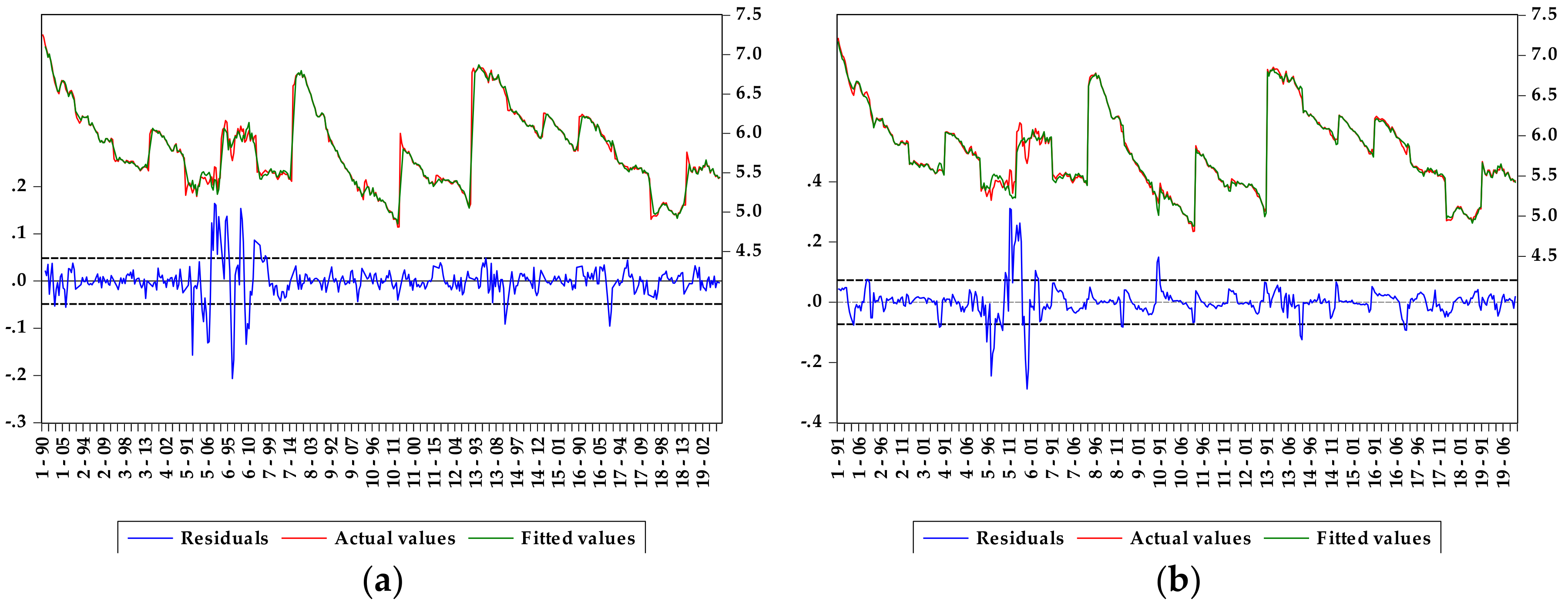
FECS and the second generation techniques, such as CIPS, were used for the other three variables. The results showed that the four variables were all non-stationary at levels but stationary at their first differences, which was consistent with some previous studies [12,22,39]. On this basis, three panel cointegration test approaches, Pedroni, Kao, and Fisher-type Johansen cointegration tests, were employed, suggesting that the long-term equilibrium among the analyzed variables existed, which is similar to the results of Dávalos [18] and Bölük and Mert [10], who investigated the related data of APEC and EU countries, respectively.
Next, DOLS and FMOLS techniques were applied to determine the long-term elasticity of CEI with respect to ECI, FECS, and PCGDP for panel, and the D–H panel causality test was then used to explore the existences and directions of the causal relationships among the variables, due to the endogeneity and heterogeneity possibly existing in the panel model. These empirical findings revealed that in the examined countries, energy factors affected development mode, and vice versa, and economic development level had a significant influence on energy factors and development mode.
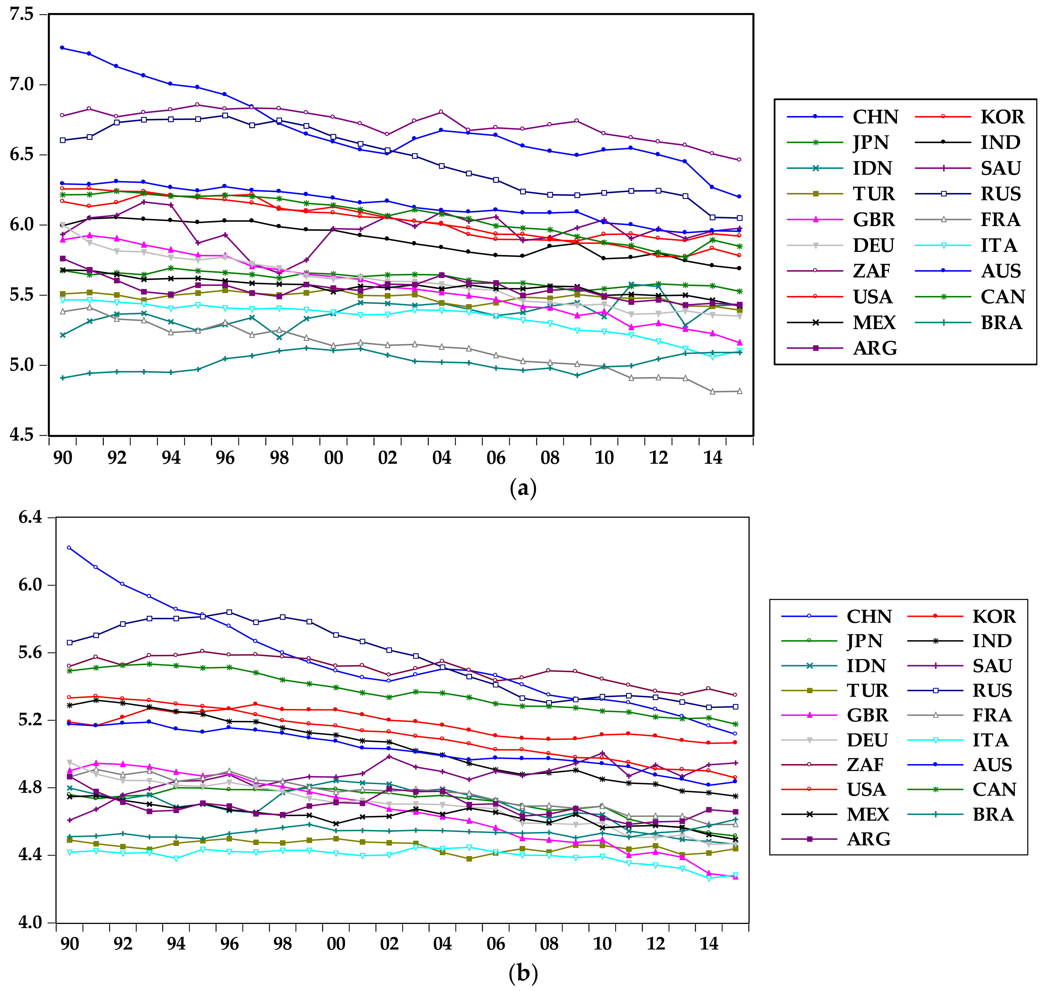
Furthermore, this paper estimated the long-run CEI elasticities with respect to ECI, FECS, and PCGDP for individuals applying the FMOLS approach, so as to explain the specific nexus among the four variables in the sample countries. The results showed that in most countries, ECI and FECS had significant and positive effects on CEI, indicating that the improvement of energy use efficiency and the optimization of energy use structure (indicating the reduction of fossil energy use) can help to decrease the CEI, in other words, to achieve a low-carbon development mode. In addition, PCGDP has positive influence on CEI in seven countries, while it has a negative influence in eight other countries, revealing that the current development modes in the seven countries will promote CO2 emissions continuously, which is unsustainable. For the remaining four countries, where the elasticities are not significant, governments should pay more attention to other factors affecting CEI, such as energy factors.
In line with the above empirical findings and discussions, some policy recommendations are proposed in this section. Firstly, considering the presence of CD issue in the panel, some international agreements, such as the Copenhagen Accord and Paris Agreement on Climate Change, are necessary, binding, and effective. Secondly, the improvement of energy use efficiency and the optimization of energy utilization structure can help to achieve a low-carbon development mode, as suggested by the results of FMOLS and DOLS for panel, having an important implication for the implementation of future policies on promoting the application of efficient energy use technologies and reducing the fossil energy consumption share. Finally, long-run elasticities estimation results for individuals showed that for different countries, energy factors and development level influence development mode differently. It can be inferred that there is no unified policy applied to all countries, and each country should formulate the policies that are consistent with its actual situation, so as to achieve a sustainable development mode with low carbon emissions.
Although this paper successfully explained the relationship between carbon intensity, economic development level, and energy factors (utilization efficiency and consumption structure) in G20 countries by employing the heterogeneous panel analysis approaches, there are still some limitations of this paper. Firstly, this paper used a semi-logarithmic model to explore the nonlinear relationship between the variables. In fact, the relationship between variables is not necessarily the form given in this paper. For example, it may be in the form of the environmental Kuznets curve (EKC). Therefore, exploring the relationship between variables under the EKC framework and comparing the results of EKC model with that in the logarithmic form can reveal the relationship between variables more deeply. Secondly, this article explored the factors that affect carbon intensity, including the level of economic development and energy factors. However, in the context of globalization, international trade will also have an impact on carbon intensity, which is not considered in this paper. In future research, international trade, investment, and other factors can be added in order to more fully reflect the impact mechanism of carbon intensity. Finally, the results of this study indicated that there were differences in the factors affecting carbon intensity among G20 countries, but the reasons for these differences were not further investigated. Therefore, in future studies, the more targeted time-series analysis techniques can be adopted for each country to explore its carbon intensity influencing factors, which can reflect the role each G20 country can play in the global carbon reduction process from a deeper level, instead of the role of the G20 mechanism described in this paper.

5.2. Discussions

The G20 includes large energy producing and consuming countries, as well as developing and developed countries. It can also play a coordinating role in the international energy organizations, such as IEA, OPEC, and so on, and the international economic organizations, such as the International Monetary Fund (IMF), the World Bank, the World Trade Organization (WTO), and the United Nations Conference on Trade and Development (UNCTAD). The G20 can largely overcome the major contradictions that have existed in the long-term global carbon emission reduction governance. Its membership and joint capabilities can greatly ease the contradiction and democratization among the subjects. Its strong coordination ability can integrate existing mechanisms and solve the problem of fragmentation of governance mechanisms, and its action ability and governance effectiveness can also effectively coordinate the differences in governance concepts.
The G20 has the willingness and ability to coordinate the interests of all parties in the world and mobilize all resources to implement global economic and carbon emission reduction governance. In the area of global carbon emission reduction governance that involves many overlapping issues, the G20 can effectively integrate carbon emission reduction with related issues such as energy, finance, and trade, showing that it is the only international governance mechanism that can play a global leading role today. Therefore, from the perspective of governance structure, governance capacity, and governance effectiveness, G20 can develop into the main coordination center for global carbon emission reduction governance.
In fact, the importance of G20 in the world has become increasingly prominent. For example, under the G20 framework, the issue of sustainable development in developing regions such as Africa has been emphasized, which has increased the global legitimacy of G20. At the same time, this effort has had a huge and decisive influence on the global governance system, that is, the UN Millennium Development Goals have been successfully upgraded to global sustainable development goals on schedule in 2015. In addition, G20 has been coordinating global climate governance policies among its members, which has accelerated the progress of the UN climate negotiations and finally reached the Paris Agreement. Therefore, some scholars believe that G20 will become the 21st century concert mechanism of powers.
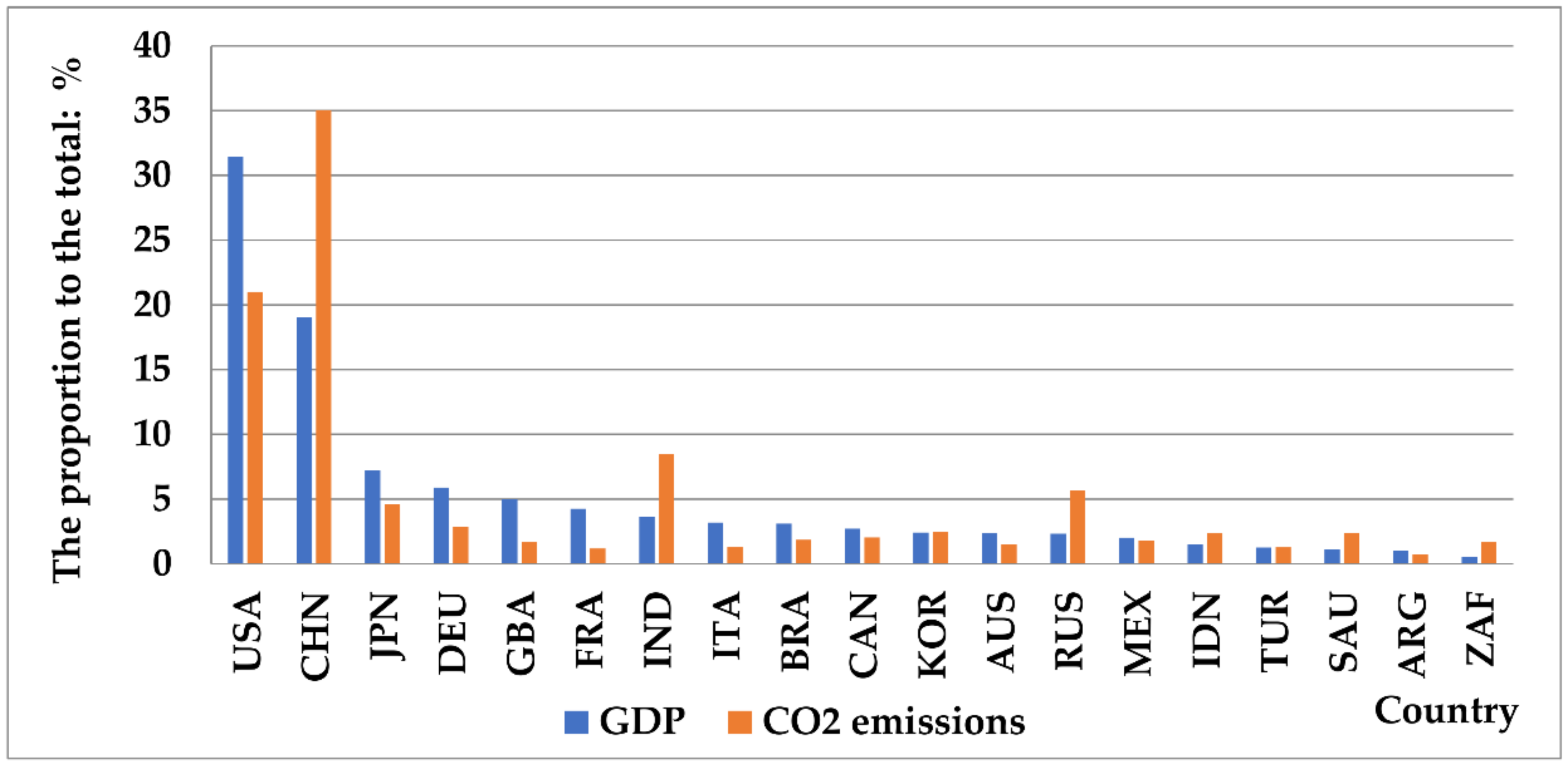
Therefore, this article focused on the G20 countries and examined the relationship among the G20 countries’ economic development mode, economic development level, and some energy factors, reflecting the main influencing factors and degree of impact of carbon emissions intensity in the overall G20 and each country, which is in line with the current trend of the G20 as a global carbon emission reduction governance coordination center. The research results of this paper show that there are serious energy and economic development imbalances among G20 countries, which make these countries have different and even conflicting interest needs and values in the process of jointly promoting global carbon emission reduction governance, resulting in mutual restraint or even offsetting of each other, which greatly affects the efficiency and effectiveness of global carbon emission reduction governance. In addition, G20 is mainly committed to responding to global economic governance issues that focus on finance, so it cannot be a single global carbon emission reduction governance mechanism, meaning that the status of carbon emission reduction issues in the G20 is fluctuating. Moreover, the G20 Summit is held alternately among member states. The host country has the priority of setting an annual meeting agenda, while other member states also have the power to shape the agenda according to their own preferences, which hinders the G20 from playing a leading role in global carbon emission reduction governance.

Author Contributions

H.L. and F.L. conceived and designed the research method used in this paper; X.Y. and D.S. collected the data; F.L. performed the empirical analysis and wrote the paper; S.F. provided valuable opinions during the revision and revised the paper specifically.

Funding

This research received no external funding.

Acknowledgments

Thanks are due to the North China Electric Power University Library for providing detailed reference for our research and to Li Bingkang for proofreading the language of this paper.

Conflicts of Interest

The authors declare no conflict of interest.

Appendix A

Figure A1. LCEI, LECI, LPCGDP and FECS in 19 G20 countries during 1990–2015. (a) LCEI in 19 G20 countries during 1990–2015; (b) LECI in 19 G20 countries during 1990–2015; (c) FECS in 19 G20 countries during 1990–2015; (d) LPCGDP in 19 G20 countries during 1990–2015.
Sustainability 10 02330 g0a1aSustainability 10 02330 g0a1b

Appendix B

Table A1. Estimation results of DOLS and FMOLS after adding time dummy variable.
VariableDOLSFMOLS
Coefficientt-StatisticCoefficientt-Statistic
LECI0.87632912.34442 (0.0000) ***0.85296417.85819 (0.0000) ***
FECS1.5077676.387706 (0.0000) ***1.60964811.55244 (0.0000) ***
LPCGDP−0.085034−1.726730 (0.0853) *−0.124515−4.169931 (0.0000) ***
T*LPCGDP−0.001999−1.480959 (0.1397)−0.000563−0.574549 (0.5659)
R-squared0.9952280.989042
Note: *, *** indicate the rejection of hull hypothesis at 10% and 1% significance level, respectively. T is time dummy variable valued by: T = 0 during 1990–2008 and T = 1 during 2009–2015. Numbers in parentheses are p-values.

Appendix C

Table A2. Descriptive statistics for the examined variables in panel and 19 G20 countries.
ObjectsVariablesMeanMedianMax.Min.Std.Dev.SkewnessKurtosisJBProb.
PanelLCEI5.80085.71557.25854.81010.49440.46792.708319.77830.0001 ***
LECI4.91744.82896.21964.26470.38500.63442.659435.52970.0000 ***
FECS0.80920.85651.00000.47940.1304−0.98133.001779.28540.0000 ***
LPCGDP9.850010.12210.8737.33070.8024−1.06133.550098.96790.0000 ***
ARGLCEI5.54365.54035.76085.42940.07690.77073.85673.36900.1855
LECI4.68974.68494.86684.58440.06710.72083.26872.32980.3120
FECS0.87900.88520.90660.83430.0182−0.96223.38564.17260.1241
LPCGDP9.65329.63939.89059.29040.1655−0.19552.20850.84430.6556
AUSLCEI6.14286.14056.30905.94420.1202−0.22671.79481.79640.4073
LECI5.02855.02255.18854.81510.1158−0.21271.88861.53430.4643
FECS0.93880.93900.95510.90890.0095−1.67786.918128.82900.0000 ***
LPCGDP10.48710.51010.68410.2360.1528−0.33841.68742.36270.3069
BRALCEI5.02025.01975.12214.90940.06490.05081.69821.84700.3971
LECI4.53744.53554.61254.49850.02610.90354.04934.73010.0939
FECS0.55140.54620.60000.51220.02540.20401.87161.55960.4585
LPCGDP9.40519.34899.63449.21230.13740.39551.77552.30190.3163
CANLCEI6.05806.09346.24145.76970.1512−0.44311.80712.39220.3024
LECI5.36815.36215.53265.17720.11650.03791.63532.02390.3635
FECS0.74600.74320.77120.72180.01360.36552.18531.29780.5226
LPCGDP10.52110.56210.66710.3130.1242−0.47661.67002.90060.2345
CHNLCEI6.69516.62507.25856.19820.27690.50272.50541.35990.5066
LECI5.54985.48056.21965.11760.29170.71052.65712.31460.3143
FECS0.82380.82120.88180.74830.0464−0.15921.49432.56610.2772
LPCGDP8.46188.41459.51577.33070.6750−0.00531.80041.55900.4586
DEULCEI5.59745.59766.00065.35050.18050.31292.20191.11430.5728
LECI4.69334.70374.95104.46650.1362−0.11872.02011.10120.5766
FECS0.83020.83230.87100.78940.02550.02231.68941.86290.3940
LPCGDP10.52610.52710.68710.3510.10210.04581.82181.51280.4694
FRALCEI5.12235.14005.41064.81010.1683−0.21182.18650.91130.6340
LECI4.76344.77894.90994.58240.1006−0.30141.93861.61430.4461
FECS0.52370.52750.58150.47940.02770.16902.67070.24120.8864
LPCGDP10.44610.47710.53910.2930.0899−0.55781.69503.19330.2026
GBRLCEI5.56125.55005.92445.16000.2295−0.00181.85921.40990.4941
LECI4.65724.66594.94534.27330.2121−0.21491.78551.79820.4069
FECS0.87030.87790.90650.74850.0338−2.35388.581857.76060.0000 ***
LPCGDP10.40710.46010.55910.1810.1322−0.54601.77672.91320.2330
IDNLCEI5.37385.36905.57615.19850.09090.18883.07760.16100.9227
LECI4.69104.71414.84214.46590.1134−0.62192.28792.22530.3287
FECS0.62490.62490.68490.53450.0391−0.70802.89302.18470.3354
LPCGDP8.81788.77519.24818.40680.23330.28312.13971.14900.5630
INDLCEI5.89325.88376.05175.68810.1184−0.11591.60172.17630.3368
LECI5.03635.04525.31904.75050.18650.02291.60882.09890.3501
FECS0.64950.64470.74780.53900.0606−0.11722.02211.09540.5783
LPCGDP7.99007.91238.65347.47060.37700.25191.78221.88150.3903
ITALCEI5.33325.37935.46555.05960.1161−1.02282.90814.54250.1032
LECI4.39654.41264.44844.26470.0471−1.47404.467511.7480.0028 ***
FECS0.89170.91370.93440.75320.0509−1.59154.303612.81730.0016 ***
LPCGDP10.46410.47010.56110.3460.0655−0.31761.92291.69390.4287
JPNLCEI5.61555.63735.69165.52610.0486−0.39131.89481.98660.3704
LECI4.71474.74874.80044.51500.0866−1.07272.93774.99090.0825
FECS0.83770.82420.94570.79240.04281.46084.021010.37570.0056 ***
LPCGDP10.44210.43810.54210.3240.0611−0.18012.00101.22160.5429
KORLCEI6.04026.03826.22185.88690.12540.11091.41852.76290.2512
LECI5.17535.18015.29535.06410.0760−0.00431.51092.40230.3008
FECS0.83980.83770.87740.80550.02130.25202.12131.11180.5736
LPCGDP10.00810.05610.4459.39990.3189−0.33161.89501.79940.4067
MEXLCEI5.56215.56345.67885.42230.0608−0.10062.95560.04600.9773
LECI4.63684.63994.75354.49350.0653−0.21222.59890.36930.8314
FECS0.88100.88020.91230.85990.01480.57582.59981.61050.4470
LPCGDP9.58619.59589.71059.43730.0848−0.28221.89951.65690.4367
RUSLCEI6.46896.51176.78006.04960.2430−0.20671.58912.34170.3101
LECI5.56025.59845.84005.27620.2107−0.07641.34442.99480.2237
FECS0.91180.90920.93390.87570.0133−0.70164.04753.32180.1900
LPCGDP9.79679.836410.1329.38580.2611−0.18091.53622.46310.2918
SAULCEI5.96105.97356.16395.65560.1200−0.74793.50012.69510.2599
LECI4.86484.87105.00554.60830.0870−1.18474.79929.58920.0083 ***
FECS0.99991.00001.00000.99980.0001−1.65954.956816.08190.0003 ***
LPCGDP10.58110.52610.82510.4220.13150.70682.02763.18890.2030
TURLCEI5.48315.49605.54475.39220.0385−0.77572.81772.64340.2667
LECI4.45414.45914.49944.37940.0319−0.51622.40341.54030.4629
FECS0.85880.86210.90570.81370.0318−0.05761.59962.13890.3432
LPCGDP9.56979.50439.87619.29180.19140.14601.64612.07810.3538
USALCEI6.02486.03766.25705.77310.1627−0.07471.69621.86580.3934
LECI5.11515.11825.34154.85850.1535−0.00981.71651.78500.4096
FECS0.85240.85660.86460.82300.0121−1.07802.89185.04880.0801
LPCGDP10.72210.75410.87310.5060.1203−0.56601.84982.82140.2440
ZAFLCEI6.71966.74006.85426.46190.1060−0.81182.83842.88430.2364
LECI5.49775.51255.60715.34760.0787−0.48532.11351.87210.3922
FECS0.86340.86480.88150.84240.0115−0.35821.88071.91340.3842
LPCGDP9.26579.23209.42829.10710.12130.16351.36343.01750.2212
Note: *** means the rejection of null hypothesis at 1% significance level.

Appendix D

Table A3. Leave-one-out analysis of the DOLS and FMOLS models of the other 17 G20 countries.
PanelVariableDOLSFMOLS
Coefficientt-StatisticCoefficientt-Statistic
Leave-ARG-OutLECI0.6598998.460966 (0.0000) ***0.5274826.991506 (0.0000) ***
FECS2.76142710.51585 (0.0000) ***3.07718313.26245 (0.0000) ***
LPCGDP−0.737773−35.92125 (0.0000) ***−0.707673−33.17158 (0.0000) ***
R-squared0.996968 0.990012
Leave-AUS-OutLECI0.6702658.500770 (0.0000) ***0.5367277.264670 (0.0000) ***
FECS2.78250810.58306 (0.0000) ***3.00572713.33246 (0.0000) ***
LPCGDP−0.733990−35.33294 (0.0000) ***−0.695898−33.57119 (0.0000) ***
R-squared0.996958 0.990136
Leave-BRA-OutLECI0.6282717.425294 (0.0000) ***0.5391716.769088 (0.0000) ***
FECS2.81701010.25864 (0.0000) ***3.03530412.77503 (0.0000) ***
LPCGDP−0.749380−32.31106 (0.0000) ***−0.700947−30.57646 (0.0000) ***
R-squared0.996734 0.989432
Leave-CAN-OutLECI0.6438988.020387 (0.0000) ***0.5132836.747444 (0.0000) ***
FECS2.70334710.02631 (0.0000) ***2.99444612.88254 (0.0000) ***
LPCGDP−0.735440−35.12468 (0.0000) ***−0.703431−33.29900 (0.0000) ***
R-squared0.996875 0.989797
Leave-DEU-OutLECI0.6943408.376073 (0.0000)***0.5312596.809521 (0.0000) ***
FECS2.90955410.35729 (0.0000)***3.06069612.84166 (0.0000) ***
LPCGDP−0.737110−35.45859 (0.0000)***−0.705874−33.13433 (0.0000) ***
R-squared0.996768 0.989244
Leave-FRA-OutLECI0.6477688.070161 (0.0000) ***0.5176726.783474 (0.0000) ***
FECS2.6695429.513515 (0.0000) ***2.98478112.58664 (0.0000) ***
LPCGDP−0.736301−35.30407 (0.0000) ***−0.704989−33.35527 (0.0000) ***
R-squared0.996514 0.988540
Leave-GBR-OutLECI0.6197047.089471 (0.0000) ***0.4974446.035261 (0.0000) ***
FECS2.80154610.38793 (0.0000) ***3.09210312.88390 (0.0000) ***
LPCGDP−0.744575−34.92636 (0.0000) ***−0.711626−33.23081 (0.0000) ***
R-squared0.996671 0.989279
Leave-IDN-OutLECI0.6251448.433421 (0.0000) ***0.4929226.633710 (0.0000) ***
FECS2.5230119.886191 (0.0000) ***2.89351712.64094 (0.0000) ***
LPCGDP−0.759849−38.33146 (0.0000) ***−0.719087−34.09006 (0.0000) ***
R-squared0.997238 0.990380
Leave-IND-OutLECI0.7607009.457737 (0.0000) ***0.5353286.772666 (0.0000)***
FECS2.1395317.062248 (0.0000) ***2.98693811.63276 (0.0000)***
LPCGDP−0.731923−36.67276 (0.0000) ***−0.706601−33.13597 (0.0000)***
R-squared0.996915 0.988974
Leave-ITA-OutLECI0.6620668.279109 (0.0000) ***0.5291626.934314 (0.0000) ***
FECS2.79931910.48835 (0.0000) ***3.18810812.41287 (0.0000) ***
LPCGDP−0.737770−35.17741 (0.0000) ***−0.709474−32.82144 (0.0000) ***
R-squared0.996689 0.989135
Leave-JPN-OutLECI0.5863687.261724 (0.0000) ***0.4761496.276325 (0.0000) ***
FECS3.16826211.02245 (0.0000) ***3.31710613.70062 (0.0000) ***
LPCGDP−0.757460−35.93471 (0.0000) ***−0.721348−34.16242 (0.0000) ***
R-squared0.996876 0.989854
Leave-KOR-OutLECI0.6375529.483746 (0.0000) ***0.4808937.293797 (0.0000) ***
FECS3.19783813.76297 (0.0000) ***3.37125716.46813 (0.0000) ***
LPCGDP−0.764759−42.84792 (0.0000) ***-0.738133−39.59840 (0.0000) ***
R-squared0.997737 0.991819
Leave-MEX-OutLECI0.6506248.094396 (0.0000) ***0.5236696.835581 (0.0000) ***
FECS2.79934510.41675 (0.0000) ***3.07352813.16321 (0.0000) ***
LPCGDP−0.742250−35.07831 (0.0000) ***−0.706862−33.02486 (0.0000) ***
R-squared0.996860 0.989679
Leave-RUS-OutLECI0.6110057.757693 (0.0000) ***0.4906766.635161 (0.0000) ***
FECS2.5928849.878923 (0.0000) ***2.84902712.80934 (0.0000) ***
LPCGDP−0.722741−35.07895 (0.0000) ***−0.689220−33.45115 (0.0000) ***
R-squared0.996575 0.989077
Leave-SAU-OutLECI0.6536177.283219 (0.0000) ***0.5443636.547296 (0.0000) ***
FECS2.79198810.24284 (0.0000) ***3.03654912.94825 (0.0000) ***
LPCGDP−0.741361−30.32340 (0.0000) ***−0.701453−29.76911 (0.0000) ***
R-squared0.996706 0.989237
Leave-TUR-OutLECI0.6980468.739909 (0.0000) ***0.5682327.386246 (0.0000) ***
FECS2.99433111.07747 (0.0000) ***3.16713013.67338 (0.0000) ***
LPCGDP−0.724400−33.90123 (0.0000) ***−0.691841−31.62318 (0.0000) ***
R-squared0.996977 0.989918
Leave-ZAF-OutLECI0.6495278.144548 (0.0000) ***0.5287106.968852 (0.0000) ***
FECS2.82166310.56422 (0.0000) ***3.07130913.36123 (0.0000) ***
LPCGDP−0.736715−35.22945 (0.0000) ***−0.701673−33.16205 (0.0000) ***
R-squared0.996583 0.988891
Notes: *** denotes that the coefficients are significant at the 1% significance level. Numbers in parentheses are p-values.

References

  1. Kraft, J.; Kraft, A. On the relationship between energy and GNP. Energy Dev. 1978, 3, 401–403. [Google Scholar]
  2. Akarca, A.T.; Long, T.V. On the relationship between energy and GNP: A reexamination. J. Energy Dev. 1980, 5, 326–331. [Google Scholar]
  3. Akinlo, A.E. Energy consumption and economic growth: Evidence from 11 Sub-Sahara African countries. Energy Econ. 2008, 30, 2391–2400. [Google Scholar] [CrossRef]
  4. Belke, A.; Dobnik, F.; Dreger, C. Energy consumption and economic growth: New insights into the cointegration relationship. Energy Econ. 2011, 33, 782–789. [Google Scholar] [CrossRef] [Green Version]
  5. Apergis, N.; Payne, J.E. Energy consumption and economic growth in Central America: Evidence from a panel cointegration and error correction model. Energy Econ. 2009, 31, 211–216. [Google Scholar] [CrossRef]
  6. Ouedraogo, N.S. Energy consumption and economic growth: Evidence from the economic community of West African States. Energy Econ. 2013, 36, 637–647. [Google Scholar] [CrossRef]
  7. Arouri, M.E.H.; Youssef, A.B.; M’henni, H.; Rault, C. Energy consumption, economic growth and CO2 emissions in Middle East and North African countries. Energy Policy 2012, 45, 342–349. [Google Scholar] [CrossRef] [Green Version]
  8. Kasman, A.; Duman, Y.S. CO2 emissions, economic growth, energy consumption, trade and urbanization in new EU member and candidate countries: A panel data analysis. Econ. Model. 2015, 44, 97–103. [Google Scholar] [CrossRef]
  9. Magazzino, C. The relationship between real GDP, CO2 emissions, and energy use in the GCC countries: A time series approach. Cogent Econ. Financ. 2016, 4, 1–20. [Google Scholar] [CrossRef]
  10. Lotfalipour, M.R.; Falahi, M.A.; Ashena, M. Economic growth, CO2 emissions, and fossil fuels consumption in Iran. Energy 2010, 35, 5115–5120. [Google Scholar] [CrossRef]
  11. Sebri, M.; Ben-Salha, O. On the causal dynamics between economic growth, renewable energy consumption, CO2 emissions and trade openness: Fresh evidence from BRICS countries. Renew. Sustain. Energy Rev. 2014, 39, 14–23. [Google Scholar] [CrossRef]
  12. Jebli, M.B.; Youssef, S.B.; Ozturk, I. Testing environmental Kuznets curve hypothesis: The role of renewable and non-renewable energy consumption and trade in OECD countries. Ecol. Indic. 2016, 60, 824–831. [Google Scholar] [CrossRef]
  13. Bhattacharya, M.; Paramati, S.R.; Ozturk, I.; Bhattacharya, S. The effect of renewable energy consumption on economic growth: Evidence from top 38 countries. Appl. Energy 2016, 162, 733–741. [Google Scholar] [CrossRef]
  14. Zhang, M.; Bai, C.; Zhou, M. Decomposition analysis for assessing the progress in decoupling relationship between coal consumption and economic growth in China. Resour. Conserv. Recycl. 2018, 129, 454–462. [Google Scholar] [CrossRef]
  15. Apergis, N.; Payne, J.E. Natural gas consumption and economic growth: A panel investigation of 67 countries. Appl. Energy 2010, 87, 2759–2763. [Google Scholar] [CrossRef]
  16. Marques, A.C.; Fuinhas, J.A.; Nunes, A.R. Electricity generation mix and economic growth: What role is being played by nuclear sources and carbon dioxide emissions in France? Energy Policy 2016, 92, 7–19. [Google Scholar] [CrossRef]
  17. Salahuddin, M.; Gow, J.; Ozturk, I. Is the long-run relationship between economic growth, electricity consumption, carbon dioxide emissions and financial development in Gulf Cooperation Council Countries robust? Renew. Sustain. Energy Rev. 2015, 51, 317–326. [Google Scholar] [CrossRef] [Green Version]
  18. Dávalos, J. Sustainable Economic Growth: An Empirical Study for the Asia-Pacific Economic Cooperation Forum. Int. J. Energy Econ. Policy 2016, 6, 594–601. [Google Scholar]
  19. Jorgenson, A.K. Economic development and the carbon intensity of human well-being. Nat. Clim. Chang. 2014, 4, 186–189. [Google Scholar] [CrossRef]
  20. Alshehry, A.S.; Belloumi, M. Energy consumption, carbon dioxide emissions and economic growth: The case of Saudi Arabia. Renew. Sustain. Energy Rev. 2015, 41, 237–247. [Google Scholar] [CrossRef]
  21. Li, H.; Li, B.; Lu, H. Carbon Dioxide Emissions, Economic Growth, and Selected Types of Fossil Energy Consumption in China: Empirical Evidence from 1965 to 2015. Sustainability 2017, 9, 697. [Google Scholar]
  22. Dogan, E.; Ozturk, I. The influence of renewable and non-renewable energy consumption and real income on CO2 emissions in the USA: Evidence from structural break tests. Environ. Sci. Pollut. Res. 2017, 24, 10846–10854. [Google Scholar] [CrossRef] [PubMed]
  23. Lu, H.; Campbell, D.E.; Sagisaka, M.; Ren, H. Interactions among energy consumption, economic development and greenhouse gas emissions in Japan after World War II. Renew. Sustain. Energy Rev. 2016, 54, 1060–1072. [Google Scholar] [CrossRef]
  24. Granger, C.W.J. Investigating causal relations by econometric models and cross-spectral methods. Econom. J. Econom. Soc. 1969, 37, 424–438. [Google Scholar] [CrossRef]
  25. Granger, C.W.J. Testing for causality: A personal viewpoint. J. Econ. Dyn. Control 1980, 2, 329–352. [Google Scholar] [CrossRef]
  26. Granger, C.W.J. Some recent development in a concept of causality. J. Econom. 1988, 39, 199–211. [Google Scholar] [CrossRef]
  27. Habib, S. Revising the Empirical Linkage between Renewable Energy Consumption and Economic Growth in Tunisia: Evidence from ARDL Model. Int. J. Sustain. Econ. Manag. 2017, 1303–1316. [Google Scholar] [CrossRef]
  28. Streimikiene, D.; Kasperowicz, R. Review of economic growth and energy consumption: A panel cointegration analysis for EU countries. Renew. Sustain. Energy Rev. 2016, 59, 1545–1549. [Google Scholar] [CrossRef]
  29. Saboori, B.; Sulaiman, J. CO2 emissions, energy consumption and economic growth in Association of Southeast Asian Nations (ASEAN) countries: A cointegration approach. Energy 2013, 55, 813–822. [Google Scholar] [CrossRef]
  30. Pesaran, M.H. A simple panel unit root test in the presence of cross-section dependence. J. Appl. Econom. 2007, 22, 265–312. [Google Scholar] [CrossRef] [Green Version]
  31. Pesaran, M.H. General Diagnostic Tests for Cross Section Dependence in Panels. Available online: https://papers.ssrn.com/sol3/papers.cfm?abstract_id=572504 (accessed on 4 August 2004).
  32. Breitung, J. The local power of some unit root tests for panel data. In Nonstationary Panels, Panel Cointegration, and Dynamic Panels; Emerald Group Publishing Limited: Bingley, UK, 2001; pp. 161–177. [Google Scholar]
  33. Levin, A.; Lin, C.F.; Chu, C.S.J. Unit root tests in panel data: Asymptotic and finite-sample properties. J. Econom. 2002, 108, 1–24. [Google Scholar] [CrossRef]
  34. Im, K.S.; Pesaran, M.H.; Shin, Y. Testing for unit roots in heterogeneous panels. J. Econom. 2003, 115, 53–74. [Google Scholar] [CrossRef]
  35. Maddala, G.S.; Wu, S. A comparative study of unit root tests with panel data and a new simple test. Oxf. Bull. Econ. Stat. 1999, 61, 631–652. [Google Scholar] [CrossRef]
  36. Pedroni, P. Critical Values for Cointegration Tests in Heterogeneous Panels with Multiple Regressors. Oxf. Bull. Econ. Stat. 1999, 61, 653–670. [Google Scholar] [CrossRef]
  37. Pedroni, P. Panel Cointegration: A Symptotic and Finite Sample Properties of Pooled Time Series Tests with an Application to the PPP Hypothesis. Econ. Theory 2004, 20, 597–625. [Google Scholar] [CrossRef]
  38. Zhao, H.; Zhao, H.; Han, X.; He, Z.; Guo, S. Economic Growth, Electricity Consumption, Labor Force and Capital Input: A More Comprehensive Analysis on North China Using Panel Data. Energies 2016, 9, 891. [Google Scholar] [CrossRef]
  39. Salahuddin, M.; Alam, K.; Ozturk, I. The effects of Internet usage and economic growth on CO2 emissions in OECD countries: A panel investigation. Renew. Sustain. Energy Rev. 2016, 62, 1226–1235. [Google Scholar] [CrossRef]
  40. Destek, M.A.; Balli, E.; Manga, M. The Relationship between CO2 Emission, Energy Consumption, Urbanization and Trade Openness for Selected CEECs. Res. World Econ. 2016, 7, 52–58. [Google Scholar] [CrossRef]
  41. Liobikienė, G.; Butkus, M. Environmental Kuznets Curve of greenhouse gas emissions including technological progress and substitution effects. Energy 2017, 135, 237–248. [Google Scholar] [CrossRef]
  42. Kaika, D.; Zervas, E. The Environmental Kuznets Curve (EKC) theory—Part, A.: Concept, causes and the CO2 emissions case. Energy Policy 2013, 62, 1392–1402. [Google Scholar] [CrossRef]
  43. Azam, M.; Khan, A.Q. Testing the Environmental Kuznets Curve hypothesis: A comparative empirical study for low, lower middle, upper middle and high income countries. Renew. Sustain. Energy Rev. 2016, 63, 556–567. [Google Scholar] [CrossRef]
  44. Kais, S.; Sami, H. An econometric study of the impact of economic growth and energy use on carbon missions: Panel data evidence from fifty-eight countries. Renew. Sustain. Energy Rev. 2016, 59, 1101–1110. [Google Scholar] [CrossRef]
  45. Bilgili, F.; Kocak, E.; Bulut, U. The dynamic impact of renewable energy consumption on CO2 emissions: A revised Environmental Kuznets Curve approach. Renew. Sustain. Energy Rev. 2016, 54, 838–845. [Google Scholar] [CrossRef]
  46. Jarque, C.M.; Bera, A.K. Efficient tests for normality, homoscedasticity and serial independence of regression residuals. Econ. Lett. 1980, 6, 255–259. [Google Scholar] [CrossRef]
  47. Kao, C.; Chiang, M.H. On the estimation and inference of a cointegrated regression in panel data. In Nonstationary Panels, Panel Cointegration, and Dynamic Panels; Emerald Group Publishing Limited: Bingley, UK, 2001; pp. 179–222. [Google Scholar]
  48. Pedroni, P. Fully modified OLS for heterogeneous cointegrated panels. In Nonstationary Panels, Panel Cointegration, and Dynamic Panels; Emerald Group Publishing Limited: Bingley, UK, 2001; pp. 93–130. [Google Scholar]
  49. Mark, N.C.; Sul, D. Cointegration vector estimation by panel DOLS and long-run money demand. Oxf. Bull. Econ. Stat. 2003, 65, 655–680. [Google Scholar] [CrossRef]
  50. Perron, P.; Ng, S. Useful modifications to some unit root tests with dependent errors and their local asymptotic properties. Rev. Econ. Stud. 1996, 63, 435–463. [Google Scholar] [CrossRef]
  51. Breitung, J. A parametric approach to the estimation of cointegration vectors in panel data. Econom. Rev. 2005, 24, 151–173. [Google Scholar] [CrossRef]
  52. Dumitrescu, E.I.; Hurlin, C. Testing for Granger non-causality in heterogeneous panels. Econ. Model. 2012, 29, 1450–1460. [Google Scholar] [CrossRef] [Green Version]
  53. Kao, C. Spurious regression and residual-based tests for cointegration in panel data. J. Econom. 1999, 90, 1–44. [Google Scholar] [CrossRef]
  54. Fukunaga, K.; Hummels, D.M. Leave-one-out procedures for nonparametric error estimates. IEEE Trans. Pattern Anal. Mach. Intell. 1989, 11, 421–423. [Google Scholar] [CrossRef]
  55. Kearns, M.; Ron, D. Algorithmic stability and sanity-check bounds for leave-one-out cross-validation. Neural Comput. 1999, 11, 1427–1453. [Google Scholar] [CrossRef] [PubMed]
  56. Refaeilzadeh, P.; Tang, L.; Liu, H. Cross-validation. In Encyclopedia of Database Systems; Springer: Boston, MA, USA, 2009; pp. 532–538. [Google Scholar]
  57. Han, V. Trump’s Promise: Withdrawing from the Paris Climate Agreement. Environ. Claims J. 2017, 29, 337–349. [Google Scholar] [CrossRef]
  58. Böehringer, C.; Rutherford, T.F. US Withdrawal from the Paris Agreement: Economic Implications and Carbon-Tariff Conflicts. Discussion Paper 2017-89. Cambridge, Mass.: Harvard Project on Climate Agreements, August 2017. Available online: https://www.belfercenter.org/sites/default/files/files/publication/dp89_bohringer-rutherford.pdf (accessed on 31 August 2017).
  59. Donald, P. Withdrawing from the Paris climate agreement hurts the US. Nature 2017, 2, 17145. [Google Scholar]
  60. Sohu News. China’s Ministry of Foreign Affairs: All Parties Should Jointly Cherish and Safeguard the Hard-Won Fruits of the Paris Agreement. Available online: http://www.sohu.com/a/145533884_157267 (accessed on 2 June 2017).
Figure 1. Actual, fitted, and residual graph of the DOLS and FMOLS models. (a) Graph of DOLS model and (b) graph of the FMOLS model.
Sustainability 10 02330 g001
Figure 2. The proportions of gross domestic product (GDP) and CO2 emissions of 19 Group of Twenty (G20) countries to the total in 2015.
Sustainability 10 02330 g002
Table 1. Literature review on energy-economic-emission linkages.
StudyMethodologyPeriodObjectFindings
Apergis, N. and Payne, J.E. [5]Panel cointegration and error correction model1980–20046 Central American CountriesBoth short-run and long-run causality from energy consumption to economic growth.
Ouedraogo, N.S. [6]Panel cointegration techniques and dynamic error correction model1980–200815 African countriesCausality from gross domestic product (GDP) to energy consumption in the short-run, and from energy consumption to GDP in the long-run.
Magazzino, C. [9]Structural breaks analysis, cointegration test, ARDL, T–Y causality test1960–20136 GCC countriesKuwait, Oman, and Qatar show a growth hypothesis, while no long-run relation has been discovered in Saudi Arabia.
Sebri, M. et al., [11]ARDL bounds testing approach and VECM1971–2010BRICS countriesLong-run equilibrium relationships among the competing variables, and feedback hypothesis.
Dávalos, J. [18]Three EKC models, panel econometric methods1992–2012APEC countriesEKC is held under Model 1 and 3, but not for Model 2.
Li, H. et al., [21]Time series econometric model accounting for structural breaks1965–2015ChinaGDP–coal use and CO2 emissions–coal use causality, and unidirectional causality from GDP to CO2 emissions.
Dogan, E. and
Ozturk, I. [22]
Time series econometric model with structural breaks, EKC model1980–2014The United StatesEKC hypothesis is not valid for the USA, and the increases in renewable energy consumption mitigate environmental degradation.
Lu, H. et al. [23]An integrated suite of energy, emergy and economic indices1946–2011JapanComplicated interactions among energy consumption, economic development, and the potential impact of green house gas (GHG) emissions.
Habib, S. [27]C–D production function and ARDL model1980–2011TunisiaThe feedback hypothesis in long term and the conservation hypothesis in short-run
Streimikiene, D., et al. [28]Panel econometric models involving DOLS and FMOLS1995–201218 EU countriesEconomic growth, energy consumption and gross fixed capital are cointegrated for the panels.
Saboori, B. and Sulaiman, J. [29]ARDL model, Granger test based on VECM, and EKC model1971–20095 ASEAN countriesEKC was held in Singapore and Thailand, and bi-directional causality between CO2 emissions and energy consumption is found.
Zhao, H., et al. [38]C–D production function, panel data analysis methods1995–20146 provinces in North ChinaElectricity use-real GDP causality in six provinces except Hebei, capital input-economic growth and labor force input-economic growth causalities except Beijing and Hebei.
Salahuddin, M., et al. [39]Panel cointegration test, pooled mean group (PMG) estimates1991–201231 OECD countriesInternet usage and economic growth has no significant short-run and long-run effects on CO2 emissions.
Destek, M.A., et al. [40]EKC model, FMOLS, panel Granger test based on VECM1991–201110 CEECsEKC hypothesis, and bidirectional causalities between CO2 emissions and real GDP and between real GDP and energy consumption.
Table 2. Correlations for the panel data set (p values in parentheses). LCEI—log CO2 emissions intensity; LECI—log energy consumption intensity; FECS—fossil energy consumption share; LPCGDP—log GDP per capita.
LCEILECIFECSLPCGDP
LCEI10.9052 (0.0000) ***0.4599 (0.0000) ***−0.2326 (0.0000) ***
LECI 10.1289 (0.0041) ***−0.2652 (0.0000) ***
FECS 10.3636 (0.0000) ***
LPCGDP 1
Note: *** denotes statistical significance at 1% level.
Table 3. Pesaran cross-sectional dependence (CD) test results.
VariableLCEILECILPCGDPFECSOverall
Pesaran CD test33.60734.66556.920−1.4466.176
Prob.0.0000 ***0.0000 ***0.0000 ***0.14810.0000 ***
Notes: *** indicates the rejection of null hypothesis at the 1% significance level.
Table 4. Panel unit roots results. CIPS—cross-sectional augmented IPS.
First Generation Panel Unit Root TestSecond Generation Panel Unit Root Test
LLCADF-FisherCIPS TestLCEILECILPCGDP
FECS2.503147.1603Level−1.976−2.063−1.972
ΔFECS−14.3403 **246.766 ***1st diff.−4.818 **-4.872 **−3.328 **
Notes: **, *** Denote the rejection of null hypothesis the 5% and 1% significance levels, respectively.
Table 5. Results of panel cointegration test.
Pedroni Residual Cointegration Test
Test StatisticsStatisticsProb.
Panel v-Statistic1.8452070.0325 **
Panel rho-Statistic−1.1507390.1249
Panel PP-Statistic−4.9301860.0000 ***
Panel ADF-Statistic−4.4812150.0000 ***
Group rho-Statistic0.9494830.8288
Group PP-Statistic−3.8410090.0000 ***
Group ADF-Statistic−6.8375770.0000 ***
Kao Cointegration Test
ADF−5.8475760.0000 ***
Fisher-Type Johansen Cointegration Test
Hypothesized No. of CE(s)Fisher Statistic
Trace testProb.Max-Eigen TestProb.
None204.60.0000 ***142.50.0000 ***
At most 195.190.0000 ***75.020.0003 ***
At most 249.260.104451.940.0654 *
At most 328.020.882028.020.8820
Notes: *, **, and *** denote the rejections of null hypothesis at 10%, 5%, and 1% significance levels, respectively. CE means cointegration equation.
Table 6. Estimation results of the DOLS and FMOLS models for panel (Dependent variable: LCEI).
VariableDOLSFMOLS
Coefficientt-StatisticCoefficientt-Statistic
LECI0.91808013.35154 (0.0000) ***0.86031518.51310 (0.0000) ***
FECS1.6023577.171070 (0.0000) ***1.62879311.91828 (0.0000) ***
LPCGDP−0.080282−1.808599 (0.0715) *−0.131898−4.566282 (0.0000) ***
R-squared0.9955190.988977
Notes: *, *** denote that the coefficients are significant at the significance levels of 10% and 1%, respectively. Numbers in parentheses are p-values.
Table 7. Autocorrelation test of residual diagnostic based on the Q-statistic.
ModelLag123456789101112
DOLSQ-stat.2.013.544.335.055.636.727.558.568.848.929.7410.42
p-value0.15630.17030.22800.28220.34390.34750.37390.38080.45220.53970.55390.5792
FMOLSQ-stat.2.473.585.056.518.429.9410.4711.5313.4615.1117.0217.68
p-value0.11600.16700.16820.16420.13460.12720.1635 0.17340.14290.12810.10730.1258
Table 8. Leave-one-out analysis of the DOLS and FMOLS models of United States (USA) and China (CHN).
PanelVariableDOLSFMOLS
Coefficientt-StatisticCoefficientt-Statistic
Leave-USA-OutLECI0.6524307.914612 (0.0000) ***0.5022626.377249 (0.0000) ***
FECS2.78103110.28128 (0.0000) ***3.02929512.93956 (0.0000) ***
LPCGDP−0.741046−35.19387 (0.0000) ***−0.709874−33.34560 (0.0000) ***
R-squared0.996800 0.989600
Leave-CHN-OutLECI0.6424647.835912(0.0000) ***0.6203838.641818 (0.0000) ***
FECS2.75943810.31361(0.0000) ***2.68553012.50117 (0.0000) ***
LPCGDP−0.744864−34.98348(0.0000) ***−0.723521−37.21875 (0.0000) ***
R-squared0.996309 0.990106
Notes: *** denotes that the coefficients are significant at the 1% significance level. Numbers in parentheses are p-values.
Table 9. Lag order selection criteria of panel causality test.
LagLRFPEAICSCHQ
0NA   8.60 × 10 6 −0.312658−0.267807−0.294791
15986.932 1.54 × 10 13 *−17.98447−17.65323−17.89513
249.42437 *   1.69 × 10 13 −18.15248 *−17.76021 *−17.89609
355.27703   1.82 × 10 13 −18.05690−17.56941−17.92020 *
462.23067   1.56 × 10 13 −18.13552−17.37304−17.83177
Notes: * indicates lag order selected by the criterion. LR means sequential modified LR test statistic (each test at 5% level), FPE means final prediction error, AIC means Akaike information criterion. SC means Schwarz information criterion, and HQ means Hannan–Quinn information criterion.
Table 10. Results of heterogeneous panel causality test.
Null HypothesisLag = 2Lag = 1Lag = 3
Zbar-Stat.Prob.Zbar-Stat.Prob.Zbar-Stat.Prob.
LECI does not homogeneously cause LCEI3.474890.0005 ***3.501970.0005 ***1.908240.0564
LCEI does not homogeneously cause LECI4.596330.0000 ***4.593950.0000 ***3.969500.0000 ***
FECS does not homogeneously cause LCEI2.939100.0033 ***4.567340.0000 ***1.007290.3138
LCEI does not homogeneously cause FECS3.565790.0004 ***2.916810.0035 ***3.432470.0006 ***
LPCGP does not homogeneously cause LCEI4.040470.0001 ***5.800430.0000 ***1.560220.1187
LCEI does not homogeneously cause LPCGP1.125200.26053.058440.0022 ***-0.234740.8144
FECS does not homogeneously cause LECI4.609600.0000 ***7.286360.0000 ***3.395160.0007 ***
LECI does not homogeneously cause FECS3.388480.0007 ***3.472420.0005 ***2.808480.0050 ***
LPCGP does not homogeneously cause LECI8.118770.0000 ***7.044590.0000 ***6.129260.0000 ***
LECI does not homogeneously cause LPCGP0.960720.33673.211290.0013 ***1.109370.2673
LPCGP does not homogeneously cause FECS2.293700.0218 **2.044920.0409 **1.558390.1191
FECS does not homogeneously cause LPCGP1.778910.0753 *5.176220.0000 ***0.464740.6421
Notes: *, **, *** mean the rejections of null hypothesis at the significance levels of 10%, 5%, and 1%, respectively.
Table 11. Estimation result of the FMOLS models for individuals (Dependent variable: LCEI).
VariableLECIFECSLPCGDPR2Ad-R2
ARG1.0539 (0.0000) ***1.7812 (0.0008) ***−0.2160 (0.2197)0.89100.8811
AUS1.0436 (0.0000) ***−1.3107 (0.0009) ***0.4680 (0.0000) ***0.98430.9829
BRA0.3894 (0.1637)0.9897 (0.0803) *0.6761 (0.0826) *0.91040.9022
CAN1.2437 (0.0000) ***3.7337 (0.0000) ***−0.7892 (0.0000) ***0.98140.9797
CHN1.1797 (0.0000) ***1.9129 (0.0209) **−0.3245 (0.1952)0.98310.9815
DEU0.8512 (0.0000) ***2.6935 (0.0008) ***−0.1436 (0.0156) **0.98670.9855
FRA1.0949 (0.0000) ***3.0086 (0.0000) ***−0.4223 (0.0000) ***0.99620.9958
GBR1.0096 (0.0000) ***−0.0679 (0.3034)0.3508 (0.1091)0.98380.9823
IDN0.1042 (0.5609)−0.6335 (0.5576)1.2768 (0.0013) ***0.17540.1004
IND0.7330 (0.0000) ***−0.1330 (0.1342)0.7827 (0.0031) ***0.96420.9609
ITA-0.3748 (0.4382)0.9479 (0.0014) ***1.3684 (0.0121) **0.92810.9216
JPN0.9093 (0.0000) ***0.9600 (0.0005) ***0.1188 (0.2704)0.87970.8687
KOR1.2416 (0.0000) ***2.3748 (0.0000) ***−0.5378 (0.0001) ***0.95030.9458
MEX0.7948 (0.0000) ***−1.3811 (0.0268) **0.6902 (0.0021) ***0.93020.9239
RUS0.9981 (0.0000) ***3.4661 (0.0000) ***−0.4966 (0.0000) ***0.99430.9938
SAU1.1869 (0.0505) *−2643.5 (0.0447) **574.04 (0.0444) **0.18150.1071
TUR1.1209 (0.0000) ***−0.0377 (0.9079)0.1174 (0.5462)0.75780.7358
USA1.0447 (0.0000) ***3.7751 (0.0002) ***−0.5772 (0.0015) ***0.99820.9964
ZAF1.4893 (0.0000) ***2.6764 (0.0414) **−0.8484 (0.0457) **0.94730.8946
Notes: R2 and Ad-R2 mean the R-squared and adjusted R-squared of the model. *, **, and *** denote that the coefficients are significant at the significance levels of 10%, 5%, and 1%, respectively, and numbers in parentheses are p-values.

