4.1. Data Preprocessing
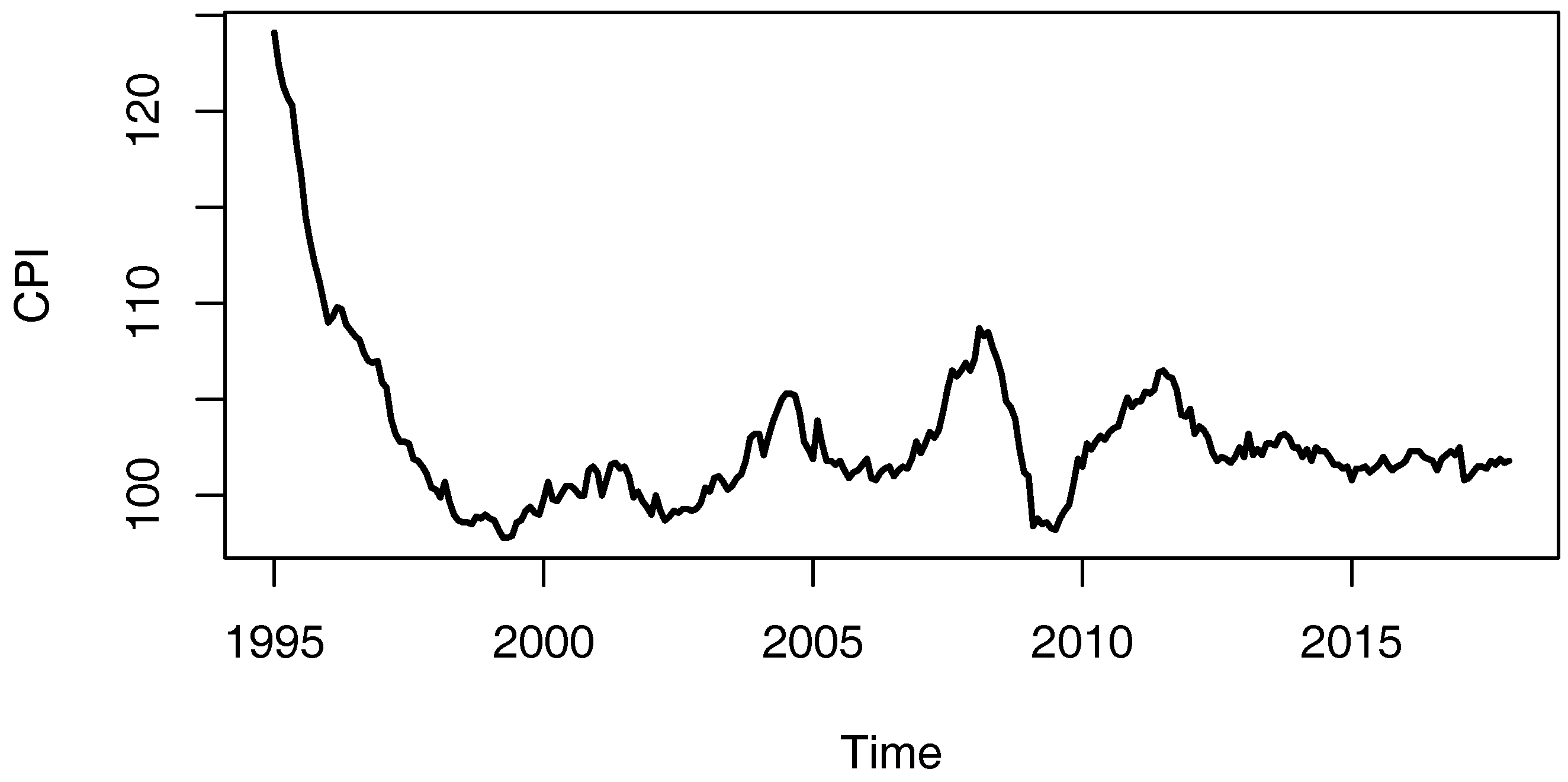
In this paper, inflation is measured in terms of the Consumer Price Index (CPI). The growth rate of CPI can be regarded as a proxy for the inflation rate. In particular, we use the monthly CPI data of China from Jan. 1995 to December 2017, with a total of 276 observations denoted as
. The data is displayed in
Figure 1, showing that the CPI is quite large in the beginning of this period and drops down slowly. The inflation rate has been relatively stable at a level around 2% since 2012, which indicates that the development of the economy of China has stepped into the stage of “New Normal”. Intuitively, the underlying inflation process may change since the beginning of the “New Normal” period.
In practice, we take the logarithm of the raw CPI data, and check the stationarity of the log-CPI data, at significance level 0.05. The result of the Phillips-Perron unit root test shows that the log-CPI data is nonstationary (with
p-value 0.1494), but the first order difference of the log-CPI is stationary (with
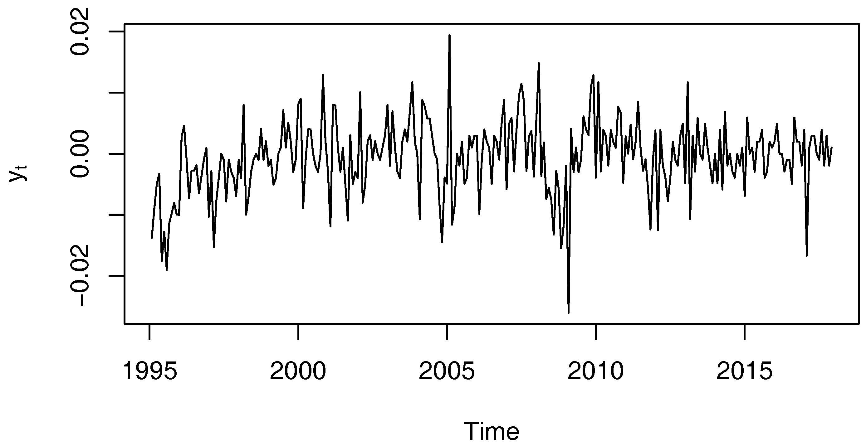
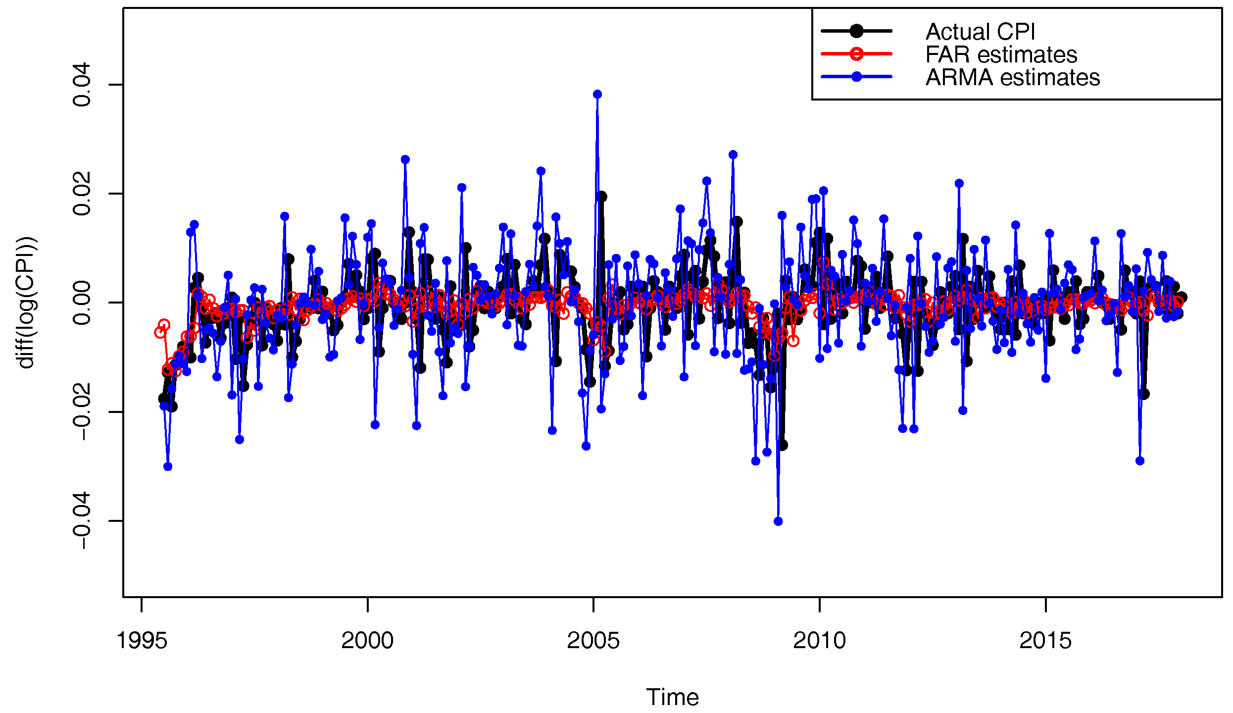
p-value 0). Therefore, the following analysis is based on the first order difference of the log-CPI denoted as
The plot of
is shown in
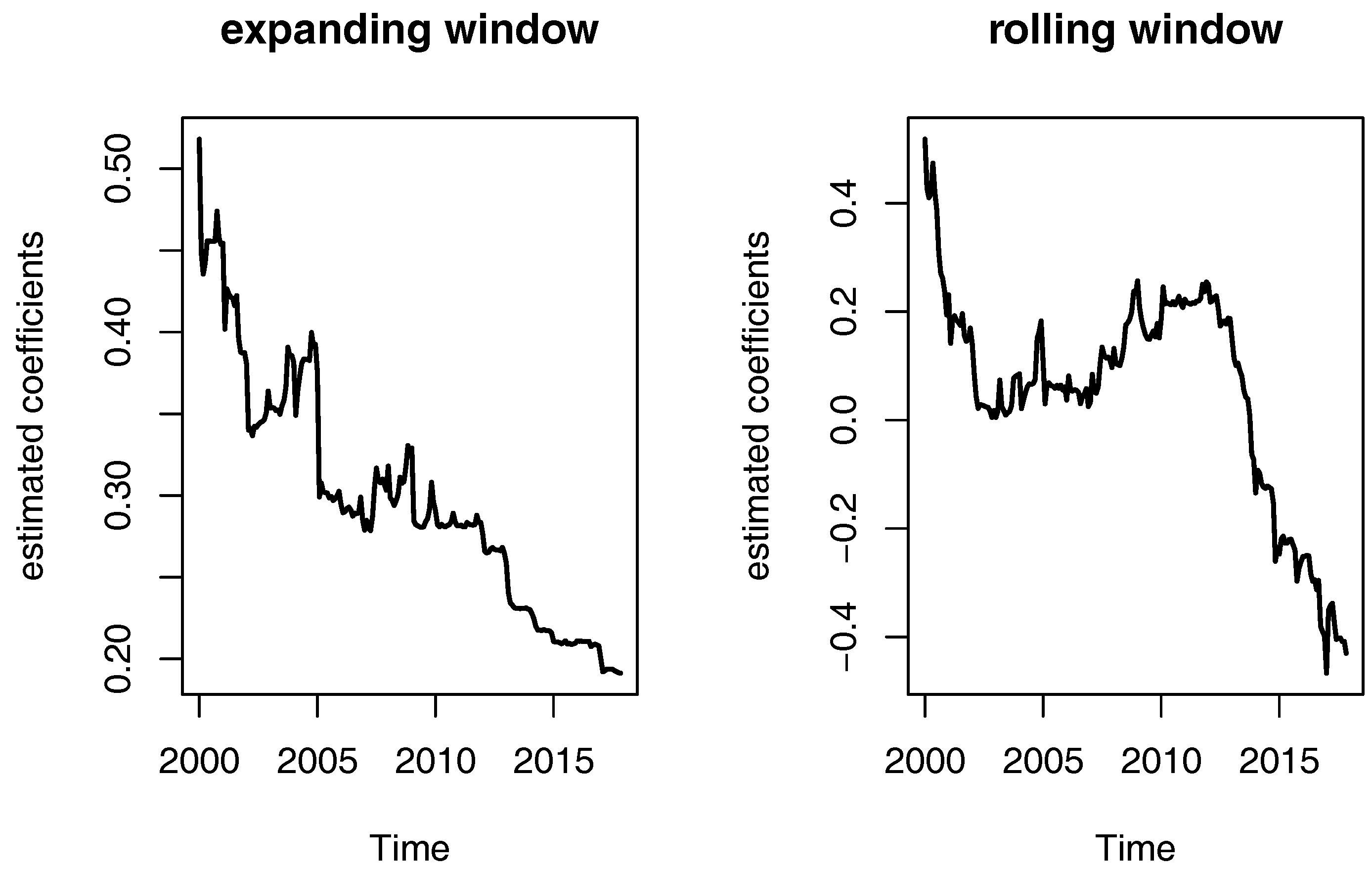
Figure 2. Parameter instability is also observed in our analysis of the data. We build an AR(1) model
and estimate the AR coefficient
on an expanding window basis and rolling window basis with a 60 window-width. These estimates are plotted in
Figure 3. It can be seen that the estimates of
are quite variable. In conclusion, a non-linear FAR(
) model with time-varying coefficients is more reasonable and flexible than the linear ARMA model.
4.2. In-Sample Fit Analysis
We first use the FAR(
) model (
2) to fit
given in (
15). Based on the AIC values, we have
. Then
. For a given threshold lag
d, the FAR(
) model is estimated by the B-splines method. To construct the B-spline basis, the degree of the B-spline basis, the number and locations of the knots need to be determined. We consider different choices of the degree
K and the number of interior knots
M, i.e.,
and
. For different values of
, the locations of the knots
,
are set to be the
sample quantiles (
) of
. The B-spline basis can be calculated according to (
5) and (
6), and is then used to estimate the FAR(
) model by (
9). We use the AIC criterion to determine the value of
.
Table 4 reports the AIC values for different combinations of
, showing that
leads to the smallest value of AIC. Therefore, we use
as the threshold variable.
and
implies that the computational complexity is not large. The only internal knot is the median of
, while the boundary knots are
and
, respectively. Thus, the resulting augmented vector of knots is (
,
,
,
,
, 0.0194).
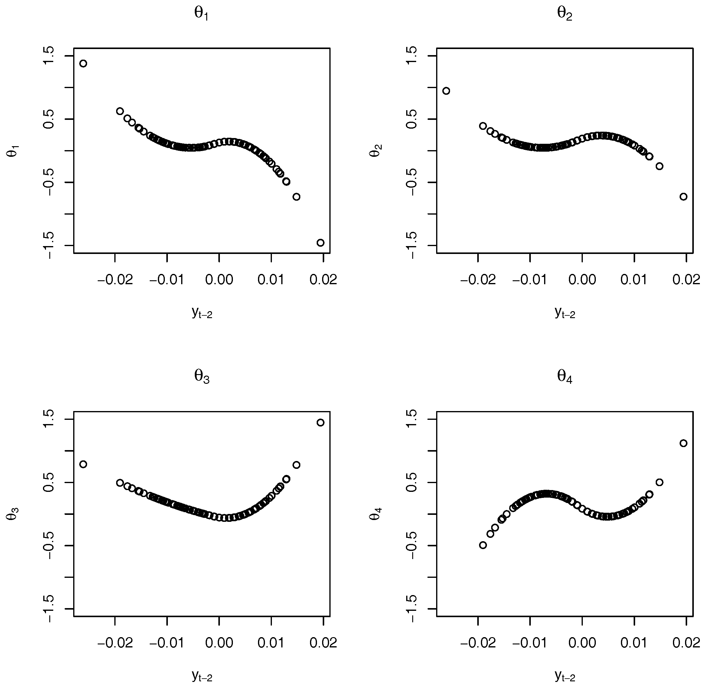
The estimated FAR(4,2) model is
where the estimated coefficients are
, where
are given in
Table 5.
Based on the B-spline estimation results in
Table 5, we plot the estimated functional coefficients of the FAR(4,2) model (16) in
Figure 4. The fitted first order differenced monthly log-CPI
can be recursively obtained by (
16). The Ljung-Box test shows that the residuals
is a white noise sequence, indicating that the FAR(4,2) model provides a satisfactory model fitting. By substituting
into (15), we obtain the fitted CPI
.
We also fit
by an ARMA(
) model, where
. The order
p and
q are determined by the AIC criterion, which gives
. The estimated model is
where
are residuals. Also, the residuals of model (17) are white noise, implying a satisfactory model fitting.
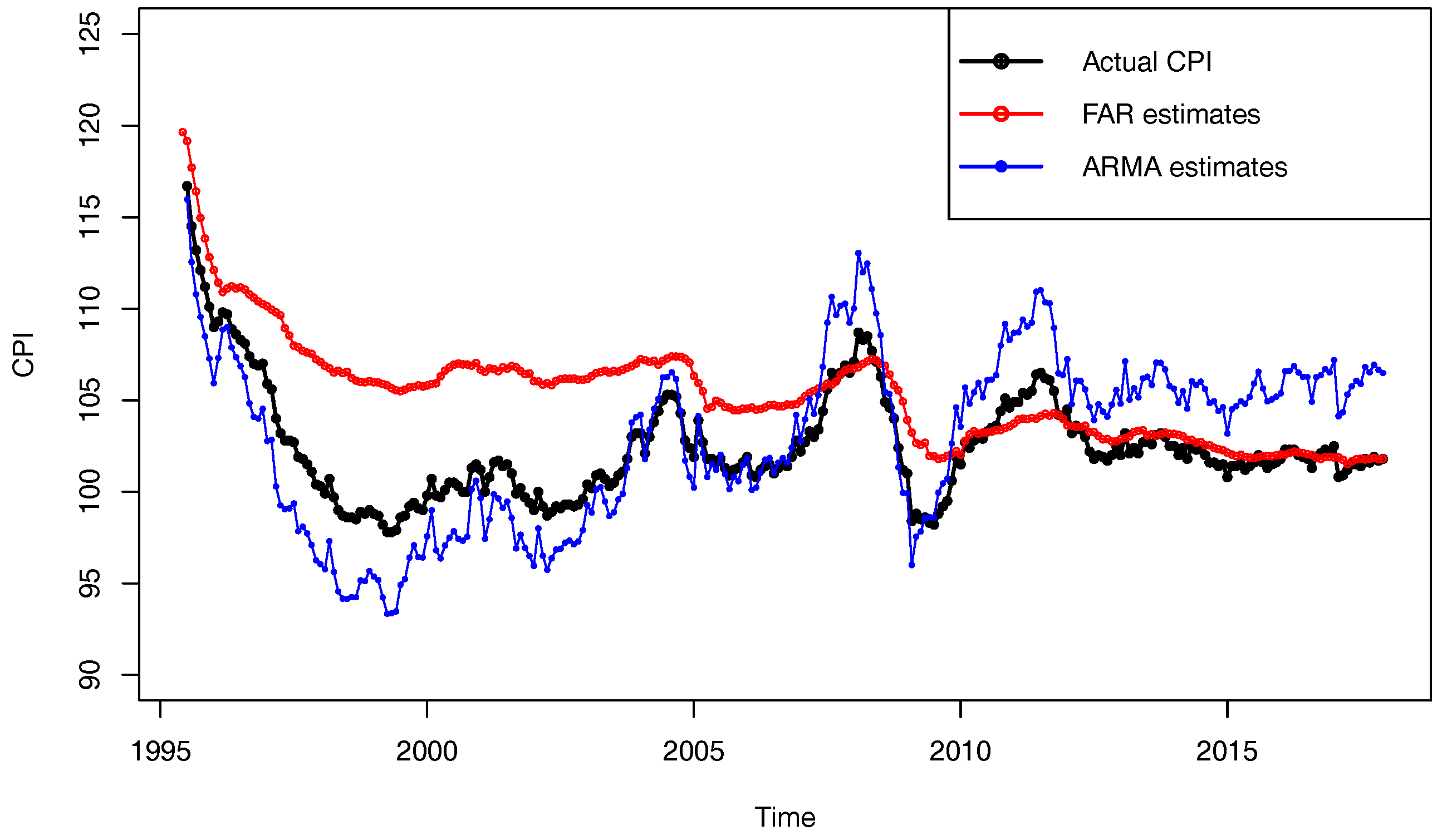
Figure 5 and
Figure 6 display
and
given by the estimated FAR(4,2) and ARMA(5,5) models, respectively. From
Figure 6, both the FAR(4,2) and the ARMA(5,5) describe the main characteristic of data quite well. In particular, they capture the three falling and rising processes of the inflation since 1995. Intuitively, the fitted ARMA(5,5) is more fluctuated, meaning that the model overestimates the peak and underestimates the trough, while the fitted FAR(4,2) model is more smoothing, i.e., the FAR(4,2) model underestimates the peak and overestimates the trough. Thus, it is expected that the ARMA(5,5) model fit the CPI data better during the fluctuating period, while the FAR(4,2) model performs better during the stable period. From
Figure 6, the inflation rate during 1995 to 2011 fluctuates heavily, and the fitted CPI by using the ARMA(5,5) model is closer to the real CPI than that given by the FAR(4,2) model. However, for the period from 2012 to 2017, the inflation rate is quite stable around the level of 2%, and the FAR(4,2) model performs better.
We compare the fitting performance of the FAR(4,2) model and the ARMA(5,5) model for
by using mean absolute errors (MAE) and RMSE defined as
and
The definitions of MAE and RMSE for
are similar and thus are omitted. Furthermore, to compare predictive accuracy, we employ the Diebold and Mariano test (denoted as DM test hereafter) proposed in Diebold and Mariano (1995) [
29], based on the corresponding MAE and RMSE. We only introduce the DM test based on the MAE for simplicity. Define the forecasting error of
as
and the loss function
. Based on
, the forecasting loss difference between ARMA and FAR is
. Here, the null hypothesis is that the ARMA model has equal predictive accuracy as the FAR model, which is equivalent to
. Let
, then the DM statistic is given by
where
is a consistent estimate of the standard deviation of
. The alternative can be set as the forecast of FAR is more accurate than that of ARMA. The procedure proceeds as follows. First, we calculate DM test statistic and the two-sided
p-value based on the limiting standard normal distribution. Then if the value of the test statistic is positive (negative), the one-sided
p-value is just one half of the two-sided
p-value (one minus one half of the two-sided
p-value). Similarly, if the alternative is that the forecast of ARMA is more accurate than that of FAR, and the value of the test statistic is positive (negative), the one-sided
p-value is one minus a half of the two-sided
p-value (one half of the two-sided
p-value).
In addition, we divide the in-sample forecasts into two halves: the first half ranges from January 1995 to September 2006 and the second half ranges from October 2006 to December 2017. The two-sided testing results are given in
Table 6. We first discuss the forecast of
. With the full sample, the MAE and RMSE of ARMA(5,5) model are almost the same as those of FAR(4,2) model for fitting
. The scenario is similar for the first period data and the second period data. This fact is in line with the DM test results, which shows that in most cases, the fitting accuracies of the two models are similar under the 5% significance level.
Then we consider the results for . For the full sample, the MAE of ARMA(5,5) is 15.8% smaller than those of FAR(4,2) model for fitting . This improvement increases to 58.19% with the first period data, which can be also verified by the larger absolute values of the DM statistic. The DM test result implies that the ARMA(5,5) model provides better fitting accuracies than the FAR(4,2) model. However, for the more stable second period data, the MAE of ARMA(5,5) is three times of that of FAR(4,2) model. This superiority can be also verified by the DM test. Therefore, the FAR(4,2) model has better fitting accuracy for more stable data. Similar conclusions can be obtained based on RMSE.
Combining the previous analysis, it is expected that the FAR model will provide more accurate prediction for when China are stepping into the “New Normal” stage.
4.3. Out of Sample Forecast
From the in-sample analysis, the predictive performance of each model is not the same for periods before and in the stage of “New Normal”. Compared to the in-sample fitting, the out-of-sample forecasting of a model is more important, since precise forecasts of the inflation rate are crucial for economic agents (e.g., investors, consumers) as well as for economic policy decision makers. In particular, we are interested in the inflation rate for the period of “New Normal”. Thus, we divide the whole sample into two parts: the first part covers data from January 1995 to October 2013, and the second part covers data from November 2013 to December 2017. We use the rolling window method to obtain the future CPI value. That is, when the forecast proceeds, the estimation window rolls forward by adding one new data and dropping the most distant data. In this way, the size of the estimation window remains the same. The one-step-ahead forecast is implemented based on the estimated FAR(4,2) model (16) and the ARMA(5,5) model (17). To get an
h-step-ahead forecast (
), we can iteratively implement one-step-ahead forecast
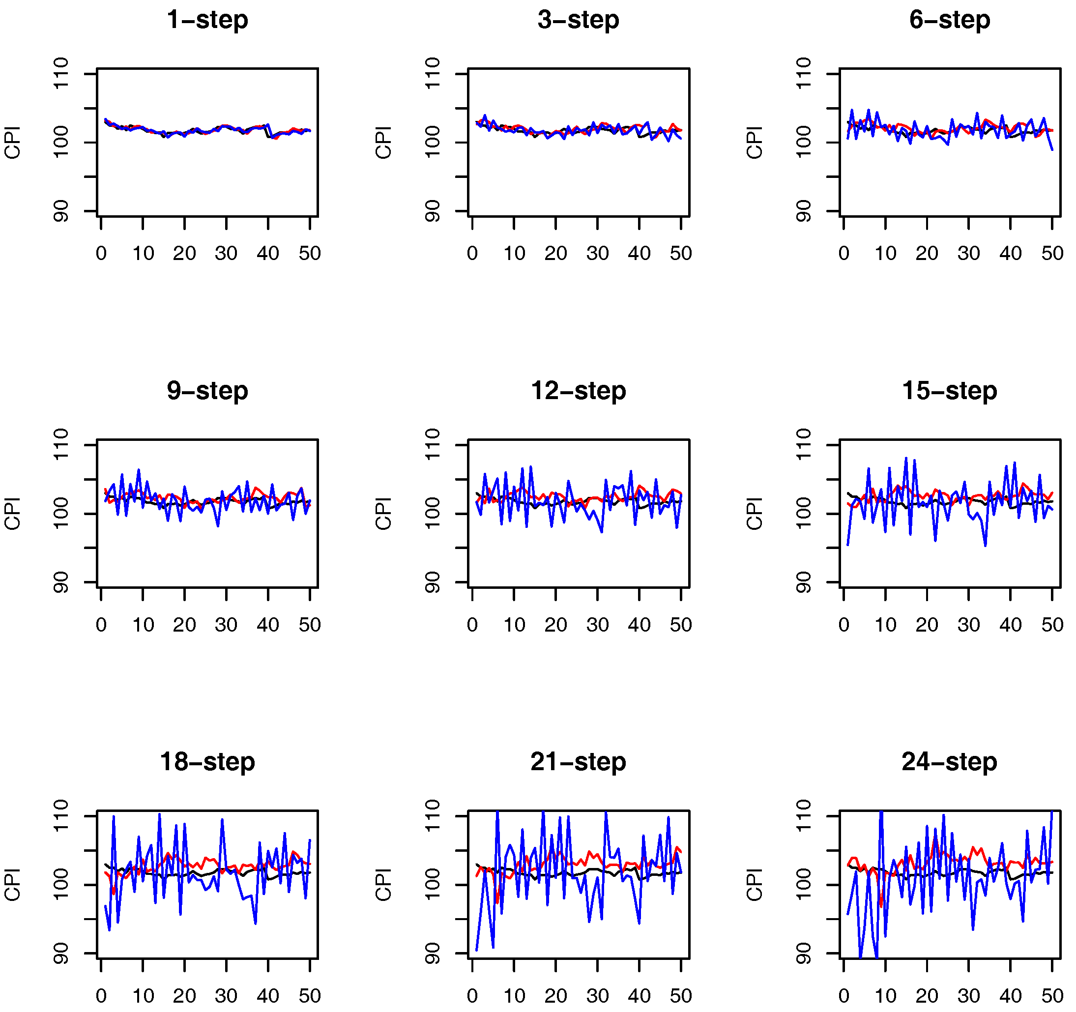
h times as given in (12). In the following, we consider different values of forecast horizons
. The forecasting results are shown in
Figure 7.
The figure shows that the forecasts based on the FAR(4,2) model are more smoothing, while the forecasts based on the ARMA(5,5) model are more fluctuated. Since the true CPI data in the forecasting period are stable, the FAR(4,2) model provide more accurate forecasts. It is also shown that as h increases, the forecasts for both models become more fluctuated and less accurate.
To evaluate the forecasting accuracy, we use the forecasting MAE and RMSE defined as
and
respectively, where
is the true CPI, and
is the
h-step-ahead forecast of CPI,
N is the total number of forecasts. We also conduct the DM test for comparison. In
Table 7, we report the MAE, the RMSE, the DM statistic and the
p-value with alternative hypothesis that the two models have different predictive accuracies. The forecast horizon is fixed at
. It can be observed that at short horizon levels (i.e.,
), the MAE and RMSE of the two models are comparable. When the horizon level becomes large (i.e.,
), the MAE and RMSE of FAR(4,2) model are lower than those of ARMA(5,5) model. Moreover, as the horizon level
h increases, the improvement of FAR(4,2) model becomes larger. This phenomenon is also detected by the DM test. Specifically, at 5% significance level, the FAR(4,2) model outperforms the ARMA(5,5) model for
, while the predictive accuracies of the two models are similar for
. This fact implies that the FAR model is better for moderate and long-term inflation rate forecasting and is comparable to ARMA model for short-term inflation rate forecasting.


