Influence Factors and Regression Model of Urban Housing Prices Based on Internet Open Access Data

Abstract

With the commercialization of housing and the deepening of urbanization in China, housing prices are having increasing influence on the land market, and thus indirectly affecting urban development. As various spatial features of an urban housing property directly affect its price, the study of this connection has significance for urban planning. The present study uses mainly open internet data of housing prices, supplemented by other data sources, to identify the spatial features of housing prices and the influence factors in a case study city, Wuhan. Methods employed in the study include the hedonic linear regression model, the geographically weighted regression (GWR) model and the artificial neural network (ANN) model, etc. Progress is made in the following two aspects: first, when calculating the influence factors, hierarchical values for accessibility variables of certain public facilities are used instead of simple Euclidean distance and the results shows a better model fit; second, the ANN model shows the best fit in the study, and while the three models all show respective strengths, the combined use of all models offers the possibility of a more comprehensive analysis of the influence factors of housing prices.

1. Research Background

With the commercialization of housing and the deepening of urbanization in China, housing prices show an increasing influence on the land market, and thus affect urban planning and urban development [1]. The urban spatial features of a housing property are closely associated to its price [2]. Therefore, in the urban planning discipline which directly guides the spatial development of cities, attention should be given to the study of the spatial features and the mechanism of how they influence housing price.

In studies on housing price and its influence factors, the hedonic model proposed by Rosen is the most commonly used approach [3]. The influence factors in early studies include the location feature, neighborhood feature and architectural feature [4]; later studies incorporate other factors such as accessibility [5], land-use planning [6]; and more recent studies further introduce external environmental factors such as natural scenery [7], block size [8], wind power generator [9] into the model to analyze their influence on housing prices.

The hedonic method mainly uses the regression analysis to build a function model of housing prices and various influence factors, and then discusses the effect of each factor on a house price. However, stemming from economic theory, the hedonic method does not choose a specific functional form nor specific influence factors. Therefore, researchers have to conduct multiple experiments in order to select the factor variables and corresponding processing functions with a better fit in the regression analysis, leading to the fact that different factors [10] and processing functions [11] are proposed in various studies. Many scholars find that, in the hedonic regression model, housing price does not exhibit a simple linear relationship with its influence factors [12]. Hence, logarithmic and semi-logarithmic functions are used to process the original variables [13,14]. However, errors brought about by non-linear conversion still cannot be avoided (the more the variables, the greater the error) [15]. Therefore, some researchers attempt to analyze the relationship between the influence factors and house price from a non-linear perspective [16,17], such as building the neural network model, to predict housing price. The model is proven to offer a better fit than the regular linear regression model.

In studies based on the hedonic model, one assumption is that all influence factors have a constant influence regardless of their different geospatial locations, while in reality, factors such as neighborhood feature and accessibility usually have a strong autocorrelation. According to the first law of geography, everything is interconnected and this link grows stronger with closer proximity [18]. On top of these, some scholars proposed the geographically weighted regression (GWR) model [19,20] in which the parameters and their weights can be adjust locally in accordance with their spatial locations. To date, this model has been widely applied in many fields such as geography [21], economics [22], environmental science [23] and epidemiology [24]. Various works of research on housing price show that in studies of the same influence factor, results using the GWR model show a better fit than the simple hedonic model [25,26]. The spatial analysis capability of the GWR model makes it more suitable for studies on the impact of accessibility and the layout of transportation facilities on housing price [27,28,29]. In addition, the sample data obtained at different time intervals also affect the fitting results. Therefore, time is introduced into the regular GWR model as a characteristic variable, which further enhances the model’s adaptability to time sequence data [30,31,32].

In early studies, samples mainly come from survey data or statistical reports. They are usually limited in number and lack timeliness. Therefore, the research results can hardly be used in urban policy-making due to the lag in time. In recent years, network open data have been gradually applied in GWR-based studies [33,34]. Such data sources significantly increase the number of samples with improved accuracy and timeliness [35].

Although extensively used in studies of the housing markets in many countries, the hedonic model and the research findings cannot be directly applied in the Chinese context due to cultural and social differences [36]. The present study represents an endeavor in research methodology, using mainly open internet data of housing price, supplemented by other data sources such as location-based service (LBS), point of interest (POI) and urban planning data, to select the influence factors of housing price and further compare multiple regression models and analyze the relationships between the influence factors and housing price in the case study city Wuhan.

2. Data Acquisition and Processing

2.1. Data Categories

(1) Housing Price-Related Data

Various housing property websites in China offer information of the name, average unit price, location and other information of commercial housing properties such as the age, floor area ratio (FAR), and the price change over the years. In addition, with improved quality of internet map services provided by companies such as Baidu and Gaode, the locations of these housing properties can now be acquired with enhanced accuracy and compatibility. The major source of the price data is the Anjuke website, supplemented by Fangtianxia and Lianjia websites. In the study, the sales prices of 6397 residential properties are acquired through data crawling and the data of the age of these properties are acquired through multiple source websites. According to the Anjuke website, its housing price data come from two major sources, i.e., user-posted data and offline survey data. These data are then processed by a specific algorithm which takes into account both the posted selling price and final transaction price. By comparison with those of other sources, the data from the Anjuke website is more accurate in relation to the actual price in the Chinese housing market and, thus, is used in the present study as the unit price of various housing properties in the study period.

(2) Point of Interest Data

As a result of urban informatization, various public service facilities such as primary and secondary schools, hospitals and bus stops can be located on internet map services as Point of Interest (POI), which offers the name, spatial latitude and longitude coordinates and other attributes. The major sources of POI of the present study are the Baidu map and 8684 bus information services, data of public facilities are acquired through web crawling, such as primary and secondary schools, hospitals, supermarkets and bus stops (including the number of bus routes and subway stations).

(3) Location-based Service Data

Location-based Service (LBS) data is mainly generated by mobile end devices such as mobile phones and can reflect the spatial distribution and movement trajectory of urban residents at a specific time. Two types of LBS data are used in the present study: the first type is mobile phone call data, which is used to calculate and classify population density by analyzing the time points, frequency and spatial location of base stations of phone calls over a study period of one month; base stations with the highest frequency of phone calls during work time and non-work time (off-time) are identified as the work and residence base stations of the user, respectively; furthermore, the spatial units in which these base stations are located are used for population analysis. Mobile phone data is used instead of data from the population census or statistical yearbook because the latter tend to have a long time lag and lack spatial division, and thus could not satisfy the demand of timeliness and accuracy of spatial unit division for this study. The second type of data is acquired by crawling the Dianping.com website which is a Chinese website for user-generated rating and comments of restaurants (similar to yelp.com), including the spatial location of restaurants and the corresponding number of reviews, used to assess the prosperity of urban commercial service facilities.

(4) Urban Planning and Internet Map Data

Based on relevant urban planning maps of Wuhan, the spatial layout of the artery roads including the inner ring road and the third ring road of the city and the spatial units divided by urban roads are obtained. Combined with land-use maps, and Google Map aerial images, data of natural elements such as waterways, lakes and parks are obtained, including their boundaries and areas.

2.2. Data Pre-processing

(1) Coordinate calibration: as Google Map aerial images use the wgs84 world coordinate system, while road and land-use maps of the Wuhan urban planning are based on the Beijing Geodetic Coordinate System 54, maps in the present study are uniformly calibrated based on the wgs84 system to facilitate subsequent analysis. In addition, as other data acquired by web crawling such as the spatial location of residential properties, the POI data, etc. are all based on shifted coordinates, they are also calibrated and restored to the wgs84 coordinate system. Finally, layers of different elements are superimposed on the aerial map, including point elements such as the location of properties, POIs, restaurant locations and number of reviews, line elements such as the road network, as well as surface elements such as urban greens and water areas.

(2) Division of spatial units: to facilitate the spatial analysis of housing prices from an urban perspective, the division of spatial units is defined as the carrier of various variables. The functional areas divided by urban roads are used as the basic units in the present study, on the basis of which, conversion and calculation of statistics of various types are carried out. Housing prices of residential properties and the associated location data are imported into ArcGIS as point elements. To facilitate subsequent analysis at the land-unit scale and to produce relevant planning strategies, these point elements are then numbered and associated to specific spatial units. Furthermore, the average price of each unit of land is calculated. Numbers of mobile phone users are assigned to different land units through the location data of base stations, and then the population of each land unit is calculated based on the telecom operator’s market share. Then, population density is obtained by dividing the population by the land area of each unit.

3. Methodology

3.1. Selection of Influence Factors of Housing Price

From the planning perspective, five types of influence factors are selected, including location feature, architectural and neighborhood feature, public facility feature, traffic accessibility feature and natural environment feature, to analyze their impact on housing price. Specifically, two types of distance values are used for the factors: the first is the commonly used spatial Euclidean distance, the second is the classified and hierarchical distance value calculated based on kernel density. As there are usually overlapping areas or differences in the service of public facilities, the simple spatial Euclidean distance approach means ignoring all these factors while the kernel density approach takes into account not only the interaction between spatial points, but also specific parameters of factors as different weights. For example, the service capacity (and its hierarchy) is used as a parameter which reflects the different spatial areas of influence of facilities at different hierarchies.

(1) Location Feature

Simply put, location feature means that the closer a place is to the city center (commercial center), the better its location is. In the present study, two location parameters are selected. One is the simple spatial distance to the inner city ring road. Through the neighborhood analysis, the distances from the inner ring to various spatial units are calculated as the values of location feature. Negative values are taken inside the inner ring and positive values outside the inner ring. The other is the hierarchical values of the major commercial centers in the city. As these centers do not have physical boundaries and have different influences, simple spatial distance is not used, but rather kernel density analysis based on the restaurants’ distribution and number of user comments acquired from the dianping.com website is used to calculate the hierarchical influences of various commercial centers (Figure 1) as another location feature value. Spatial distribution of restaurants is used as a substitute variable for commericial centers in kernel density analysis, as a more important commercial center attracts higher density of restaurants and a greater number of consumers. Therefore, restaurants weighted by the number of comments generates a diagram such as Figure 1 which represents the influence hierarchy of the commercial centers that the restaurants are located in.

(2) Architectural and Neighborhood Feature

Age of the property, i.e., 2017 minus the year of completion, is the only data used as an architectural feature in the present study. In addition, housing properties are classified as to whether they are villas or not, while only non-villas are used for the calculation. From the planning point of view, the green coverage of most residential properties is between 30% and 35%, while the floor area ratio is also decided by the regulatory planning system. Since, most of the data on the websites are provided by developers instead of by actual surveying, the data are not used in the study as important architectural features. In terms of neighborhood feature, two factors, namely population density and the number of supermarkets in the spatial unit, are used. The calculation of population density is a relative value as described in Section 2.2. Property management fee, as studied by various research works, is not incorporated in the present study as a factor because its relationship with housing price in the Chinese market is yet to be identified, and often the property management fee is decided by housing price. Besides, property management fees charged by certain welfare housing properties or collectively built properties are not priced by the market and the data are also difficult to collect.

(3) Public Facility as an Influence Factor

Three types of commonly used public facilities, such as Grade A Class Three hospitals, middle schools and primary schools, are used in the study as influence factors. As Grade A Class Three hospitals are considered city-level services, geometric distances to them are used as parameters. For primary- and middle-school factors, relative values are calculated and weighted by whether they are key schools, and through kernel density analysis, the results are used as the parameter of factors in accordance with the service hierarchies of various spatial units.

(4) Traffic Accessibility Feature

Two types of traffic data are used in the study, bus and subway data. Among them, bus data are relative hierarchical values by overlapping the spatial distribution of bus stations and kernel density analysis of the weights of bus lines at each bus stop. However, subway stations are calculated using the spatial geometric distance to the nearest station.

(5) Natural Environment Feature

Three types of factors are considered as features of the natural environment: river view, water area and urban public green space. Among them, the river view factor is presented as the spatial distance from each spatial unit to the Yangtze River or the Han River, while water area and urban public green space are calculated and graded by overlapping their spatial distribution and areas, and then are analyzed and graded by kernel density. Thus, the parameters for respective factors are obtained.

The spatial units generated in the present study are represented as polygon elements in ArcGIS. The housing price and influence factor parameters in each spatial unit have been preprocessed, eliminating values that may lead to significant errors in model calculation, such as zero values and dummy elements. The result includes 1565 spatial units and 13 corresponding influence factors.

3.2. Hedonic Model Regression Analysis Based on SPSS

Housing prices and the 13 factors in five categories are coded and preliminarily analyzed as in

Table 1. Housing prices and influence factors.

	N	Minimum	Maximum	Mean	Std. Deviation
Housing Price (Price)	1565	5061	71,880	18,825.060	5677.224
Number of supermarkets (Market)	1565	0	103	21.870	17.227
Distance to inner ring (InnerRing)	1565	56	14,344	3773.12	3223.489
Population density (Population)	1565	1	292,047	22,291.020	29,693.297
Age of building (Age)	1565	−3	37	14.138	6.369
Distance to river (River)	1565	0	15,955	3188.369	3105.678
Water area (Water)	1565	1	24	4.185	3.917
Commercial center (Commercial)	1565	1	49	6.021	8.588
Distance to metro station (Metro)	1565	52.955	7294.524	1345.166	1354.341
Bus (Bus)	1565	1	30	12.013	6.567
Hospital (Hospital)	1565	36.125	9463.426	1891.534	1496.610
Primary school (Pschool)	1565	1	50	13.351	9.738
Middle school (Mschool)	1565	1	50	9.909	10.010
Green Space (Green)	1565	1	33	5.191	4.158
Valid N	1565

and imported into the SPSS software’s bivariate correlation (Spearman) analysis, and the results are as follows (

Table 2. Correlation between housing prices and influence factors.

		Price	InnerRing	Population	Age	River	Water	Market	Commercial	Metro	Bus	Hospital	PSchool	MSchool	Green
Price	Correlation Coefficient	1.000	−0.526 **	0.171 **	0.146 **	−0.053 *	−0.010	0.302 **	0.502 **	−0.254 **	0.418 **	−0.349 **	0.350 **	0.285 **	0.090 **
	Sig. (2-tailed)		0.000	0.000	0.000	0.035	0.681	0.000	0.000	0.000	0.000	0.000	0.000	0.000	0.000
InnerRing	Correlation Coefficient	−0.526 **	1.000	−0.347 **	−0.337 **	0.395 **	0.056 *	−0.551 **	−0.615 **	0.501 **	−0.644 **	0.516 **	−0.648 **	−0.538 **	−0.296 **
	Sig. (2-tailed)	0.000		0.000	0.000	0.000	0.027	0.000	0.000	0.000	0.000	0.000	0.000	0.000	0.000
Population	Correlation Coefficient	0.171 **	−0.347 **	1.000	0.242 **	−0.141 **	−0.130 **	0.522 **	0.415 **	−0.302 **	0.469 **	−0.396 **	0.463 **	0.423 **	0.186 **
	Sig. (2-tailed)	0.000	0.000		0.000	0.000	0.000	0.000	0.000	0.000	0.000	0.000	0.000	0.000	0.000
Age	Correlation Coefficient	0.146 **	−0.337 **	0.242 **	1.000	−0.274 **	−0.169 **	0.332 **	0.279 **	−0.227 **	0.323 **	−0.333 **	0.391 **	0.336 **	0.148 **
	Sig. (2-tailed)	0.000	0.000	0.000		0.000	0.000	0.000	0.000	0.000	0.000	0.000	0.000	0.000	0.000
River	Correlation Coefficient	−0.053 *	0.395 **	−0.141 **	−0.274 **	1.000	0.326 **	−0.273 **	−0.131 **	0.165 **	−0.177 **	0.173 **	−0.430 **	−0.370 **	−0.260 **
	Sig. (2-tailed)	0.035	0.000	0.000	0.000		0.000	0.000	0.000	0.000	0.000	0.000	0.000	0.000	0.000
Water	Correlation Coefficient	-0.010	0.056 *	−0.130 **	−0.169 **	0.326 **	1.000	−0.198 **	−0.076 **	0.017	−0.307 **	0.052 *	−0.379 **	−0.302 **	0.137 **
	Sig. (2-tailed)	0.681	0.027	0.000	0.000	0.000		0.000	0.003	0.490	0.000	0.040	0.000	0.000	0.000
Market	Correlation Coefficient	0.302 **	−0.551 **	0.522 **	0.332 **	−0.273 **	−0.198 **	1.000	0.608 **	−0.425 **	0.711 **	−0.609 **	0.727 **	0.695 **	0.264 **
	Sig. (2-tailed)	0.000	0.000	0.000	0.000	0.000	0.000		0.000	0.000	0.000	0.000	0.000	0.000	0.000
Commercial	Correlation Coefficient	0.502 **	−0.615 **	0.415 **	0.279 **	−0.131 **	−0.076 **	0.608 **	1.000	−0.484 **	0.730 **	−0.600 **	0.607 **	0.571 **	0.303 **
	Sig. (2-tailed)	0.000	0.000	0.000	0.000	0.000	0.003	0.000		0.000	0.000	0.000	0.000	0.000	0.000
Metro	Correlation Coefficient	−0.254 **	0.501 **	−0.302 **	−0.227 **	0.165 **	0.017	−0.425 **	−0.484 **	1.000	−0.580 **	0.564 **	−0.449 **	−0.349 **	−0.362 **
	Sig. (2-tailed)	0.000	0.000	0.000	0.000	0.000	0.490	0.000	0.000		0.000	0.000	0.000	0.000	0.000
Bus	Correlation Coefficient	0.418 **	−0.644 **	0.469 **	0.323 **	−0.177 **	−0.307 **	0.711 **	0.730 **	−0.580 **	1.000	−0.640 **	0.719 **	0.644 **	0.285 **
	Sig. (2-tailed)	0.000	0.000	0.000	0.000	0.000	0.000	0.000	0.000	0.000		0.000	0.000	0.000	0.000
Hospital	Correlation Coefficient	−0.349 **	0.516 **	−0.396 **	−0.333 **	0.173 **	0.052 *	−0.609 **	−0.600 **	0.564 **	−0.640 **	1.000	−0.655 **	−0.584 **	−0.313 **
	Sig. (2-tailed)	0.000	0.000	0.000	0.000	0.000	0.040	0.000	0.000	0.000	0.000		0.000	0.000	0.000
PSchool	Correlation Coefficient	0.350 **	−0.648 **	0.463 **	0.391 **	−0.430 **	−0.379 **	0.727 **	0.607 **	−0.449 **	0.719 **	−0.655 **	1.000	0.758 **	0.274 **
	Sig. (2-tailed)	0.000	0.000	0.000	0.000	0.000	0.000	0.000	0.000	0.000	0.000	0.000		0.000	0.000
MSchool	Correlation Coefficient	0.285 **	−0.538 **	0.423 **	0.336 **	−0.370 **	−0.302 **	0.695 **	0.571 **	−0.349 **	0.644 **	−0.584 **	0.758 **	1.000	0.267 **
	Sig. (2-tailed)	0.000	0.000	0.000	0.000	0.000	0.000	0.000	0.000	0.000	0.000	0.000	0.000		0.000
Green	Correlation Coefficient	0.090 **	−0.296 **	0.186 **	0.148 **	−0.260 **	0.137 **	0.264 **	0.303 **	−0.362 **	0.285 **	−0.313 **	0.274 **	0.267 **	1.000
	Sig. (2-tailed)	0.000	0.000	0.000	0.000	0.000	0.000	0.000	0.000	0.000	0.000	0.000	0.000	0.000
N		1565	1565	1565	1565	1565	1565	1565	1565	1565	1565	1565	1565	1565	1565

* Correlation is significant at the 0.05 level (2-tailed); ** Correlation is significant at the 0.01 level (2-tailed).

). It can be seen that among the selected factors, the strongest correlations are found in selected factors such as distance to the inner ring road and hierarchy of commercial centers, followed by hierarchy of bus stops, distance to hospital, hierarchy of primary school, hierarchy of middle school and distance to subway. Insignificant correlation is found in the water area factor and weak correlation is found in the factor of distance to rivers.

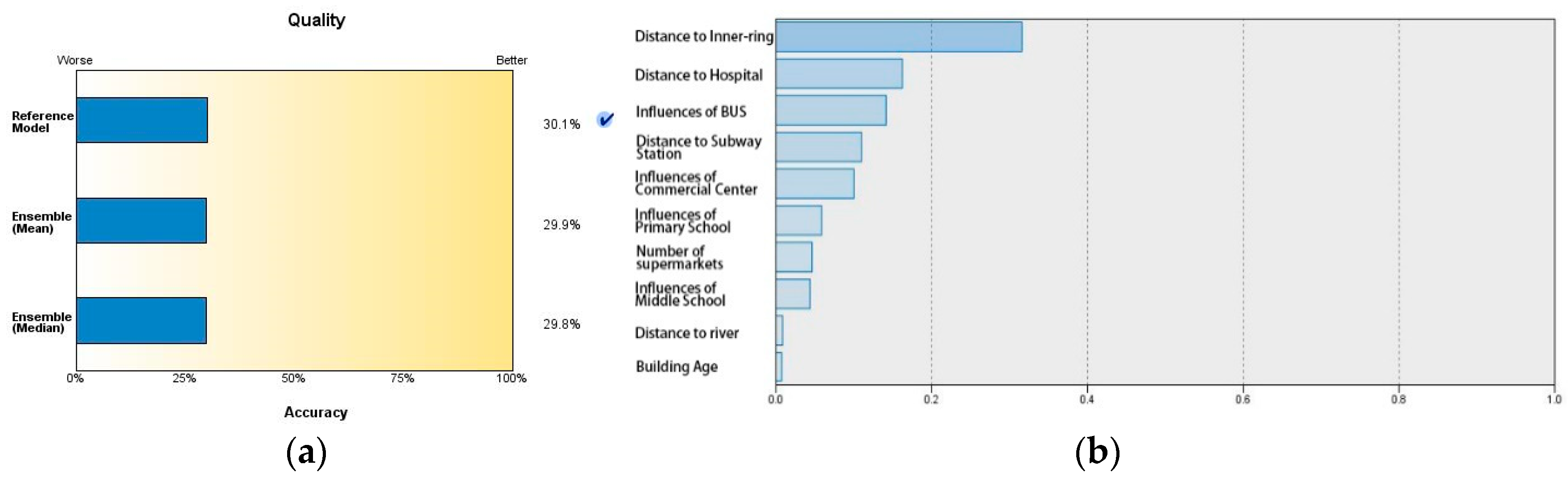
The above table shows only the strength of correlation between housing price and each factor, but not the collinear relation between these factors. Therefore, another round of calculation using the SPSS automatic linear regression equation is conducted, setting house price as the dependent variable, the rest of the factors as independent variables, and using forward stepwise regression as the regression method. The results are presented in Figure 2.

Setting housing price as the dependent variable y and the influence factors independent variables x₁, x₂, …, x_n, the Hedonic linear regression model is shown in Equation (1), where ${\beta }_0$ is the regression constant, ${\beta }_1$ to ${\beta }_n$ are respectively the regression coefficient of each factor, and $\epsilon$ the random error.

$$y={\beta }_0+{\beta }_1{x}_1+{\beta }_2{x}_2+\cdots +{\beta }_n{x}_n+\epsilon$$

(1)

In the regular hedonic regression model, as the multi-collinearity factor is taken into consideration, the strength of correlation between housing price and each influence factor in the model changes. The correlation is still strongest between housing price and the distance to the inner ring, but the factor of the commercial center, which had the second strongest correlation, drops to fifth place. Hospitals, buses and subways rank at the second, third and fourth place respectively. The highest overall fit of linear regression equation calculated is 30.1%. Three factors, water area, population density and green space are of the weakest correlation with housing price. Out of the three, the water area factor shows insignificant correlation.

3.3. Geographic Weighted Regression Analysis Based on ArcGIS

In the previous regression analysis lies a presumption that the relations between variables are homogenous, where the local characteristics between them are concealed, that is, all the factors in the study area are presumed to have the same influence coefficient. This presumption ignores the spatial relationship between the various factors, and on this basis, the same factors are used for the geographical weighted regression analysis. The GWR module incorporated in the ArcGIS platform uses independent formulas for each element in the dataset and combines the dependent and explanatory variables for elements that fall within the bandwidth of each target element.

In comparison with Equation (1), according to the first law of geography, the regression coefficients ${\beta }_1$ to ${\beta }_n$, the regression constant, random error and so on all change with the spatial position of different sample points in the GWR model (Equation (2)). In the formula, $\left(u_i,v_i\right)$ represents the coordinate of sampling point $i$; ${\beta }_k\left(u_i,v_i\right)$ is the number $k$ regression parameter of sampling point $i$, and is a function of the geographical position; $p$ is the number of explanatory variables; and ${\epsilon }_i$ the random error of sampling point $i$.

$$y_i={\beta }_0\left(u_i,v_i\right)+{{\displaystyle \sum }}_{k=1}^p{\beta }_k\left(u_i,v_i\right)x_{ik}+{\epsilon }_{i}i=1,2,3,\dots ,n$$

(2)

In ArcGIS’s own GWR analysis module [37], selecting the surface element layer of spatial units as input element, the average price as the dependent variable, the remaining 13 elements of the influence factors as explanatory variables, and import these into the model then calculating gives results that are shown in

Table 3. Output 1 of the geographically weighted regression (GWR) model analysis.

Objectid	Varname	Variable	Definition
1	Bandwidth	9229.90595
2	ResidualSquares	32,298,485,006.205433
3	EffectiveNumber	42.368431
4	Sigma	4605.678949
5	AICc	30,870.476555
6	R2	0.359273
7	R2Adjusted	0.341865
8	Dependent Field	0	Average price
9	Explanatory Field	1	Population density
10	Explanatory Field	2	Building Age
11	Explanatory Field	3	Distance to river
12	Explanatory Field	4	Distance to inner-ring
13	Explanatory Field	5	Number of supermarkets
14	Explanatory Field	6	Hierarchy of commercial center
15	Explanatory Field	7	Hierarchy of bus system
16	Explanatory Field	8	Hierarchy of primary school
17	Explanatory Field	9	Hierarchy of middle school
18	Explanatory Field	10	Hierarchy of green space
19	Explanatory Field	11	Distance to hospital
20	Explanatory Field	12	Distance to Subway station

and Figure 5. Multiple rounds of calculation were performed in the present study to examine the influence of different combinations of factors on the fitting degree. Finally, excluding the factor of water area which has an insignificant correlation, the fitting degree (R²) reaches 0.3419 at its highest.

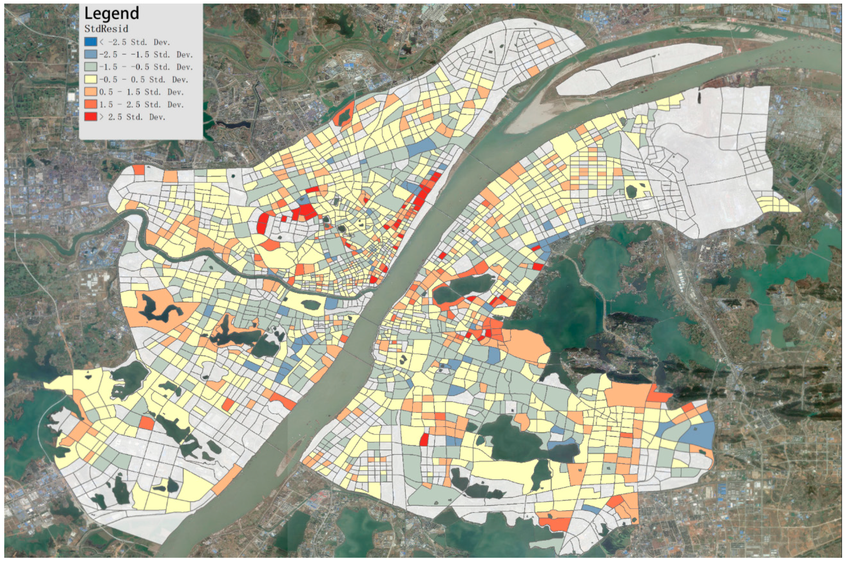
In the GWR model, standard residual 0 means the predicted value calculated by the model is completely consistent with the observed value (that is, the original input value). The further that a deviation is from 0 indicates that the model offers a weaker explanation of reasons behind the housing price. The spatial units in the yellow color which represents a deviation between −0.5 to +0.5 can be considered areas with a good explanation. However, areas marked with an absolute value of deviation over 2.5 can be regarded as seriously deviated from the model and need targeted examination and explanation. In addition, certain spatial units in the selected inner city area are not completely covered due to the problems of null values or missing data, and are presented as white areas which are not included in the calculation (Figure 3).

According to the formula for calculating standard residuals, a positive value means that the predicted value is lower than the observed value, i.e., the actual housing price is higher than the predicted value, and a negative value is the opposite. Therefore, the dark red area in the diagram, with a value above 2.5, marks a housing price much higher than the predicted value, while the dark blue area of −2.5, a much lower price than predicted. In the present study, the spatial units with standard residuals greater than 2.5 are all positive, so the main reasons behind this are analyzed.

The spatial units with standard residuals greater than 2.5 are mainly distributed in three areas, i.e., both sides of the Second Bridge of the Yangtze River, Wangjiadun Central Business District, Hongshan Square and the surrounding area of Shahu Lake, plus several spatial units sporadically distributed around the East Lake and the South Lake. The residential properties in these spatial units are then specifically analyzed: in the South Lake area, the above 2.5 property is the Golden Saint-Emilion residential area. Though not a villa property, its price is much higher than the average in the area; considering the Wangjidun area is planned as the Central Business District of the city and at present, its public facilities have not yet been completed, it high housing price is not solely backed by the surrounding spatial elements; the spatial units around the Second Bridge of the Yangtze River and those around the East Lake area share many similarities, in that, the housing prices of these areas far exceed those of their surrounding areas. Most residential properties in these areas, except the older ones, have prices close to or over 40,000 Yuan/m², and certain properties such as Wuhan Xintiandi (New World), Yujiang Jingcheng and Tiandi Yuting have prices as high as 70,000 Yuan/m². The reasons behind these high prices could be the enormous influence of the river view (water features).

3.4. Regression Analysis Based on Artificial Neural Network (ANN)

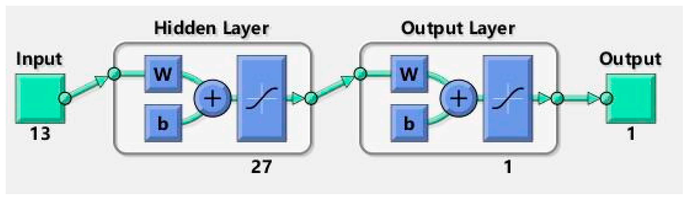
The two regression models used in the previous analysis are still essentially linear models, but the influence of spatial factors on housing price is often non-linear. Therefore, many studies process the initial values of the factors in non-linear functions before putting them into the regression model. For non-linear regression prediction, one of the more widely used methods is the artificial neural network (ANN). In the present study, the ANN toolbox in Matlab is used to perform the calculations where the 13 influence factors in the GWR model were used as independent variables and housing prices as the dependent variable. After various tests and adjustments, the final selected network type is feed-forward backprop, using the Bayesian regulation as the training function (trainbr), and the mean squared error (MSE) as the performance function, with one hidden layer and 27 hidden nodes (See Figure 4).

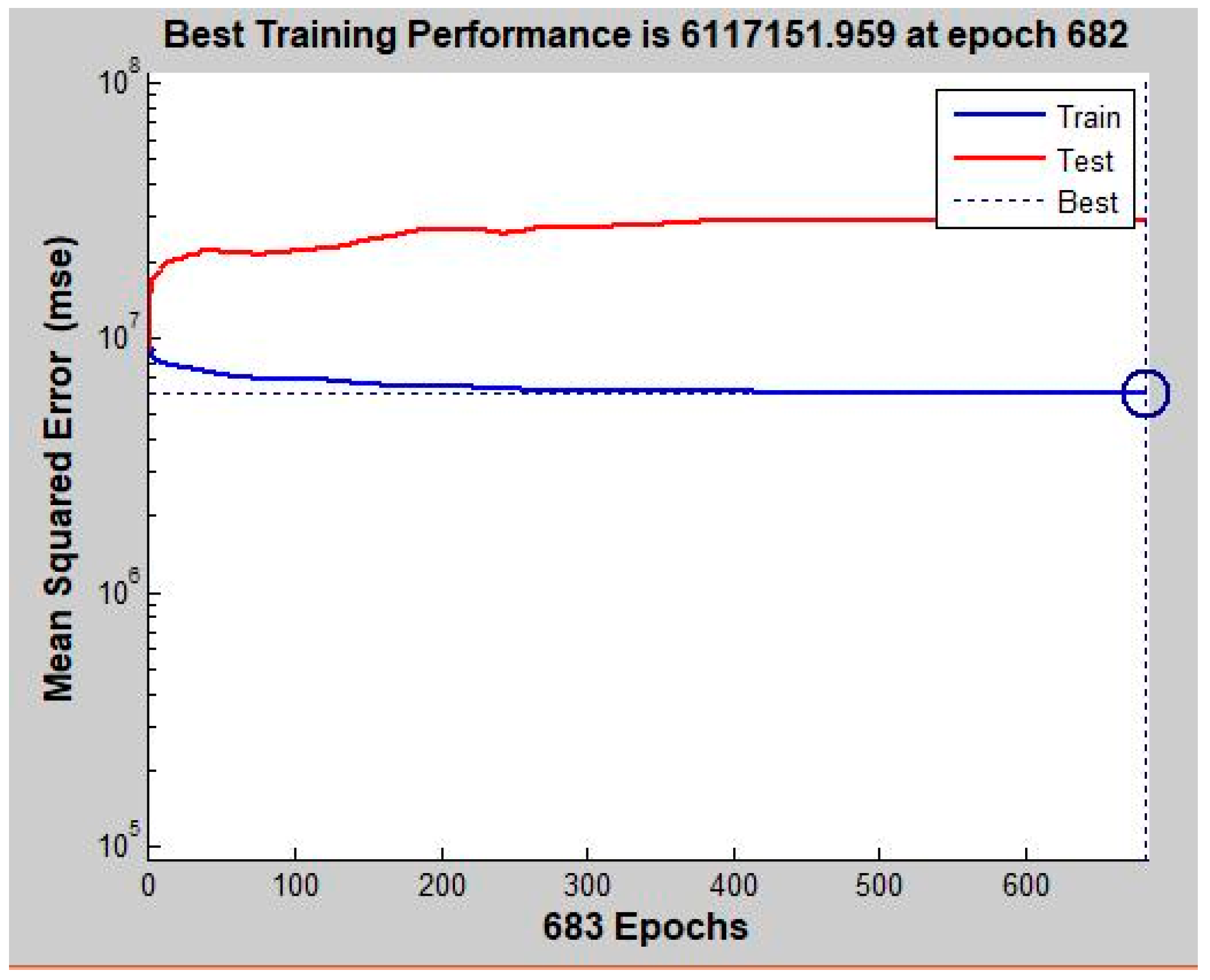
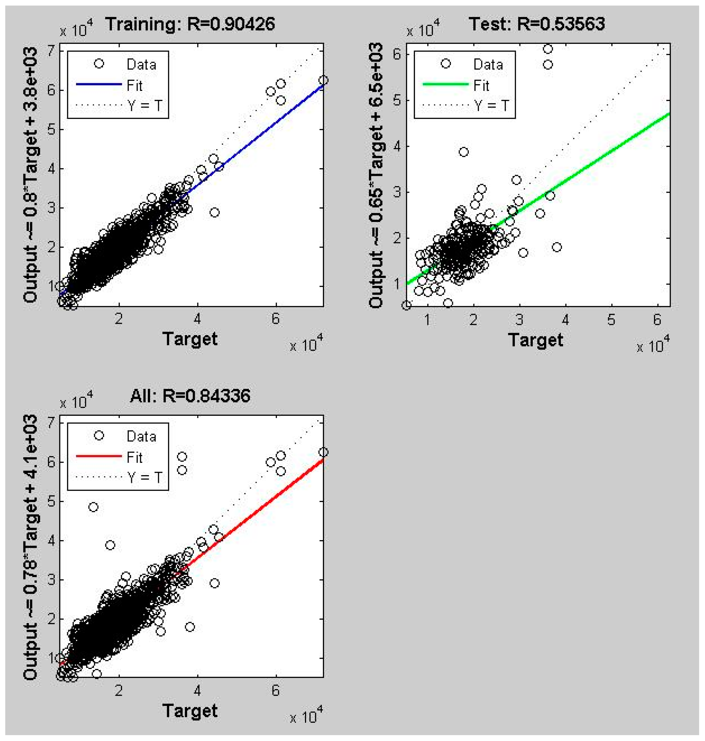
Then the matrix of the 1565 groups of variables are used as the input value X, while value Y stands for the housing price corresponding to each group of variables. All values are imported into the ANN for learning and calculation where all variables are divided into three groups, namely Training (the training variables), Test (the test variables), and Target (the target variables). The calculation process is shown in Figure 5. It can be seen that the best training performance is found at epoch 683 of the training. The final regression fitting result is shown in Figure 6. Based on the calculation, the R coefficient between the predicted housing price and the original value is 0.843360, and the R-square is 0.7112.

Compared with the GWR model, the artificial neural network can be regarded as an independent variable processing function in a trained housing price model. Imported into the model, the original values of the 13 impact factors are processed by a specific procedure, which generates the corresponding predicted housing price. This processing procedure can be viewed as ${\beta }_n$ in Equation (1) but, like the hedonic linear model, the processing procedure does not consider changes in coefficient of the spatial influence factors. Therefore, housing price values generated by the ANN prediction are imported back into the GWR model and the results of the calculation are shown in

Table 4. Output 1 of the GWR model analysis.

Objectid	Varname	Variable	Definition
1	Bandwidth	3864.70251256000
2	ResidualSquares	13,858,292,289.200000
3	EffectiveNumber	33.71935716350
4	Sigma	3008.34376754000
5	AICc	29,526.72448670000
6	R2	0.72508343686
7	R2Adjusted	0.71920920782
8	Dependent Field	0	Average price
9	Explanatory Field	1	ANN predicted value

. The R-square corresponding to the value calculated directly by the ANN is 0.7251, which is better than the original 0.7112. It can be seen that the best fit can be obtained by integrating the non-linear prediction of the ANN and the varying spatial coefficients of the influence factors of the GWR model, and this result also proves that the factors selected in the present study can explain most of the reasons that determine housing prices.

4. Discussion

The kernel density method is used in the calculation for part of the influence factors and, thus, the result is also compared with that of the conventional geometric distance method. Similarly, the distance parameters can be imported into the explanatory factors in the GWR model calculation and the result is presented in

Table 5. Output 2 of the GWR model analysis.

Objectid	Varname	Variable	Definition
1	Bandwidth	15,816.098690
2	ResidualSquares	33,477,816,748.300000
3	EffectiveNumber	29.370509
4	Sigma	4669.123292
5	AICc	30,910.992512
6	R2	0.335877
7	R2Adjusted	0.3236077
8	Dependent Field	0	Average price
9	Explanatory Field	1	Population density
10	Explanatory Field	2	Age
11	Explanatory Field	3	Distance to river
12	Explanatory Field	4	Distance to inner ring
13	Explanatory Field	5	Distance to hospital
14	Explanatory Field	6	Subway
15	Explanatory Field	7	Number of supermarkets
16	Explanatory Field	8	Distance to commercial center
17	Explanatory Field	9	Distance to middle school
18	Explanatory Field	10	Distance to primary school
19	Explanatory Field	11	Distance to green space
20	Explanatory Field	12	Density of bus routes and network

. A comparison with Table 3 shows that using the kernel density method to grade some of the factor values produces a better fit and a lower AICc. (A measurement used to compare the performances of different regression models). Therefore, the model behind Table 2, with lower AICc values, is considered a more optimal model. This also proves that the kernel density method can be used to optimize the explanatory variables imported into the GWR model and offer a better understanding of the actual usage of urban public facilities.

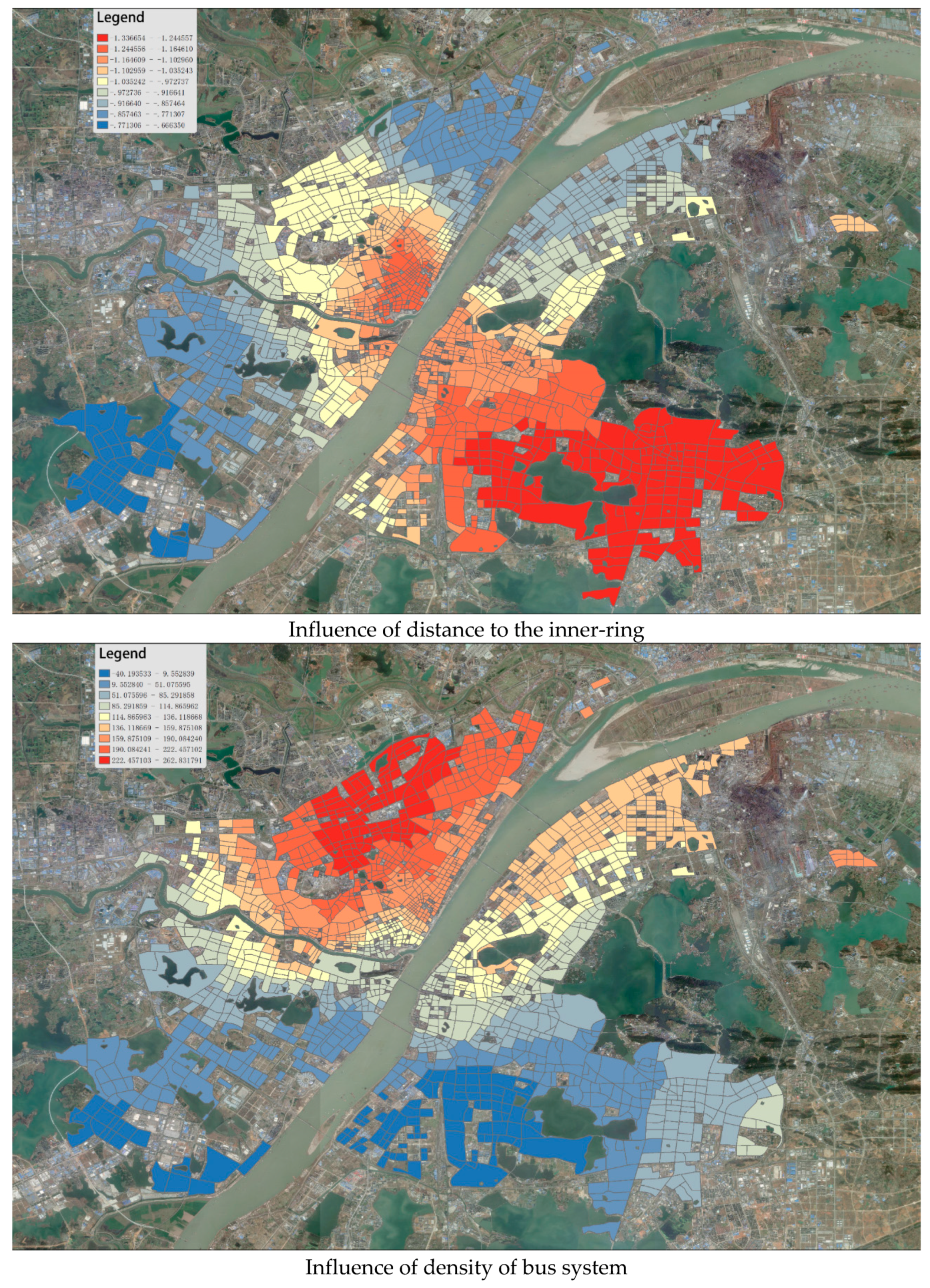
Comparing the results of the regular hedonic linear regression model and GWR model, the latter, with adjustable weights of local spatial influence, offers a higher degree of fitting, while the factors with insignificant correlation with housing price can be removed from the GWR model to improve the modelling result. For each sampling point in the GWR model, varying coefficients of influence factors are generated by the model, and can then be further analyzed through the features of spatial changes caused by these influencing coefficients so as to evaluate the intensity of influence by various factors and at different spatial locations. The spatial variation of the coefficients of some influence factors generated by the GWR model is shown in Figure 7.

(1) The influence coefficient of the factor, distance to inner ring, on housing price is negative, i.e., the further away from the inner ring of the city, the lower the housing price (due to the negative conversion, inside of the inner ring area, the further away the distance is, the higher the housing price). The absolute value of the influence coefficient is the highest in the Optics Valley area, and gradually decreases towards the outside, achieving a balance when gradually approaching the inner ring.

(2) The influence factor, hierarchy of the bus transit, has a positive correlation to housing price, i.e., the higher the hierarchy of the bus transit is, the higher the housing price. However, in the study area as a whole, the coefficient of influence decreases gradually from north to south, and even negative correlation occurs in some areas. This can also be interpreted as meaning that, in the southern part of the study area, including the Nanhu area in Hongshan District, the Baishazhou area, and the Houguanhu area in Caidian District, the density of bus routes and network is much lower than that in other areas.

When either the hedonic or the GWR model is used alone, the degree of fit in the causal analysis of housing prices remains low. One possible reason is the difference in sample size. As the relationship between housing price and influence factors is not a simple linear relationship, the validity of the regression model decreases with larger sample size. Therefore, the introduction of the artificial neural network, a non-linear regression model, combined with the GWR model, substantially improves the degree of fit. Another reason may be that certain major influence factors are not considered when selecting the explanatory factors for the study, such as urban land-use planning. Comparing the three regression models, it can be seen that the regular hedonic linear model can be used together with SPSS to compare the importance of various influence factors, and thus can improve the fitting degree by eliminating the unrelated factors through correlation analysis; while the GWR model offers a better explanation than the hedonic model and its advantage lies in its interpretation of the causes of housing prices by measuring the spatial variation in the influence of each factor. The GWR model not only recognizes the abnormality in housing prices within a city and whether it is a deviation from its actual price, it can also allocate the analysis of various influence factors into specific spatial units and, therefore, provides references for subsequent decision-making in urban planning; the artificial neural network model breaks through certain limitations of the linear regression of the aforementioned two models. Its advantage is that the degree of fitting can be substantially improved. However, due to the fact that its calculation process is like a black box in that it offers no explanation nor a regression formula, the ANN model can only be used to predict housing price but not to analyze the importance of each factor or to perform a spatial analysis of its influence.

5. Conclusions

As data acquisition is considered one of the biggest difficulties in the study of housing prices [38], the present study uses an approach using multiple data sources in related models and thus contributes to the methodology of research on housing prices. These multiple data sources, including open network data, offer opportunities to acquire more diverse types and a much greater number of sample data than previous research, and with greater timeliness, thus providing more valuable findings for the quantitative spatial analysis of cities.

From the planning perspective, the present study chooses various factors that may influence housing price, so as to make clear the relationship between the influence factors and housing prices as well as their variations in space. In the case study city of Wuhan, when eliminating the collinearity relationship, four influence factors show the greatest influence on housing price, namely, distance to the inner ring, distance to hospital, bus density, and distance to subway station. Due to the multi-center urban structure of Wuhan where the main urban districts are divided by the rivers, and the uneven development of these districts, variation in the influence of factors over space and the uneven distribution of public facilities and transport infrastructure can be observed. In addition, even if urban planning schemes have not yet been fully implemented, there is a positive long-term prospect of an increase of housing prices, exemplified by Wangjiadun Central Business District. In the case of Wuhan, urban elements directly controlled by city planning, including the layout of public facilities, planning and spatial location of transport etc., all have a great influence on housing price.

In the numerical calculation of the public facility factor, analysis based on the superposition of the service radius of multiple facilities offers a better explanation for housing price than the sole consideration of the shortest distance. The final combination of the ANN and GWR model adopted in the present studies helps achieve a good model fit. This result means that the selected influence factors can explain most of the factors determining housing prices, and the ANN, with the support of the other two models, can be used to analyze the importance of an individual factor and the variation of its spatial influence coefficient. In general, the contribution the present study lies in the research methodology of a combined use of multiple data sources in multiple models, which facilitates more comprehensive analysis of the reasons behind housing prices.

References

- Hu, S.; Yang, S.; Li, W.; Zhang, C.; Xu, F. Spatially non-stationary relationships between urban residential land price and impact factors in Wuhan city, China. Appl. Geogr. 2016, 68, 48–56. [Google Scholar] [CrossRef]
- Straszheim, M.R. An Econometric Analysis of the Urban Housing Market; Nber Books; Columbia University Press: New York, NY, USA, 1975. [Google Scholar]
- Rosen, S. Hedonic Prices and Implicit Markets: Product Differentiation in Pure Competition. J. Polit. Econ. 1974, 82, 34–55. [Google Scholar] [CrossRef]
- Butler, R.V. The Specification of Hedonic Indexes for Urban Housing. Land Econ. 1982, 58, 96–108. [Google Scholar] [CrossRef]
- Adair, A.; McGreal, S.; Smyth, A.; Cooper, J.; Ryley, T. House Prices and Accessibility: The Testing of Relationships within the Belfast Urban Area. Hous. Stud. 2000, 15, 699–716. [Google Scholar] [CrossRef]
- Basu, S.; Thibodeau, T.G. Analysis of Spatial Autocorrelation in House Prices. J. Real Estate Finan. Econ. 1998, 17, 61–85. [Google Scholar] [CrossRef]
- Jim, C.Y.; Chen, W.Y. Impacts of urban environmental elements on residential housing prices in Guangzhou (China). Landsc. Urban Plan. 2006, 78, 422–434. [Google Scholar] [CrossRef]
- Law, S. Defining Street-based Local Area and measuring its effect on house price using a hedonic price approach: The case study of Metropolitan London. Cities 2017, 60, 166–179. [Google Scholar] [CrossRef]
- Sunak, Y.; Madlener, R. The impact of wind farms on property values: A locally weighted hedonic pricing model. Pap. Reg. Sci. 2017, 96, 423–444. [Google Scholar] [CrossRef]
- Atkinson, S.E.; Crocker, T.D. A Bayesian Approach to Assessing the Robustness of Hedonic Property Value Studies. J. Appl. Econ. 1987, 2, 27–45. [Google Scholar] [CrossRef]
- Smith, V.K.; Huang, J.C. Can Markets Value Air Quality? A Meta-Analysis of Hedonic Property Value Models. J. Polit. Econ. 1995, 103, 209–227. [Google Scholar] [CrossRef]
- Kuminoff, N.V.; Parmeter, C.F.; Pope, J.C. Which hedonic models can we trust to recover the marginal willingness to pay for environmental amenities? J. Environ. Econ. Manag. 2010, 60, 145–160. [Google Scholar] [CrossRef]
- Rasmussen, D.W.; Zuehlke, T.W. On the choice of functional form for hedonic price functions. Appl. Econ. 1988, 22, 431–438. [Google Scholar] [CrossRef]
- Halvorsen, R.; Pollakowski, H.O. Choice of Functional Form of Hedonic Price Equations. J. Urban Econ. 1981, 10, 37–49. [Google Scholar] [CrossRef]
- Cassel, E.; Mendelsohn, R. The choice of functional forms for hedonic price equations: Comment. J. Urban Econ. 1985, 18, 135–142. [Google Scholar] [CrossRef]
- Do, A.Q.; Grudnitski, G. A Neural Network Analysis of the Effect of Age on Housing Values. J. Real Estate Res. 1993, 8, 253–264. [Google Scholar]
- Selim, H. Determinants of house prices in Turkey: Hedonic regression versus artificial neural network. Expert Syst. Appl. 2009, 36, 2843–2852. [Google Scholar] [CrossRef]
- Tobler, W.R. A Computer Movie Simulating Urban Growth in the Detroit Region. Econ. Geogr. 1970, 46 (Suppl. 1), 234–240. [Google Scholar] [CrossRef]
- Brunsdon, C.; Fotheringham, A.S.; Charlton, M. Some Notes on Parametric Significance Tests for Geographically Weighted Regression. J. Reg. Sci. 1999, 39, 497–524. [Google Scholar] [CrossRef]
- Brunsdon, C.; Fotheringham, A.S.; Charlton, M.E. Geographically Weighted Regression: A Method for Exploring Spatial Nonstationarity. Geogr. Anal. 1996, 28, 281–298. [Google Scholar] [CrossRef]
- Nakaya, T. Local spatial interaction modelling based on the geographically weighted regression approach. Geojournal 2001, 53, 347–358. [Google Scholar] [CrossRef]
- Yrigoyen, C.C.; Rodríguez, I.G.; Otero, J.V. Modeling spatial variations in household disposable income with Geographically Weighted Regression. MPRA Pap. 2007, 50, 321–360. [Google Scholar]
- You, W.; Zang, Z.; Zhang, L.; Li, Z.; Chen, D.; Zhang, G. Estimating ground-level PM10 concentration in northwestern China using geographically weighted regression based on satellite AOD combined with CALIPSO and MODIS fire count. Remote Sens. Environ. 2015, 168, 276–285. [Google Scholar] [CrossRef]
- Ge, Y.; Song, Y.; Wang, J.; Liu, W.; Ren, Z.; Peng, J.; Lu, B. Geographically weighted regression-based determinants of malaria incidences in northern China. Trans. GIS 2016, 21. [Google Scholar] [CrossRef]
- Bitter, C.; Mulligan, G.F.; Dall’Erba, S. Incorporating spatial variation in housing attribute prices: A comparison of geographically weighted regression and the spatial expansion method. J. Geogr. Syst. 2007, 9, 7–27. [Google Scholar] [CrossRef] [Green Version]
- Lu, B.; Charlton, M.; Harris, P.; Fotheringham, A.S. Geographically weighted regression with a non-Euclidean distance metric: A case study using hedonic house price data. Int. J. Geogr. Inf. Sci. 2014, 28, 660–681. [Google Scholar] [CrossRef]
- Efthymiou, D.; Antoniou, C. How do transport infrastructure and policies affect house prices and rents? Evidence from Athens, Greece. Transp. Res. Part A Policy Pract. 2013, 52, 1–22. [Google Scholar] [CrossRef]
- Mulley, C. Accessibility and residential land value uplift: Identifying spatial variations in the accessibility impacts of a bus transitway. Urban Stud. 2014, 51, 1707–1724. [Google Scholar] [CrossRef]
- Dziauddin, M.F.; Powe, N.; Alvanides, S. Estimating the Effects of Light Rail Transit (LRT) System on Residential Property Values Using Geographically Weighted Regression (GWR). Appl. Spat. Anal. Policy 2015, 8, 1–25. [Google Scholar] [CrossRef]
- Huang, B.; Wu, B.; Barry, M. Geographically and temporally weighted regression for modeling spatio-temporal variation in house prices. Int. J. Geogr. Inf. Sci. 2010, 24, 383–401. [Google Scholar] [CrossRef]
- Wu, B.; Li, R.; Huang, B. A geographically and temporally weighted autoregressive model with application to housing prices. Int. J. Geogr. Inf. Sci. 2014, 28, 1186–1204. [Google Scholar] [CrossRef]
- Fotheringham, A.S.; Crespo, R.; Yao, J. Exploring, modelling and predicting spatiotemporal variations in house prices. Ann. Reg. Sci. 2015, 54, 417–436. [Google Scholar] [CrossRef]
- Wu, C.; Ye, X.; Ren, F.; Wan, Y.; Ning, P.; Du, Q. Spatial and Social Media Data Analytics of Housing Prices in Shenzhen, China. PLoS ONE 2016, 11, e0164553. [Google Scholar] [CrossRef] [PubMed]
- Cai, J.; Huang, B.; Song, Y. Using multi-source geospatial big data to identify the structure of polycentric cities. Remote Sens. Environ. 2017, 202, 210–221. [Google Scholar] [CrossRef]
- Glaeser, E.L.; Kominers, S.D.; Luca, M.; Naik, N. Big data and big cities: The promises and limitations of improved measures of urban life. Econ. Inquir. 2018, 56, 114–137. [Google Scholar] [CrossRef]
- Wang, D.; Huang, W. Hedonic House Pricing Method and Its Application in Urban Studies. City Plan. Rev. 2005, 29, 62–71. [Google Scholar]
- Esri. Geographically Weighted Regression (GWR) (Spatial Statistics). 2013. Available online: http://resources.arcgis.com/en/help/main/10.1/index.html#//005p00000021000000 (accessed on 8 March 2018).
- Wang, D.; Huang, W. Effect of Urban Environment on Residential Property Values by Hedonic Method: A Case Study of Shanghai. City Plan. Rev. 2007, 31, 34–41. [Google Scholar]
Figure 1.
Hierarchical influences of commercial centers and the spatial distribution of housing properties.
Figure 2.
Regression model analysis results of factors. (a) Model regression accuracy; (b) strength of correlation with each factor.
Figure 3.
Spatial distribution of standard residuals based on the GWR model.
Figure 4.
Diagram of the artificial neural network (ANN) structure.
Figure 5.
Mean variance curve.
Figure 6.
Regression fitting curve.
Figure 7.
The spatial coefficients of some influencing factors.