Soil Organic Carbon Baselines for Land Degradation Neutrality: Map Accuracy and Cost Tradeoffs with Respect to Complexity in Otjozondjupa, Namibia

Abstract

Recent estimates show that one third of the world’s land and water resources are highly or moderately degraded. Global economic losses from land degradation (LD) are as high as USD $10.6 trillion annually. These trends catalyzed a call for avoiding future LD, reducing ongoing LD, and reversing past LD, which has culminated in the adoption of Sustainable Development Goal (SDG) Target 15.3 which aims to achieve global land degradation neutrality (LDN) by 2030. The political momentum and increased body of scientific literature have led to calls for a ‘new science of LDN’ and highlighted the practical challenges of implementing LDN. The aim of the present study was to derive LDN soil organic carbon (SOC) stock baseline maps by comparing different digital soil mapping (DSM) methods and sampling densities in a case study (Otjozondjupa, Namibia) and evaluate each approach with respect to complexity, cost, and map accuracy. The mean absolute error (MAE) leveled off after 100 samples were included in the DSM models resulting in a cost tradeoff for additional soil sample collection. If capacity is sufficient, the random forest DSM method out-performed other methods, but the improvement from using this more complex method compared to interpolating the soil sample data by ordinary kriging was minimal. The lessons learned while developing the Otjozondjupa LDN SOC baseline provide valuable insights for others who are responsible for developing LDN baselines elsewhere.

1. Introduction

The state of the world’s land resources is increasingly disturbing. In 2011, the FAO [1] estimated that 33% of the world’s land and water resources are highly or moderately degraded (land degradation is defined as a loss of ecosystem functionality that affects the biological or economic productivity due to unsustainable human activity in combination with natural processes [2]. Arable land, in particular, shows alarming trends [3]. Recent estimates show that 52% of agricultural land worldwide is degraded [4]. Given that the majority of terrestrial carbon is stored in soils [5], the potential loss of carbon that is currently sequestered in soils poses an additional climate change threat beyond the loss of soil health. Global economic losses from LD start are estimated to be USD $10.6 trillion annually [4]. In Sub-Saharan Africa, alone, 180 million people are affected by LD [6].

The staggering evidence of the magnitude and rate of LD, and its continued negative impacts on food and fiber production and human well-being, catalyzed a call for avoiding future LD, reducing ongoing LD, and reversing past LD. The concept of ‘zero net land degradation’ (ZNLD) was first mentioned at the UN Convention to Combat Desertification (UNCCD) in 2011 [7]. The following year, ZNLD was proposed at the UN Conference on Sustainable Development (Rio+20). Two important events in 2015 further solidified the importance of Land Degradation Neutrality (LDN). The Sustainable Development Goals (SDGs) were adopted by the UN General Assembly and SDG Target 15.3 specifically aims to “combat desertification, restore degraded land and soil, including land affected by desertification, drought and floods, and strive to achieve a land degradation-neutral world” by 2030. Later that year, during the twelfth UNCCD Conference of the Parties (COP), parties decided to integrate LDN into the implementation of the UNCCD.

The political momentum (i) translated into new debates, and (ii) increased the body of scientific literature including calls for a ‘new science of LDN’ [8]. The LDN debates, thus far, have focused on its feasibility [9,10], its scientific conceptual framework [11,12], practical issues concerning operationalization [8,13], and its potential to unify the three Rio Conventions [14]. Meanwhile, the scientific community agreed to connect LDN to the SDG Target 15.3 indicator, which is the ‘proportion of land that is degraded over total land area,’ and this is measured with three sub-indicators: (i) land cover; (ii) land productivity; and (iii) carbon stocks above and below ground [15]. By linking LDN to SDG15.3, earlier UNCCD indicators on nutrition, water, and food security are now removed [9]. Lastly, the Science and Policy Interface (SPI) of the UNCCD was tasked with providing technical support to national governments that were encouraged to set voluntary targets [15], including 14 pilot countries tasked with developing baselines of the three indicators. Separately, a review of available LDN methodologies was completed for two of the pilot countries emphasizing how the concept can be applied in contrasting regions, from flat desserts to hilly rainforests [16,17].

The aim of the present study was to derive LDN SOC stock baseline maps by comparing different methods and sampling densities for derivation of SOC baselines in a case study (Otjozondjupa, Namibia) and evaluate each approach with respect to complexity, cost, and map accuracy. Even though the results are site-specific, the Otjozondjupa example will illustrate cost-benefit trade-offs of different digital soil mapping methods and sampling densities and, thus, provide new insights and guidance for future LDN SOC stock baseline mapping in other areas. We expect that the lessons learned are particularly useful for government departments that are responsible for developing LDN baselines elsewhere.

2. Methods

2.1. Area of Interest

The sparsely populated Otjozondjupa Region with 1.4 inhabitant km⁻² [18] is situated in Northeast Namibia (Figure 1), and it is one of seven LD hotspots in the country [19]. Otjozondjupa covers about 105,000 km² and is characterized by grassland and sparsely-vegetated shrubland with small areas of closed canopy forest (Figure 1). The land tenure is predominantly private ownership except for community lands in northeast districts. Land use is mostly rangeland cattle farming, much of it being extensive commercial cattle farming, grain production, and a large proportion of smallholder subsistence agriculture, mainly in the communal lands [20]. Namibia is the most arid country in sub-Saharan Africa and prolonged droughts are well-known occurrences. These occurrences, as well as climate variability, are likely to increase in the future [21].

2.2. Study Scope and Design

In the present study we followed the tiered approach recommended by the UNCCD’s LDN Target Setting Programme as outlined in the methodological note on setting national LDN targets [22]. This approach calls for three levels of computation for developing a baseline map of SOC stock (in kg m⁻²) for the 0–30 cm soil layer: Tier 1, using globally-available soil maps; Tier 2, using national legacy soil maps; and Tier 3 using maps developed from newly-acquired field data. The methodological note further recommends that existing maps can be enhanced and complemented with additional field data, where possible. For the purposes of this paper, we call this enhancement approach Tier 4 in order to distinguish it from the Tier 3 approach, which does not use the existing spatial data as an input. In Namibia there was no national SOC baseline available, and Tier 2 was, therefore, excluded.

In the absence of local data, the recommended default global SOC dataset is SoilGrids250m (www.soilgrids.org) [23], which is made available by ISRIC–World Soil Information [22]. SoilGrids250m is a series of freely-available global gridded maps of basic soil properties and classes at 250 m resolution. SoilGrids250m maps were developed by combining field data from about 150,000 soil sampling sites and 158 remotely-sensed covariates with global coverage in a machine-learning model [23]. Here we used a SoilGrids250m-derived SOC stock map as the Tier 1 baseline map. As a Tier 3 approach we developed a SOC baseline map using ordinary kriging (OK) from newly-acquired soil sample data, and we developed two Tier 4 baseline maps from soil sample data and the SoilGrids250m product using different digital soil mapping methods with different levels of complexity (see Section 2.5), one using the SoilGrids250m SOC stock map and the other using 222 covariate layers that included the layers used to develop the SoilGrids250m maps supplemented with layers of biophysical Earth surface properties that were available at continental and regional scales. To test the effect of different sampling densities on map accuracy, in total 48 maps were produced (three mapping methods × 16 different sample sizes: 20, 30, 40, …, 170), in addition to the Tier 1 baseline map.

2.3. Soil Sampling and Soil Analyses

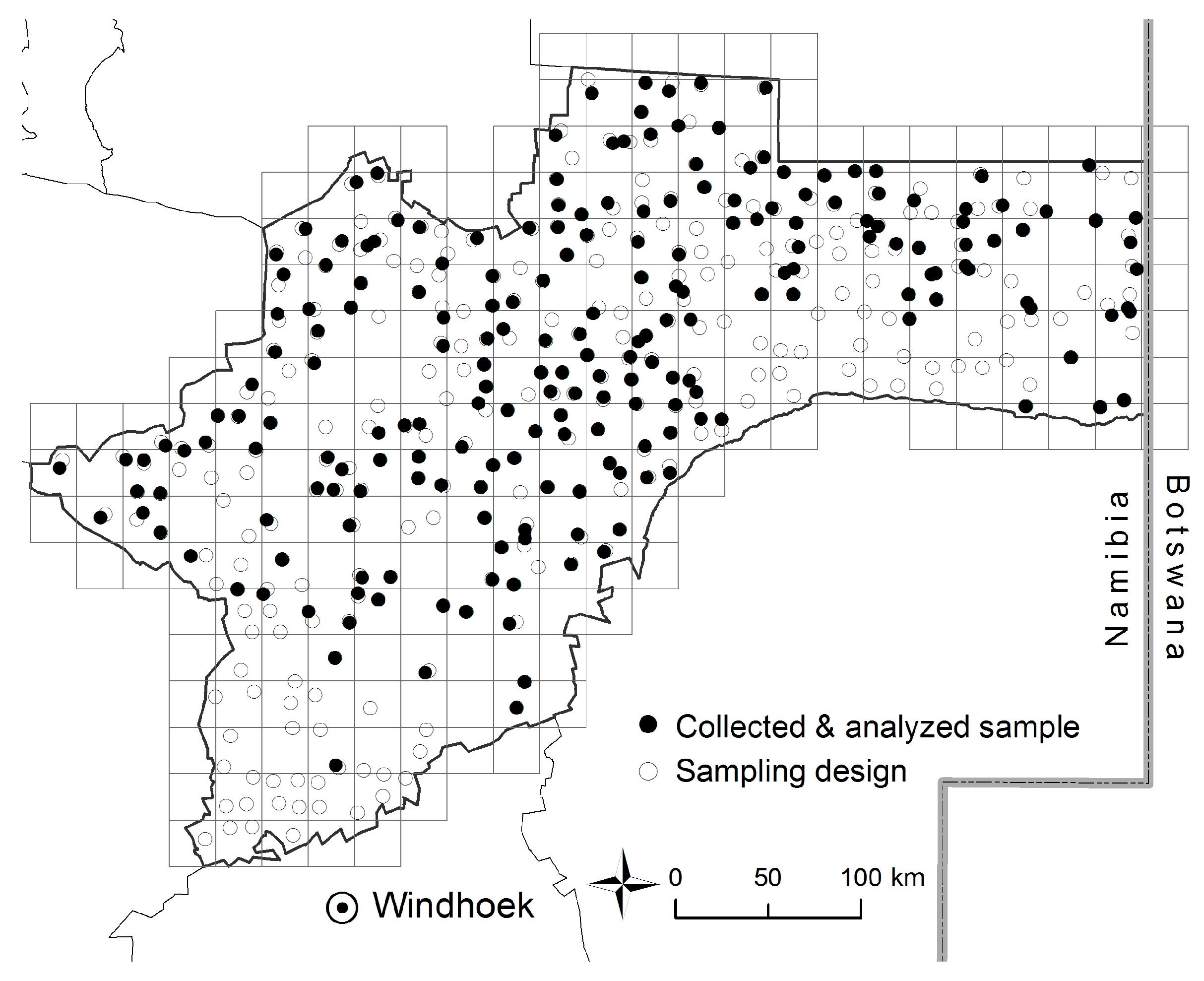
2.3.1. Sampling Design

Soil sample locations were selected across Otjozondjupa using a directed stratified sampling design. This method takes advantage of available and assumed relevant spatial reference information that directs the selection of sampling locations in such a way that areas with higher variability are more intensively sampled and areas which are relative homogenous are less intensively sampled. Sampling locations are, thus, selected successively, guided by the variation in the reference map. The basic principle behind the sampling method is that if data from the reference map at the selected sampling locations are interpolated using inverse distance squared weighting [24], the resulting map should be as similar as possible to the reference map (i.e., have the smallest MAE [25,26]. Here we used the SOC map derived from SoilGrids250m as the reference map for the selection of sampling locations. For stratification, the region was divided into 25 × 25 km grid cells. The reference map was smoothed using 3 × 3 cells mean filtering prior to selection of sampling locations. We transformed the mapped SOC stock values with a natural logarithm to obtain a normal distribution. The log-transformed SOC map was used for directing samples allocation. Further boundary conditions in the sample selection process were (i) a maximum of three samples to be located within one 25 × 25 km grid cell; (ii) the minimum distance between two samples should be at least 10 km; and (iii) points should not be assigned within a buffer of 5 km along the region border.

2.3.2. Soil Sample Collection and Laboratory Analyses

We aimed to sample 325 locations. Each location contained four sub-plots, one central plot and three peripheral subplots equally distributed along the perimeter of a 5 to 6 m radius circle (i.e., a sample support of 0.01 ha). The procedure for taking a composite sample for SOC analysis was as follows:

• Extract soil from the center of each of the four sub-plots to a depth of 30 cm using a soil auger. Record the exact auger depth at each sub-plot.
• Bulk samples from each subplot together in a bucket and mix the soil thoroughly.
• Take a representative 1 kg sub-sample from the bucket and place it in a paper bag. Place the paper bag in a clear plastic bag (double bag) and place a paper label inside the outer one with details seen from outside. Air-dry the sample.

Bulk density samples were collected from the center sub-plot. The procedure was as follows:

Dig a hole using a shovel/hoe to 20–30 cm depth, vertically cut one side using a machete to have a flat surface. Using a hammer, firmly insert the core sampler at 15 cm depth until the cone is at level with the vertical soil surface. Carefully, take out soil around the core, and place a machete on the inner side of the core and gently remove it. Smoothly cut off the sides using a knife.

Soil samples were analyzed for dry mass and SOC at the Ministry of Agriculture, Water, and Forestry using the Walkley-Black method [27,28].

2.4. Mapping Methods

The four mapping approaches (Tier 1, 3, and 4 approaches) range in degrees of complexity, from a spatial interpolation method that is now standard in most geographic information systems (GIS) software packages and can be readily applied, to more complex DSM approaches (

Table 1. A summary of the requirements for adopting different methods for deriving baseline soil organic carbon stock maps. SG = Soilgrids250m, OK = ordinary kriging, RK = regression kriging, RFK = regression forest kriging. GIS = geographical information system. (−) denote that it is not applicable to the method and (+), (++), …, (+++++) denote whether the requirement is high or low, one plus-sign meaning low requirement and five plus sign meaning high requirement.

Tier (Method)	Data Requirement	Labour Requirements	Software Requirements	Skills Requirements	Budget Requirements	Overall Complexity
1 (SG)	-Soilgrids250m	-soil sampling (−) -lab analyses (−) -data preparation (+) -data analyses (−) -interpretation (+) -reporting (+)	-GIS	-GIS	-labour (+) -software (+) *	Very low
2 (OK)	-Local soil sample data	-soil sampling (+) -lab analyses (+++) -data preparation (++) -data analyses (++) -interpretation (+) -reporting (+)	-GIS	-Sampling design -Geostatistics -GIS	-labour (++) -lab analyses (+++) -software (+) *	Low
3 (RK)	-Soilgrids250m -Local soil sample data	-soil sampling (+) -lab analyses (+++) -data preparation (+++) -data analyses (+++) -interpretation (+) -reporting (+)	-GIS -Statistical software	-Sampling design -Geostatistics -GIS	-labour (+++) -lab analyses (+++) -software (+) *	Medium
4 (RFK)	-Soilgrids250m -Local soil sample data -Covariate data	-soil sampling (+) -lab analyses (+++) -data preparation (+++++) -data analyses (+++++) -interpretation (+) -reporting (+)	-GIS -Data mining software -Statistical software	-Sampling design -Geostatistics -GIS -Data mining	-labour (+++++) -lab analyses (+++) -covariate data (++) * -software (+) *	High

Notes: *) if not open.

). The latter require more advanced programming, data preparation, and analytical skills, and are commonly used across a range of spatial scales, including at the continental and global level [23,29,30,31,32]. In order of increasing complexity, these methods are:

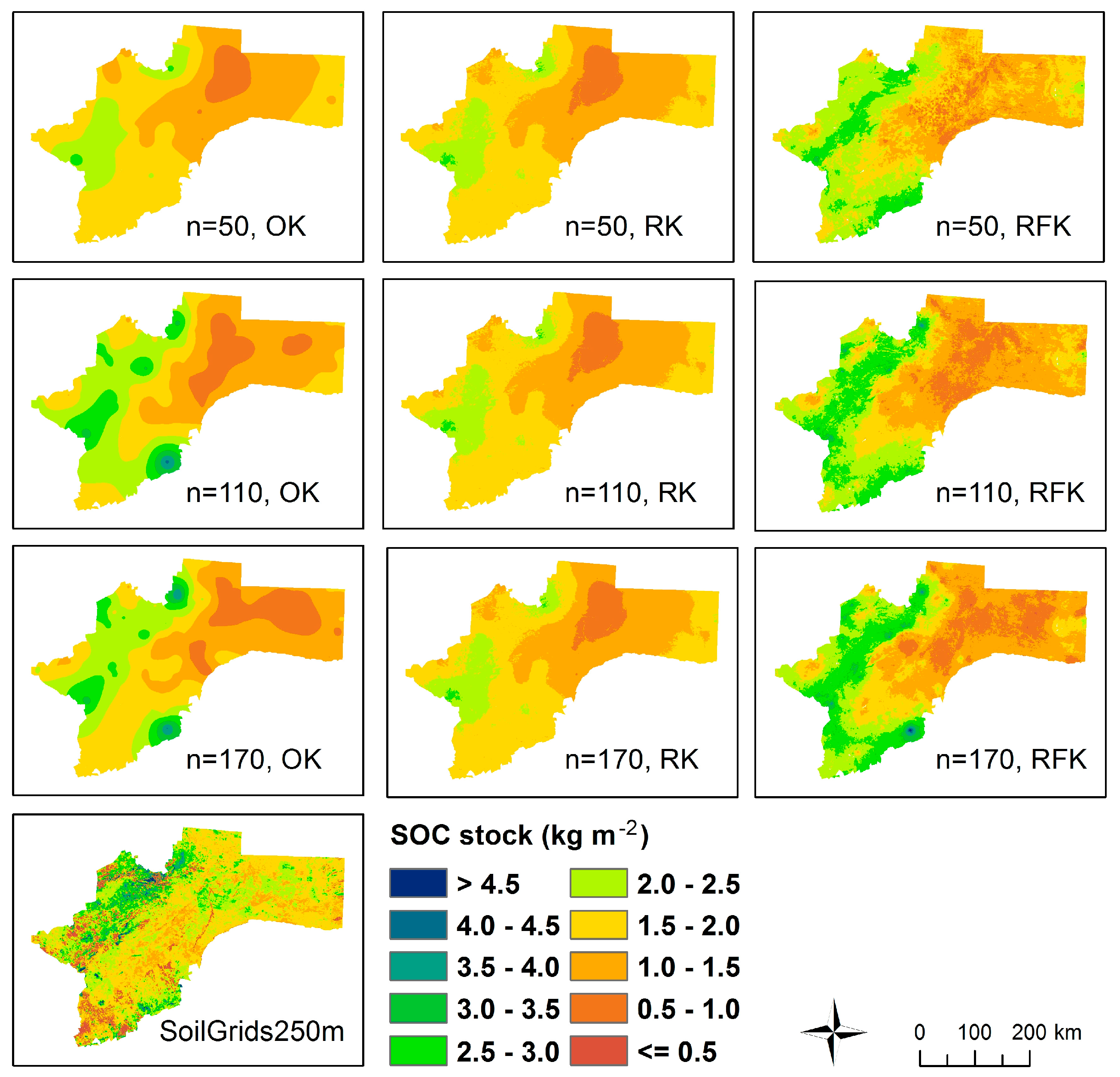
• SOC stock derived from the Soilgrids250m dataset (SG) (Tier 1);
• Ordinary kriging of the collected field data (OK) (Tier 3);
• Regression kriging of the collected field data using SG as a single covariate (RK) (Tier 4); and
• Random Forest kriging of the collected field data with a large stack (n = 222) of (freely available) environmental covariates in addition to SG (RFK) (Tier 4).

2.4.1. Soilgrids250m

The SoilGrids250m database provides global maps of eight soil properties at seven depths from the surface: 0 m, 0.05 m, 0.15 m, 0.3 m, 0.6 m, 1 m, and 2 m [23]. Maps of SOC concentration (g kg⁻¹) and bulk density (kg m⁻³) were downloaded for the first four depth layers (version 12 May 2016). These were subsequently used to derive SOC concentration and bulk density maps for the 0–30 cm layer using the trapezoidal rule for numerical integration [23]. From these two maps, the SOC stock (kg m⁻²) was calculated by multiplying the SOC concentration with bulk density and depth (0.3 m). The coarse fraction (>2 mm) content was not taken into account since this property was not determined for the soil samples.

2.4.2. Ordinary Kriging

Kriging is a linear geostatistical interpolation technique that exploits the spatial autocorrelation structure in a sample dataset. Kriging predictions are optimal in a sense that these are unbiased and are of minimum variance, which means that the prediction error is minimized, i.e., kriging gives the best linear unbiased prediction. There are many forms of kriging [33]. We used ordinary kriging (OK) that only makes use of sampling data. The first step in OK is to parameterize a semivariogram model which describes the spatial variation structure of the dataset, i.e., it quantifies how similar two measurements are in relation to the distance between them (the principle is that two locations that are closer together are likely to have more similar properties than two locations that are farther apart). In a second step, the target property is predicted at unsampled locations (in mapping typically the nodes of a regular discretization grid) by means of taking a weighted linear combination of the values at the sampling sites. The weights allocated to the sampling sites, the so-called kriging weights, are calculated from the semivariogram model. In general, sampling locations close to the prediction location receive a larger weight than sampling sites farther away.

2.4.3. Regression Kriging

Regression kriging (RK) is a spatial interpolation method that combines linear regression with kriging of the regression residuals [34,35,36]. The linear regression step relates the observations to one or more spatially-exhaustive explanatory variables. These are often gridded maps of biophysical Earth surface properties related to terrain, climate or vegetation derived e.g., from satellite imagery. These layers are typically referred to as environmental covariates. The regression residuals are checked for remaining spatial autocorrelation (typically the regression model does not explain all variation in the dataset) by fitting a semivariogram model to the residuals. In case the residuals show spatial autocorrelation, these are interpolated by OK. The fitted regression model is applied to the environmental covariates to generate spatial predictions. The final regression kriging prediction is computed as the sum of the regression prediction and the kriged residuals. Regression kriging can potentially improve on regression modelling by exploiting the spatial dependence among the regression residuals, and typically gives better prediction accuracy than OK [36].

2.4.4. Random Forest Kriging (RFK)

Random forest is a machine learning method that has recently become popular in DSM [23,37,38]. Random forest is a so-called ‘ensemble’ method. It builds a large collection (an ensemble) of decision tree models. The trees can either be classification trees, in the case the dependent variable is categorical, or regression trees, in the case the dependent variable is continuous. Prediction by random forest is based on the whole ensemble by taking a majority vote, in the case of classification trees, and by averaging, in the case of regression trees [39,40,41].

Random forests combine bootstrap aggregation (bagging) and random sampling of predictor variables (covariates) to grow a forest of trees. This means that for each tree in the forest a bootstrap sample is drawn from the calibration dataset randomly—a bootstrap sample is a subset of the full dataset drawn with replacement. Typically, the bootstrap sample contains two-thirds of the dataset. A random-forest tree is fitted using the bootstrap sample. This is done as follows [40]:

• Select m covariates at random from the full set of p covariates, where m is often taken as the square root of p or p/3.
• Select the best covariate/split-point among the m. This is the covariate/split-point that results in the largest reduction in error.
• Split the node into two daughter nodes.

These steps are repeated recursively until a minimum node size is reached. The minimum node size is the minimum number of observations that must be included in a terminal node. Bootstrapping and growing trees is repeated many times, as a random forest typically contains 500 to 1000 trees. Each tree is used to make a prediction at the data points or at new points (for instance the nodes of a prediction grid in case of DSM). The predictions of the individual trees are then aggregated in a single prediction: the random-forest prediction. If the random forest model residuals show spatial correlation these can be interpolated with kriging in the same way as with RK. The kriged residual value is then added to the random forest prediction to obtain the RFK prediction.

2.4.5. Applying the Mapping Methods

SOC stock was mapped at the nodes of a grid of 250 m grid covering the Otjozondjupa region. In order to maintain consistency and automate the kriging procedure, we chose to use a standardized variogram instead of one parameterized for each data subset [42]. This standardized variogram—an exponential model fitted to the SoilGrid250m SOC stock data first filtered by averaging 10 × 10 cells to reduce small scale noise—was used for kriging of the SOC stocks and the regression residuals (Figure 2). The sill value was set to the variance of the SOC stock data (in case of OK) or the variance of the regression residuals (in case of RK or RFK) was used. The nugget and range were estimated from the SoilGrids250m SOC stock map. The nugget was set to 30% of the sill value and the range was set to 50 km. For random forest modelling we used the default parameter settings for the number of trees fitted in each forest (500) and the number of randomly selected covariates (p/3) for data splitting.

2.5. Evaluation of the Mapping Approaches

Map accuracy and the effect of changing the number of samples on accuracy were evaluated for the OK, RK, and RFK methods by a five-fold cross-validation procedure that is illustrated in Figure 3. The sample data were randomly split into five subsets (or folds). For each cross-validation run, one subset is set aside for evaluation. The sample data in the other four subsets are pooled and used to calibrate a prediction model and then predict SOC stock at the sampling sites included in the evaluation fold. This is repeated five times, each time leaving out a different subset for evaluation so that each sample in the dataset receives an independent prediction of the SOC stock. From the cross-validation predictions four map accuracy measures were computed to evaluate the four baseline mapping methods: the mean error (ME), mean absolute error (MAE), model efficiency (E), and coefficient of determination (R²). Their equations and interpretations are presented in

Table 2. Evaluation measures and their interpretation. o = observed value; p = predicted value; p_p = value predicted by a linear regression model between the p and o values (p_p = k × o + m, where k and m are parameters); n = number of samples.

Measure	Abbreviation	Formula	Interpretation	Reference
Mean absolute error	MAE	$\frac{\sum \left|\mathrm{p}-\mathrm{o}\right|}{\mathrm{n}}$	The MAE is the average of the absolute prediction errors.	[43]
Mean error	ME	$\frac{\sum \left(\mathrm{p}-\mathrm{o}\right)}{\mathrm{n}}$	The ME is a measure of prediction bias. A positive ME indicates an overestimation of the predicted values, while a negative ME indicates an underestimation. Ideally, the ME should be zero, meaning that predictions are unbiased.	[43]
Modelling efficiency	E	$1-\frac{\sum {\left(\mathrm{p}-\mathrm{o}\right)}^2}{\sum {\left(\mathrm{o}-\overline{\mathrm{o}}\right)}^2}$	The modelling efficiency measures the relative improvement in accuracy over the mean of the calibration dataset. A value of 1 means that all predicted values are equal to the observed values. A value larger than zero means that the model predictions are an improvement over the mean of the calibration dataset, while a value smaller than zero indicates that the calibration dataset mean is more accurate than the predicted values.	[44]
Coefficient of determination of a linear regression model between the predicted and observed values.	r2	$1-\frac{\sum {\left({\mathrm{p}}_{\mathrm{p}}-\mathrm{o}\right)}^2}{\sum {\left(\mathrm{o}-\overline{\mathrm{o}}\right)}^2}$	The r2 takes values in the range [0, 1]. A high value indicate a linear relationship between the observed and the predicted values but says nothing about the sign of the relationship or whether there is any displacement of the predictions (m ≠ 0) or if there is an error in scale (k ≠ 1).	[45]

.

2.6. Method Complexity and Cost Estimation

For each of the tiered mapping methods we evaluated the complexity on the basis of data, labor, software, skills and budget requirement, and provided an estimation of the total cost (in US dollars) for each of the 49 LDN baseline maps. The cost estimate included costs for staff (technicians and data analysts), field work, and lab analyses. Overhead costs were excluded and costs for software and covariate data were set to zero (freeware and open data were used). This is an oversimplified budget; the estimated costs were intended for the cost-accuracy tradeoff analyses only and should not be used for other purposes.

2.7. Software

The modelling was implemented in R version 3.3.2, ‘Sincere Pumpkin Patch’ (R Core Team, 2016), using the following packages: gstat [46,47] plyr [48], raster [49], rgdal [50], sp [51,52], spatstat [53], randomForest [54], caret [55], and GSIF [56]. All visualization of spatial data (maps) was done using ArcGIS 10.4 (ESRI, Redlands, CA, USA).

3. Results

3.1. Soil Sampling

Results from the iterative soil sampling design procedure, and the locations of the collected soil samples are shown in Figure 4. In the iterative targeted sampling procedure, the MAE is reduced quickly as the number of samples is increased. In this case the reduction leveled off at about 100 samples, which means that most of the variation in the background map can be described by this number of samples. A total of 325 sampling sites were selected to achieve good spatial coverage (Figure 4). Due to practical conditions prevailing in the field however, a total number of 223 locations were sampled and the samples were sent to the laboratory for analyses. In particular, samples were missing in an area in the southernmost part of the region, as well as parts in the southeast. The reason for this reflects the reality of doing field work in difficult terrains within a fixed time frame: the field teams were unable to reach all targeted sites with the available time and budget and, therefore, sampled fewer points towards the end of the sampling period in the southeast. Out of the 223 sampling sites, 214 had complete information to calculate the SOC stock for the 0–30 cm layer [57].

3.2. Descriptive Statistics

Table 3. Descriptive statistics of the Soilgrids250m data and the lab analyzed soil properties at the 214 soil sample locations (i.e., n = 214 in both cases). SOC = soil organic carbon; BD = bulk density.

Statistic	Soilgrids250m			Soil Samples
	SOC (g kg−1)	BD (t m−3)	SOC Stock (kg m−2)	SOC (g kg−1)	BD (t m−3)	SOC Stock (kg m−2)
Min	3.1	1.4	1.5	0.7	0.7	0.3
Median	4.8	1.6	2.2	3.7	1.5	1.3
Mean	4.4	1.6	2.1	2.9	1.5	1.6
Max	12	1.6	5.3	13.3	1.8	5.6

shows descriptive statistics of the Soilgrids250m data and the lab-analyzed soil properties. It is evident that the SoilGrids250m map overestimates the SOC stock in the Otjozondjupa region: the Soilgrids250m mean was 2.1 kg m⁻², while the sample mean was 1.3 kg m⁻². The magnitude of the Soilgrids250m bulk density was, however, not deviating substantially from the bulk density determined in the soil samples.

3.3. Method Complexity and Cost Estimation

The estimated costs of data collection and baseline production are presented in

Table 4. Estimated costs in US-dollars. n = number of samples. SG = Soilgrids250m; OK = Ordinary kriging; RK = regression kriging; and RFK = random forest kriging.

Cost	Details	Daily Rate (USD)	SG	OK	RK	RFK
Field work
Soil sampling (4 samples/day)	Technicians (4 people/team)	200	0	50 × n	50 × n	50 × n
Transportation	Four-Wheel-Drive	80	0	20 × n	20 × n	20 × n
Lab work
Lab analyses (USD/sample)	Local lab	n/a	0	20 × n	20 × n	20 × n
Data analyses
Sampling design	Data analyst	400	0	400	400	400
Data preparation	Data analyst	400	400	600	800	2400
Data analyses	Data analyst	400	400	800	1200	1200
Other
Software	Freeware (R)		0	0	0	0
Covariate data	Open data (ISRIC)		0	0	0	0
Total cost			800	1800 + 90 × n	2400 + 90 × n	4000 + 90 × n

. The SG method had a small total cost, while the three methods using local samples were more expensive, and increasingly so depending on the number of soil samples taken. Costs for data analysis (independent of sample number) was USD $1800 and USD $2400 for the OK and RK methods, respectively, and much higher (USD $4000) for the RFK method because of the time required for preparing the covariate raster datasets.

While all costs are estimated, the costs for field and lab work are easier to estimate than those of data preparation and analysis. The cost of the former is lower when fewer samples are collected, which means fewer days in the field, which is the case when selecting a more complex method. Estimating the cost of the latter is more difficult because it depends greatly on the level of existing technical capacity. In Namibia, we worked with a team of relatively highly-skilled technical staff which kept data preparation and analyses costs relatively low. More capacity building may be needed in other locations when selecting the RK and RFK methods, which require knowledge in GIS, statistics, and programming. Costs of RK and RFK can, therefore, increase by several factors when the starting technical skill level is low, and this is not reflected in Table 4.

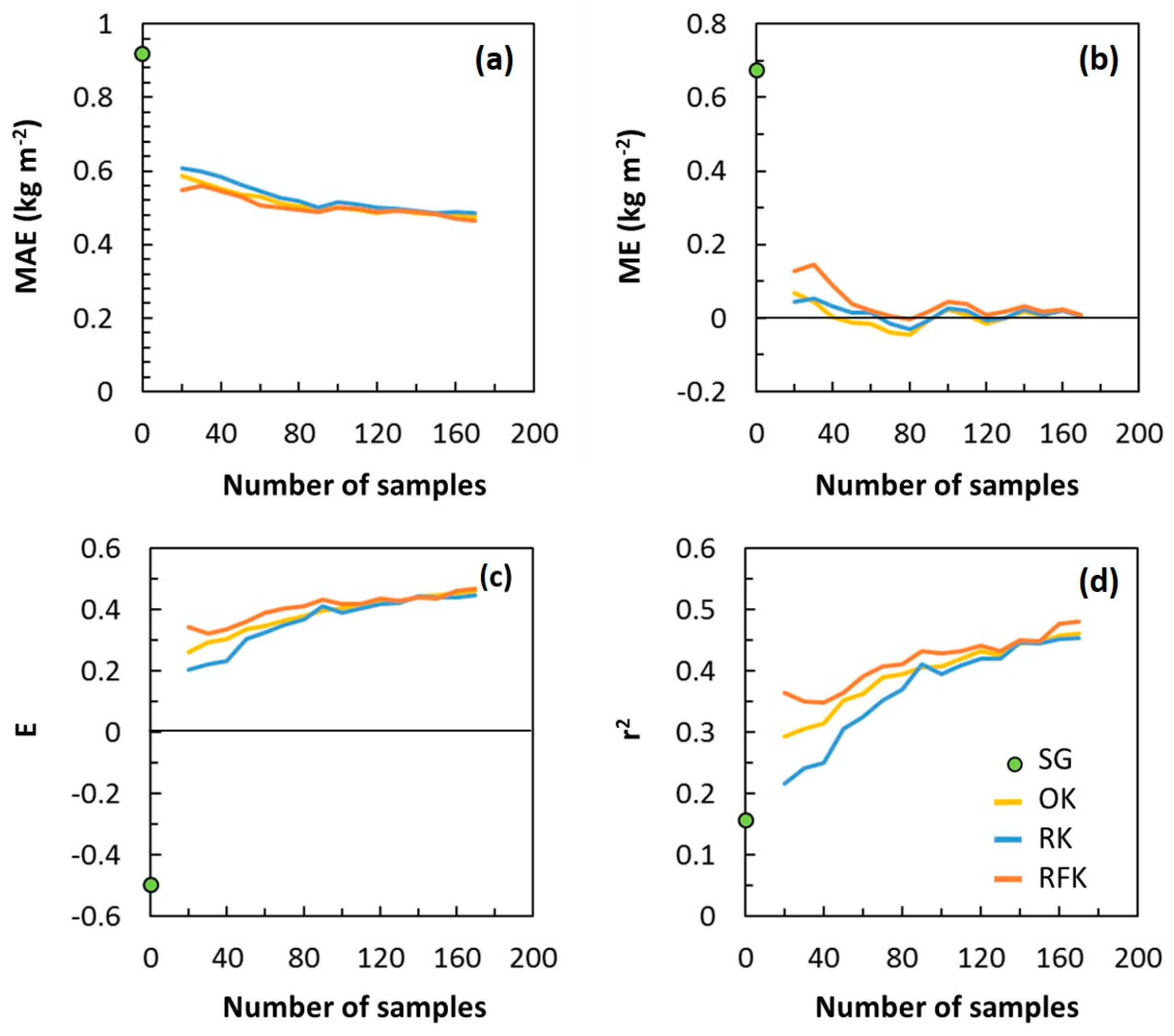
3.4. Map Accuracy versus Sampling Density

We plotted the four accuracy measures against the number of soil samples used to derive the baseline SOC stock map (Figure 4). The estimated accuracy measures are summarized in

Table 5. Evaluation measures for three of the sample sizes (n). SG = Soilgrids250m; OK = ordinary kriging; RK = regression kriging; RFK = random forest kriging, MAE = mean absolute error, ME = mean error, E = Nash-Sutcliffe modelling efficiency, and r² = the coefficient of determination for a linear regression model between predicted and observed values.

Method	N	MAE (kg m−2)	ME (kg m−2)	E	r2
SG	0	0.9	0.7	−0.49	0.16
OK	20	0.6	0.1	0.26	0.29
RK	20	0.6	0.0	0.20	0.22
RFK	20	0.5	0.1	0.34	0.36
OK	100	0.5	0.0	0.41	0.41
RK	100	0.5	0.0	0.39	0.40
RFK	100	0.5	0.0	0.42	0.43
OK	170	0.5	0.0	0.46	0.46
RK	170	0.5	0.0	0.45	0.46
RFK	170	0.5	0.0	0.47	0.48

. In all cases, local adaptation (Tier 4) improved the SOC stock baseline maps compared to using SG without correction (Tier 1). The difference between the three methods using local soil samples (OK, RK, and RFK) was, in general, small but for small sample sizes (≲100 samples) there was a gain in accuracy using the covariate stack (the RFK method) over creating a SOC stock baseline map by soil samples alone (OK) or in combination with the SG SOC stock map (RK). Kriging of the regression residuals and then adding these to the linear regression prediction did not, in this case, generate any consistent improvement over OK. Instead the RK method was often less accurate than the OK method. Presumably, because the SG map made a poor covariate.

The SG map overestimated the SOC stock in Otjozondjupa, but the positive bias (ME) could be rectified even by a small set of soil samples (≲60). The SG map itself was less accurate than the regional mean calculated from all soil samples (E < 0), while even a map made by OK of 20 samples was an improvement over the regional mean (E > 0). There was, however, a positive linear relationship (r = 0.38) between the SG map and the observed values at the sampling locations, and the negative E value of the SG maps was mainly due to the bias.

3.5. Maps

Figure 5 shows SOC stock baseline maps of the Otjozondjupa region created by different methods using different numbers of local samples. The original SoilGrids250m map is less smooth than the other maps; it shows a speckled, small-scale variation pattern. The general pattern with the lowest areas in the eastern part, and higher values in the west and northwest, is evident in all maps. In the mid-central part there is also an area of high values, something not captured with RK mapping. In the southwest, almost no samples were collected (Figure 4), and this is the area where the maps differ most; in some cases the area was mapped as having low SOC stock whereas the RFK maps indicated that SOC stock is high in that part. One can note that the maps derived from 170 local samples show different spatial variation structures depending on the method (OK, RK, or RFK) even though the evaluation statistics (Figure 6) indicate that they are about as accurate. The maps also show that RK and RFK produce spatial patterns that are more consistent across different sampling sizes than OK. RK and RFK, therefore, seem to be more robust predictors, i.e., depending less on the sampling configuration, than OK.

4. Discussion

4.1. Map Accuracy vs. Cost Considerations

It is self-evident that an increase in sampling points and, thus, cost, results in better map accuracy. The question is: at which point is the diminishing marginal increase in accuracy too costly? The present results indicate that with only a limited number of samples available, e.g., fewer than 60, it would be better to invest resources in using a more complex method to obtain better results. However, with an increasing number of samples, the difference in accuracy between the methods is relatively small. Given the high cost of soil sampling in the Otjozondjupa region it would, therefore, be best to sample between 80 and 100 locations and use the more complex RFK method. In a different region where the sampling cost is lower, it may be a better investment to collect more soil samples and use a less complex and costly method that does not have a high data preparation cost.

We include time requirements for different tasks in Table 4 and we assume that practitioners are familiar with the different DSM methods. By providing the time requirement in addition to the costs, a more accurate estimate of the total cost can be obtained which includes staff costs in different contexts. Given that Otjozondjupa is a large, sparsely-populated region with few roads and a high number of fenced private ranges, the data collection costs were relatively high.

4.2. Local Adaptation of Large-Extent Maps

It has been demonstrated that large-extent soil maps can be locally improved by the use of local soil observation data. For example, Malone et al. [58] first downscaled the SOC layer of the soil and landscape grid of Australia [59] to a finer grid by use of a set of high-resolution environmental covariates (Dissever method; originally described by Malone et al. [60]) and subsequently extended by Roudier et al. [61]. Then they adapted the downscaled map—that was rather biased—by use of local SOC observations for one test farm. By using residual kriging, Söderström et al. [62] tested local adaptation of the SOC and pH layers of the AfSoilgrids250m, an earlier version of Soilgrids250m covering the African continent [63], for the country of Rwanda. Similarly, Söderström et al. [64] updated a national soil texture map of Sweden [65] by re-parameterization of a MARSplines model that was used for prediction with local samples (farm extent) added to the calibration dataset, according to the principles of spiking [66]. In all cases the large-extent maps were improved by local adaptation. From the user´s perspective, regression kriging may be preferred over re-parameterization of the model used to derive the original map, since it does not require access to the data and models used to derive the original map. Local adaptation by regression kriging can also be performed directly without need for any harmonization of different soil sample datasets [42].

The results from the present study in a region of Namibia showed that using local samples (Tier 3) was better than using the global Soilgrids250m data (Tier 1), due to a severe bias of the global data. This was true whether the soil samples were used alone (OK) (Tier 3), in combination with the global soil dataset (RK) (Tier 4), or in combination with a large set of environmental covariate layers (RFK) (Tier 4). This bias in the SoilGris250m SOC stock map can be explained by the fact that the SoilGrids250m maps were developed using a global model and global datasets of (legacy) sample data and covariate layers. The global model does give unbiased predictions at global level given the input data, but this does not necessarily mean that, at the local level, there is no systematic difference between the mapped values and measured values. Furthermore, SoilGrids250m relies, to a large extent, on legacy sampling data, which might be dated and of limited accuracy that can cause further discrepancies between mapped values and values measured recently. Additionally, sampling sites used to develop the SoilGrids250m maps are unevenly distributed across the global land area. Nevertheless, SoilGrids250m is designed as an updateable mapping system that allows maps to improve over time when new datasets become available. Adding local data, such as the Otjozondjupa data to the SoilGrids250m sample dataset, might help to improve predictions for this region. Although digital soil maps of global, continental, or national extent may be invaluable as decision supports at the spatial scales for which they were intended, it shall not be taken for granted that such large-scale digital soil mapping products are relevant and directly applicable in smaller areas, such as a region, village, or farm [58,62].

4.3. Model Complexity and Costs

It is assumed that the degree of difficulty increases to implement and interpret the results from SG to OK, RK, and RFK. Local capacity, therefore, needs to be taken into consideration when evaluating which method to use in a given setting. For the more complex (higher tier) methods, training may be required. While the Otjozondjupa SOC baseline map was primarily produced by a team of international scientists, led by ISRIC, a subsequent SOC baseline is currently being produced by national technical staff who received two weeks of training. This investment will likely pay off for Namibia as the national capacity continues to grow and no additional training cost will be incurred with each subsequent sub-national baseline production or future monitoring.

The dilemma that decision-makers face in producing SOC baseline maps is whether to invest financial resources in collecting more samples and using a less complex method, or invest in building technical capacity in order to use a more complex method while collecting fewer samples, both approaches resulting in similar accuracy. Local decision-makers often want more autonomy over developing national LDN baselines and monitoring systems, and therefore tend to invest in technical capacity when possible. While this strategy can pay off in terms of having capacity that can be used in multiple ways, also beyond LDN, the risk is turnover and the resulting cost of training new staff. Therefore, when investing in technical capacity it is desirable to invest in redundancy by having more people trained in GIS, statistics, and programming than is required.

4.4. Recommendations

An obvious recommendation based on the present study, and also other literature, is to always take, at least a few, local soil samples, because (i) without local samples you will not know the accuracy of the global (or other large-extent) digital soil mapping product in your specific area of interest; and (ii) even a small set of local samples will help correct for a potential bias of the large-scale DSM product and thereby gain a great deal in accuracy for a relatively small cost.

Automatized web applications might be an option for this type of mapping. Even more complicated digital soil mapping functions using built-in prepared covariate layers can reduce labor costs and assist in the production of LDN baseline SOC stock maps of high accuracy. If interactive functionality is added, already a small number of national soil samples can be added to improve the modelling output. There is a working example of such an interactive web application for uploading soil sample data (at the farm level) which adapts a national scale digital soil map in Sweden [42], showing that such a solution is a feasible approach. Designing soil sampling based on the built-in covariates could be another function of such an application. Finally, a lesson learned from this (and other) studies is to take accessibility into account when designing the sampling.

4.5. General Validity of the Results

The present study was conducted in one region and the specific results cannot be regarded as pertinent for any area. However, we do believe that the following observations are general and also valid in other areas: (i) soil samples (even a few) improves large-scale maps (because possible local bias is removed); (ii) more local samples mean a better map and the increase in accuracy follows an increasing (concave down) shape showing diminishing returns; and (iii) the use of environmental covariates means a relatively larger improvement in accuracy when small sample sizes are used. For sufficiently large sample sizes, the added value of using covariates becomes less.

The finding that it is better to invest in soil samples than in salary for a well-trained data analyst using a more sophisticated mapping method is case-specific. Many countries would rather invest more in local capacity-building to increase in-house expertise which will pay dividends over a longer period. Nevertheless, the Otjozondjupa region is rather homogeneous and the dominating large-scale spatial variation patterns can easily be captured by taking a reasonable number of soil samples. In an area with more pronounced small-scale heterogeneity or in a patchy landscape with multiple land uses, the accuracy gain in using covariates is likely to be larger.

5. Conclusions

The lessons learned while developing the Otjozondjupa SOC baseline provide valuable insights for government departments that are responsible for developing LDN baselines elsewhere. The following observations made in the present study are considered general and can be used as a guide for planning LDN SOC stock baseline mapping:

(i)

taking a few local soil samples (e.g., 20) is necessary to assess the local accuracy of the large-scale map. The soil samples can also be used to alleviate local bias of the large scale map;

(ii)

taking more local samples further improves the map accuracy. The improvement will generally be smaller for each additional sample taken;

(iii)

using relevant environmental covariates will most likely improve the baseline SOC stock map. A relatively larger improvement in accuracy can be expected when soil sampling densities are used; and

(iv)

taking accessibility into account when designing the sampling can considerably save costs and labor in some areas.

The presented cost estimation for different DSM methods and sample sizes can be used as a budget template for new areas, but the amounts must be updated for the new context in which it is applied.

In the specific area of Otjozondjupa, Soilgrids250m generally overestimated the SOC stock in the upper 0.3 m of the soil profile in the Otjozondjupa region of Namibia. By using data from as few as 20 local soil samples, the Soilgrids250m map could be improved considerably. Using the local soil sample data to re-parameterize the random forest model was found to be the best option, statistically, but the improvement from using this more complex method compared to simply interpolating the soil sample data by ordinary kriging was minimal.

References

1. Food and Agriculture Organization (FAO). The State of the World’s Land and Water Resources for Food and Agriculture (SOLAW)—Managing Systems at Risk; Food and Agriculture Organization of the United Nations: Rome, Italy; Earthscan: London, UK, 2011; ISBN 978-1-84971-326-9. [Google Scholar]
2. Lal, R.; Safriel, U.; Boer, B. Zero Net Land Degradation: A New Sustainable Development Goal for Rio+20; United Nations Convention to Combat Desertification (UNCCD): Paris, France, 2012. [Google Scholar]
3. United Nations Convention to Combat Desertification (UNCCD). Report of the Conference of the Parties on Its 12th Session, Ankara, 12–23 October 2015. Available online: https://www2.unccd.int/official-documents/cop-12-ankara-2015 (accessed on 24 April 2018).
4. ELD Initiative. The Value of Land: Prosperous Lands and Positive Rewards through Sustainable Land Management. 2015. Available online: https://reliefweb.int/report/world/value-land-prosperous-lands-and-positive-rewards-through-sustainable-land-management (accessed on 24 April 2018).
5. Vlek, P.L.G.; Khamzina, A.; Tamene, L. Land Degradation and the Sustainable Development Goals: Threats and Potential Remedies. 2017. Available online: http://hdl.handle.net/10568/81313 (accessed on 24 April 2018).
6. The Montpellier Panel. No Ordinary Matter: Conserving, Restoring and Enhancing Africa’s Soils. 2014. Available online: https://ag4impact.org/wp-content/uploads/2014/12/MP_0106_Soil_Report_LR1.pdf (accessed on 23 March 2018).
7. United Nations Convention to Combat Desertification (UNCCD). Submission by the United Nations Convention to Combat Desertification on Decision 6/CP.17. 2011. Available online: http://unfccc.int/resource/docs/2012/smsn/igo/99.pdf (accessed on 23 March 2018).
8. Kust, G.; Andreeva, O.; Cowie, A. Land Degradation Neutrality: Concept development, practical applications and assessment. J. Environ. Manag. 2017, 195, 16–24. [Google Scholar] [CrossRef] [PubMed]
9. Grainger, A. Is Land Degradation Neutrality feasible in dry areas? J. Arid Environ. 2015, 112, 14–24. [Google Scholar] [CrossRef]
10. Stavi, I.; Lal, R. Achieving Zero Net Land Degradation: Challenges and opportunities. J. Arid Environ. 2015, 112, 44–51. [Google Scholar] [CrossRef]
11. Orr, B.J.; Cowie, A.L.; Castillo Sanchez, V.M.; Chasek, P.; Crossman, N.D.; Erlewein, A.; Louwagie, G.; Maron, M.; Metternicht, G.I.; Minelli, S.; et al. Scientific Conceptual Framework for Land Degradation Neutrality. A Report of the Science-Policy Interface. United Nations Convention to Combat Desertification (UNCCD), 2017. Available online: https://www2.unccd.int/publications/scientific-conceptual-framework-land-degradation-neutrality-report-science-policy (accessed on 24 April 2018).
12. Cowie, A.; Orr, B.; Castillo Sanchez, V.M.; Chasek, P.; Crossman, N.D.; Erlewein, A.; Louwagie, G.; Maron, M.; Metternicht, G.I.; Minelli, S.; et al. Land in balance: The scientific conceptual framework for Land Degradation Neutrality. Environ. Sci. Policy 2018, 79, 25–35. [Google Scholar] [CrossRef]
13. Chasek, P.; Safriel, U.; Shikongo, S.; Fuhrman, V.F. Operationalizing Zero Net Land Degradation: The next stage in international efforts to combat desertification? J. Arid Environ. 2015, 112, 5–13. [Google Scholar] [CrossRef]
14. Akhtar-Schuster, M.; Stringer, L.C.; Erlewein, A.; Metternicht, G.; Minelli, S.; Safriel, U.; Sommer, S. Unpacking the concept of land degradation neutrality and addressing its operation through the Rio Conventions. J. Environ. Manag. 2017, 195, 4–15. [Google Scholar] [CrossRef] [PubMed]
15. United Nations Convention to Combat Desertification (UNCCD). Land Degradation Neutrality Target Setting—A Technical Guide. 2016. Available online: http://www2.unccd.int/ldn-target-setting-technical-guide (accessed on 23 March 2018).
16. Smith, J. Towards Achieving Land Degradation Neutrality: Turning the Concept into Practice Project Evaluation: Final Report. UNCCD, Global Mechanism, 2015. Available online: http://www2.unccd.int/sites/default/files/relevant-links/2017-01/LDN%20project%20evaluation%20formatted%20report_0.pdf (accessed on 23 March 2018).
17. Aynekulu, E.; Lohbeck, M.; Nijbroek, R.; Ordóñez, J.C.; Turner, K.G.; Vågen, T.; Winowiecki, L. Review of Methodologies for Land Degradation Neutrality Baselines: Sub-National Case Studies from Costa Rica and Namibia. 2017. Available online: http://hdl.handle.net/10568/80563 (accessed on 23 March 2018).
18. Namibia Statistics Agency. Namibia 2011 Population and Housing Census Main Report. 2011. Available online: https://cms.my.na/assets/documents/p19dmn58guram30ttun89rdrp1.pdf (accessed on 25 April 2018).
19. Ministry of Environment and Tourism, Republic of Namibia. Namibia—Land Degradation Neutrality National Report 2015. 2015. Available online: https://knowledge.unccd.int/sites/default/files/inline-files/namibia-ldn-country-report-updated-version2.pdf (accessed on 24 April 2018).
20. Gilolmo, P.; Lobo, A. On the Relationship between Land Tenure and Land Degradation. A Case Study in the Otjozondjupa Region (Namibia) Based on Satellite Data. 2016. Available online: https://www.iss.nl/sites/corporate/files/43-ICAS_CP_Gilolm_and_Lobo.pdf (accessed on 23 March 2018).
21. Zeidler, J.; Kandjinga, L.; David, A. Study on the Effects of Climate Change in the Cuvelai Etosha Basin and Possible Adaptation Measures; Integrated Environmental Consultants of Namibia (IECN): Windhoek, Namibia; Integrated Environmental Consultants Namibia: Windhoek, Namibia, 2010; Available online: http://www.the-eis.com/data/literature/Climate%20Change%20in%20Cuvelai%20Etosha%20Basin%202010.pdf (accessed on 24 April 2018).
22. Global Mechanism of the UNCCD. Methodological Note to Set National Voluntary Land Degradation Neutrality (LDN) Targets Using the UNCCD Indicator Framework. 2016. Available online: http://www2.unccd.int/actions/ldn-target-setting-programme/ldn-methodological-note (accessed on 23 March 2018).
23. Hengl, T.; Mendes de Jesus, J.S.; Heuvelink, G.B.M.; Ruiperez Gonzalez, M.; Kilibarda, M.; Blagotić, A.; Shangguan, W.; Wright, M.N.; Geng, X.; Bauer-Marschallinger, B.; et al. SoilGrids250m: Global gridded soil information based on machine learning. PLoS ONE 2017, 12, e0169748. [Google Scholar] [CrossRef] [PubMed]
24. Burrough, P.A.; McDonnell, R.A. Principles of GIS; Oxford University Press: London, UK, 1998; ISBN 9780198742845. [Google Scholar]
25. Olsson, D.; Söderström, M. An automated method to locate optimal soil sampling sites using ancillary data. In Proceedings of the 4th European Conference on Precision Agriculture, Berlin, Germany, 15–17 June 2003. [Google Scholar]
26. Wetterlind, J.; Stenberg, B.; Söderström, M. The use of near infrared (NIR) spectroscopy to improve soil mapping at the farm scale. Precis. Agric. 2008, 9, 57–69. [Google Scholar] [CrossRef]
27. Sims, J.R.; Haby, V.A. Simplified colorimetric determination of soil organic matter. Soil Sci. 1971, 112, 137–141. [Google Scholar] [CrossRef]
28. Walkley, A.; Black, I.A. An examination of the Degtjareff method for determining soil organic matter, and a proposed modification of the chromic acid titration method. Soil Sci. 1934, 37, 131–137. [Google Scholar] [CrossRef]
29. Arrouays, D.; McKenzie, N.; Hempel, J.; Richer de Forges, A.C.; McBratney, A.B. GlobalSoilMap: Basis of the Global Spatial Soil Information System; CRC Press/Balkema: London, UK, 2014; ISBN 9781138001190. [Google Scholar]
30. De Brogniez, D.; Ballabio, C.; Stevens, A.; Jones, R.J.A.; Montanarella, L.; van Wesemael, B. A map of the topsoil organic carbon content of Europe generated by a generalized additive model. Eur. J. Soil Sci. 2015, 66, 121–134. [Google Scholar] [CrossRef]
31. Minasny, B.; McBratney, A.B. Digital soil mapping: A brief history and some lessons. Geoderma 2016, 264, 301–311. [Google Scholar] [CrossRef]
32. Stoorvogel, J.J.; Bakkenes, M.; Temme, A.J.; Batjes, N.H.; Brink, B.J. S-World: A Global Soil Map for Environmental Modelling. Land Degrad. Dev. 2017, 28, 22–33. [Google Scholar] [CrossRef]
33. Webster, R.; Oliver, M.A. Geostatistics for Environmental Scientists. Statistics in Practice, 2nd ed.; John Wiley & Sons Inc.: Chichester, UK, 2007; ISBN 978-0-470-02858-2. [Google Scholar]
34. Odeh, I.O.A.; McBratney, A.B.; Chittleborough, D.J. Further results on prediction of soil properties from terrain attributes-heterotopic co-kriging and regression kriging. Geoderma 1995, 67, 215–226. [Google Scholar] [CrossRef]
35. Hengl, T.; Heuvelink, G.B.M.; Rossiter, D.G. About regression-kriging: From equations to case studies. Comput. Geosci. 2007, 33, 1301–1315. [Google Scholar] [CrossRef]
36. Hengl, T.; Heuvelink, G.B.M.; Stein, A. A generic framework for spatial prediction of soil variables based on regression-kriging. Geoderma 2004, 120, 75–93. [Google Scholar] [CrossRef]
37. Sreenivas, K.; Dadhwal, V.K.; Kumar, S.; Harsha, G.S.; Mitran, T.; Sujatha, G.; Suresh, G.J.R.; Fyzee, M.A.; Ravisankar, T. Digital mapping of soil organic and inorganic carbon status in India. Geoderma 2016, 269, 160–173. [Google Scholar] [CrossRef]
38. Taghizadeh-Mehrjardi, R.; Nabiollahi, K.; Minasny, B.; Triantafilis, J. Comparing data mining classifiers to predict spatial distribution of USDA-family soil groups in Baneh region, Iran. Geoderma 2015, 253–254, 67–77. [Google Scholar] [CrossRef]
39. Breiman, L. Random forests. Mach. Learn. 2001, 45, 5–32. [Google Scholar] [CrossRef]
40. Hastie, T.; Tibshirani, R.; Friedman, J. The Elements of Statistical Learning. Data Mining, Inference, and Prediction, 2nd ed.; Springer Series in Statistics; Springer: New York, NY, USA, 2008; ISBN 978-0-387-84858-7. [Google Scholar]
41. Strobl, C.; Malley, J.; Tutz, G. An Introduction to Recursive Partitioning: Rationale, Application, and Characteristics of Classification and Regression Trees, Bagging, and Random Forests. Psychol. Methods 2009, 14, 323–348. [Google Scholar] [CrossRef] [PubMed] [Green Version]
42. Piikki, K.; Söderström, M.; Stadig, H. Local adaptation of a national digital soil map for use in precision agriculture. Adv. Anim. Biosci. 2017, 8, 430–432. [Google Scholar] [CrossRef]
43. Janssen, P.H.M.; Heuberger, P.S.C. Calibration of process-oriented models. Ecol. Model. 1995, 831, 55–66. [Google Scholar] [CrossRef]
44. Nash, J.E.; Sutcliffe, J.V. River flow forecasting through conceptual models part I—A discussion of principles. J. Hydrol. 1970, 103, 282–290. [Google Scholar] [CrossRef]
45. Krause, P.; Boyle, D.P.; Brau, F. Comparison of different efficiency criteria for hydrological model assessment. Adv. Geosci. 2005, 5, 89–97. [Google Scholar] [CrossRef]
46. Pebesma, E. Multivariable geostatistics in S: The gstat package. Comput. Geosci 2004, 30, 683–691. [Google Scholar] [CrossRef]
47. Gräler, B.; Pebesma, E.; Heuvelink, G. Spatio-Temporal Interpolation using gstat. R J. 2016, 8, 204–218. [Google Scholar]
48. Wickham, H. The Split-Apply-Combine Strategy for Data Analysis. J. Stat. Softw. 2011, 40, 1–29. [Google Scholar] [CrossRef]
49. Hijmans, R. raster: Geographic Data Analysis and Modeling. R Package Version 2.5-8. 2016. Available online: https://CRAN.R-project.org/package=raster (accessed on 24 April 2018).
50. Bivand, R.; Keitt, T.; Rowlingson, B. rgdal: Bindings for the Geospatial Data Abstraction Library. R Package Version 1.2-5; 2016; Available online: https://CRAN.R-project.org/package=rgdal (accessed on 23 March 2018).
51. Pebesma, E.; Bivand, R. Classes and methods for spatial data in R. R News 2005, 5, 9–13. [Google Scholar]
52. Bivand, R.; Pebesma, E.; Gomez-Rubio, V. Applied Spatial Data Analysis with R, 2nd ed.; Springer: New York, NY, USA, 2013; ISBN 9781461476177. [Google Scholar]
53. Baddeley, A.; Rubak, E.; Turner, R. Spatial Point Patterns: Methodology and Applications with R; Chapman and Hall; CRC Press: London, UK, 2015; ISBN 9781482210200. [Google Scholar]
54. Liaw, A.; Wiener, M. Classification and Regression by randomForest. R News 2002, 2, 18–22. [Google Scholar]
55. Kuhn, M. Caret: Classification and Regression Training. R Package Version 6.0-73. 2016. Available online: https://CRAN.R-project.org/package=caret (accessed on 23 March 2018).
56. Hengl, T. GSIF: Global Soil Information Facilities. R Package Version 0.5-3. 2016. Available online: https://CRAN.R-project.org/package=GSIF 01-1315 (accessed on 23 March 2018).
57. Nijbroek, R.; Mutua, J.; Söderström, M.; Piikki, K.; Kempen, B.; Hengari, S. Pilot Project Land Degradation Neutrality (LDN), Namibia: Establishment of a Baseline for Land Degradation in the Region of Otjozondjupa. 2017. Available online: https://cgspace.cgiar.org/handle/10568/80090 (accessed on 24 April 2018).
58. Malone, B.P.; Styc, Q.; Minasny, B.; McBratney, A.B. Digital soil mapping of soil carbon at the farm scale: A spatial downscaling approach in consideration of measured and uncertain data. Geoderma 2016, 290, 91–99. [Google Scholar] [CrossRef]
59. Grundy, M.J.; Rossel, R.A.V.; Searle, R.D.; Wilson, P.L.; Chen, C.; Gregory, L.J. Soil and landscape grid of Australia. Soil Res. 2015, 53, 835–844. [Google Scholar] [CrossRef]
60. Malone, B.P.; McBratney, A.B.; Minasny, B.; Wheeler, I. A general method for downscaling earth resource information. Comput. Geosci. 2012, 41, 119–125. [Google Scholar] [CrossRef]
61. Roudier, P.; Malone, B.P.; Hedley, C.B.; Minasny, B.; McBratney, A.B. Comparison of regression methods for spatial downscaling of soil organic carbon stocks maps. Comput. Electron. Agric. 2017, 142, 91–100. [Google Scholar] [CrossRef]
62. Söderström, M.; Piikki, K.; Cordingley, J. Improved usefulness of continental soil databases for agricultural management through local adaptation. S. Afr. J. Plant. Soil 2017, 34, 35–45. [Google Scholar] [CrossRef]
63. Hengl, T.; Heuvelink, G.B.M.; Kempen, B.; Leenaars, J.G.B.; Walsh, M.G.; Shepherd, K.D.; Sila, A.; MacMillan, R.; de Jesus, J.M.; Tamene, L.; et al. Mapping soil properties of Africa at 250 m resolution: Random forests significantly improve current predictions. PLoS ONE 2015, 10, e0125814. [Google Scholar] [CrossRef] [PubMed]
64. Söderström, M.; Sohlenius, G.; Rodhe, L.; Piikki, K. Adaptation of regional digital soil mapping for precision agriculture. Precis. Agric. 2016, 17, 588–607. [Google Scholar] [CrossRef]
65. Piikki, K.; Söderström, M. Digital soil mapping of arable land in Sweden–Validation of performance at multiple scales. Geoderma 2017, in press. [Google Scholar] [CrossRef]
66. Wetterlind, J.; Stenberg, B. Near infrared spectroscopy for within field soil characterisation—Small local calibrations compared with national libraries augmented with local samples. Eur. J. Soil Sci. 2010, 61, 823–843. [Google Scholar] [CrossRef]
Figure 1. Dominating land use classes in the 105,000 km2 Otjozondjupa region in Namibia. The map was generated based on Landsat 8 data and 279 ground-truth observations collected during the field work. The regional capital Otjiwarongo is marked.
Sustainability 10 01610 g001
Figure 2. The standardized exponential variogram model parameterized by the SoilGrids250m data in Otjozondjupa.
Sustainability 10 01610 g002
Figure 3. Schematic overview of the cross evaluation design with five folds and sixteen data subsets. In the left part (1) of the illustration, data in the orange folds were pooled, and for each of the five runs, sixteen data subsets of different sizes (20, 30, …, 170 observations) were used for mapping (using three different mapping methods). The right part (2) of the figure shows one run.
Sustainability 10 01610 g003
Figure 4. Map of planned sample locations and samples that were finally collected and analyzed in the Otjozondjupa region.
Sustainability 10 01610 g004
Figure 5. SOC stock maps of the Otjozondjupa region produced with different sample numbers and methods.
Sustainability 10 01610 g005
Figure 6. (a) Mean absolute error (MAE); (b) mean error (ME); (c) Nash-Sutcliffe modelling efficiency (E); and (d) the coefficient of determination (r2) for a linear regression model between predicted and observed values. The evaluation measures are plotted in relation to the number of samples used to derive the SOC stock baseline maps. The legend is valid for all four plots. SG = Soilgrids250m; OK = ordinary kriging; RK = regression kriging; and RFK = random forest.
Sustainability 10 01610 g006