Analysis of Regional Difference and Spatial Influencing Factors of Human Settlement Ecological Environment in China

Abstract

The importance of regions in shaping sustainable economic growth trajectories has been the subject of extensive research in recent years. When sustainable growth has been investigated in developing countries, a particular focus has been on China’s unsustainable development approach, which is characterized by high energy consumption and high pollution. Crucially, most of the research so far has focused on topics concerning ecological environment improvement. However, little is known regarding how the quality of human settlements environment can be accurately measured in terms of the concept of strong sustainability at the regional level. This study investigated human settlement environmental quality across 30 provinces in China from the perspective of strong sustainability and attempts to shed light on its spatial influence factors. Estimates are presented using a projection pursuit method. The results reveal that the quality of human settlement ecological environment declined over the period 2002–2014 with a significant geographical disparity in index performance. The results also suggest an observable spatial effect. The energy structure, energy intensity, and environmental control in a province not only have significantly positive effects on ecological quality of a province itself, but also bring spillover effects on its neighboring provinces. These three factors are also important in determining human settlement ecological quality in China.

1. Introduction

Human settlement ecological environment (hereinafter referred to briefly as HSEE) refers to the human living environment, which is an inclusive and open space for human life and development, and it is the most precious of human wealth. However, China has been facing a more severe living environment in recent years. According to the research on prevention and control of desertification (land degradation) in China, the average annual desertification losses reached 54 billion yuan [1]. Despite land disasters, 42% of China’s water systems are polluted, thus cannot be used for drinking, and even 36% of urban river water has already been rendered completely unusable [2]. At present, China’s economic development still heavily depends on high energy consumption and pollution, which is the main obstacle to the realization of sustainable development [3]. Severe resource constraints and continuous high-intensity industrial pollution, traffic pollution, and living pollution have deprived residents of a green living environment.

This contradiction between the increasing demand for a better living environment and the growing level of pollution has aroused the interest of a wide variety of researchers [4,5,6,7]. However, as one essential part of the research on HSEE, measuring its quality at the regional level is still in its infancy. So far, static studying is the main method employed, only considering HSEE quality in a certain year. As a result, dynamic patterns of economic development and pollution—particularly those related to the concept of sustainability—were essentially overlooked.

In this paper, we attempt to use the projection pursuit method to evaluate the HSEE quality across regions and provinces in China from the perspective of strong sustainability. According to the key research [8,9], HSEE can be defined as a complex ecosystem with a coordinated development of resources, environment, and society. This concept contains three basic parts: (1) the capacity of self-maintenance and regulation of the ecosystem (i.e., resilience of the ecosystem); (2) the supporting role of carrying media brought by social progress and economic development in the region; (3) the system pressure caused by resource loss and environmental pollution. Aiming to express features of the complex ecosystem in China, this study employed the theoretical framework of non-reductive total environmental welfare by considering the support index of nature.

Moreover, the scientific index system, which is suitable for sustainable development, is the theoretical foundation for evaluating HSEE. The purpose of evaluation is not to judge the quality of which province performs better, but to understand the internal operation mechanism of HSEE in China. The overall development is not a simple addition of the development across all subregions; instead, it relies on the harmonious relationship among single provinces. A province in China inevitably has spatial spillover effects on its neighboring economies through channels such as cross-border knowledge diffusion, technology spillover, and external effects of human capital, thus, identifying spillover effects is of positive significance for achieving coordinated and sustainable development. However, the existing research has not paid attention to the spatial impact on HSEE quality and has not distinguished direct and indirect consequences of the total spatial effect when considering the factors for improving HSEE in China. Therefore, based on quantitative methods, this paper measured and analyzed the regional differences in HSEE quality, and further decomposed the spatial effect to find ways to improve HSEE in China.

The research, from the perspective of strengthening HSEE, proved the validation of the integrative development framework. In comparison to past research, which only focused on testing the impact of multiple factors on environment quality, this paper introduces the concept of sustainability and further incorporates it with the existing theoretical framework. The research findings can be summarized as follows: (1) the HSEE quality in China declined integrally from 2002 to 2014; (2) regional differences in HSEE quality is significant, which largely depends on interregional and intraregional differences, and the fluctuation of HSEE quality by regions over time is comparatively stable; (3) HSEE exhibits spatial effects among provinces in China.

The remainder of this paper is organized as follows. The next section provides a literature review on HSEE. Section 3 sets out the methodological approaches employed. Section 4 and Section 5 contain the main results from varying perspectives, and Section 6 concludes the paper.

2. Literature Review

Geddes, Howard, and Mumfond have launched research to improve urban environment quality from different angles [10,11,12]. Doxiadis was the first to put forward the concept of “science of human settlements” [13], and he created a precedent of scientific research. Recently, theoretical study has been summarized as three categories, including city planning, residential enclaves, and ecology. With the development of society and economy, scholars paid more attention to studying influencing factors of HSEE, including human activities [14,15,16]; climate and environmental change [17]; soft environment social factors [18,19], and others.

Research of China’s human settlement environment has evolved from the perspectives of natural suitability study, comprehensive evaluation, and evolution of exploring, among other aspects. The measure of environmental quality is particularly noteworthy, as it is closely related to policy-making at present. For instance, Zhao et al. [5] constructed an index system from the natural environment and social economic environment, and they used a Back Propagation Neural network model to measure HSEE quality in five provincial capitals in northwestern China in 2005. Zhao et al. [20] set up an evaluation index system of HSEE in northeastern China cities from four aspects, including social economy, ecological environment, infrastructure services, and housing. They analyzed the temporal and spatial variation of HSEE using the Analytic Hierarchy Process method. The results show that spatial distribution of HSEE quality in northeastern China cities is overall stable. Based on climate data, land use data, and damage data, Sui [21] constructed an index system of HSEE using an analytic hierarchy process and the Delphi technique. Their results indicate that the chosen index system is suitable for the assessment of HESS in Shanghai. At the same time, scholars engaged in single factor evaluation. For example, Yang [22] assessed the suitability and restriction of the human settlement environment in Inner Mongolia using a single factor evaluation method, in terms of terrain, climate, and hydrology.

The above researches [20,21,22] used qualitative methods to measure HSEE. In addition to qualitative methods, the quality of ecological environments can be measured by quantitative methods. The qualitative evaluation selects an index that has a great impact on the ecological environment, and further evaluates ecological environment quality according to the number of the index or the degree of its merits and demerits. The quantitative evaluation adopts a certain formula or model to calculate the value of an index system, such as the ecosystem service value (ESV). There are a number of researchers who have tried their hand at measuring ESV in China, but they mainly focused on a specific region and single type of natural capital. For example, Chen et al. studied the ESV in the western mountain area of Henan province. Their results show that the ecological service value of Luanchuan increased dramatically from 2005 to 2010, then went back down to the level of 2005 in 2014 [23]. Combining regional difference, spatial heterogeneity, and differences in economic development level in different areas, Liu and Feng incorporated 12 high-performance indicators for the ecological services function to evaluate the ecological services value for alpine rangeland in the Naqu region of northern Tibet. The findings indicate that the total annual ecological services value of alpine rangeland was 119.907 billion RMB in the Naqu region, in which the ecological services value of alpine steppe, alpine desert, alpine desert steppe, and alpine meadow accounted for 62.9%, 1.5%, 8%, and 28.1% of the total ecological services value, respectively [24]. Based on the net primary productivity evaluation model and the ecological service value model, Liu et al. calculated net primary productivity, atmosphere adjustment value, water conservation value, soil and water conservation value, and environmental purity value in Shaanxi province and then analyzed its dynamic change. The results show that ESV of cultivated land rose again after a decline, from 2000 to 2009, with an increase of 20.537 billion yuan. The water conservation value possessed the largest proportion contribution of all ESV components, followed by the soil and water conservation value, and environmental purity value had the minimum proportion contribution [25].

The study of HSEE in China is not limited to quality evaluation but has expanded to diversity in space. Liu studied spatial differences of habitat environment quality of 13 cities in Jiangsu province [4]. He explored the causes of such differences using principal component analysis and system clustering analysis methods. Zhang studied regional differences of HSEE quality and expatiated on corresponding reasons [6]. Feng studied China’s habitat suitability of the ecological environment using GIS technology, and found that China’s settlement environmental quality showed a downward trend from the southeast coast to northwest inland [26]. Yang studied HSEE quality and its space differentiation pattern in Dalian, China. Using a spatial analysis method based on a geographic information system [27], he stated that the security unit of the ecological environment of Dalian can be divided into five phases, from optimal to worse. Li discussed spatial differences of China’s HSEE quality through an entropy weight method and found HSEE quality and economic development were positively correlated [28]. In addition, authors have also studied HSEE at the regional level, but mainly focused on analyzing space differences in key areas of China, such as in Pearl River delta [29], Bohai area [30], northeast of China [31], Liaoning province (Li, 2014) [32], and others.

As discussed above, scholars’ attention to the HSEE in China encouraged fruitful achievements in relevant research fields [26,27,28,29,30,31,32]. However, few scholars have focused on measuring HSEE quality across provinces. On the contrary, they have frequently considered a certain region, such as a province or a city. Many researches also focused too much on static study, as the quality of HSEE was only measured in a certain year. Studying HSEE in China in one year cannot capture group variations over time and is likely to lead to biased judgment. Finally, the concept of sustainable development was essentially overlooked. It has been frequently used to understand the shift in growth towards a more sustainable approach. Pearce divided sustainable development into strong sustainability and weak sustainability [33]. The weak sustainability holds that single capital can be substituted by other capital [33], in other words, various types of capital are interchangeable. The weak sustainability just ensures that the general wealth is not reduced. However, the assumption of strong sustainability implies that the general natural capital is partly replaced, and the key natural capital cannot be replaced [33]. Therefore, according to the demand for non-decreasing development of environmental welfare in the theory of strong sustainability, the absorptive (self-purification) capacity of the environment has to be constantly improved for maintaining the non-reduction of the total environmental welfare if there is damage to the ecological environment. Shuji etc. [34] showed that plants, soils, rivers, and wetlands can absorb and purify air pollution, water pollution, as well as solid pollutants. Thus, the capacity of environmental absorption (self-purification) also reflects the fact that human beings actively influence the ecological quality through the transformation of nature. Therefore, the lack of environmental absorption can easily result in the imbalance and distortion of the evaluation of HSEE.

In order to empirically bridge the gap between HSEE and sustainability research, this paper tries to develop a theoretical framework that integrates the perspective of strong sustainability for evaluating HSEE quality at the regional level in China. This paper also analyzes the main results from varying perspectives and attempts to shed light on spatial effects of HSEE in China’s provinces. The ecological environment is a system with the feature of comprehensiveness and complexity, which also involves many influencing factors. Such a dynamic and interpretational pattern, however, cannot be accurately captured by qualitative models (e.g., producing EVS). Therefore, using mathematical and econometric methods, the paper aims at measuring the quality of HSEE from an integrative perspective, rather than focusing on signal aspects separately.

3. Methods and Materials

3.1. Index System and Data Sources

Based on technical specifications for ecological environment evaluation issued by China’s Environmental Protection Administration, the ecological evaluation covers the biological abundance, vegetation cover, water density, land degradation, and environmental quality [35]. In addition, the “Evaluation Method for the Target of Ecological Civilization Construction”, implemented in 2016, highlights the principle of public sense of gain. We selected indexes, which distinguish the pressure index and support index, to measure HSEE. The list of indexes is shown in

Table 1. Index system.

	Index	Index Type
climate	average annual rainfall (mm)	neutral
	annual sunshine hours (h)	support
	annual average temperature (°C)	neutral
land	per capita area of cultivated farmland (hectares)	support
hydrology	surface water resources (cubic meters)	support
	ground water resources (cubic meters)	support
vegetation	vegetation cover rate	support
economy	GDP (10,000 yuan)	support
	proportion of tertiary industry	support
	open degree	support
	high-tech output value (10,000 yuan)	support
	energy consumption (10,000 tons of standard coal)	pressure
population	population density (10,000 people per hectare)	neutral
	urbanization rate	support
atmosphere	industrial waste gas (million standard cubic meters)	pressure
	sulfur dioxide (10,000 tons)	pressure
	carbon dioxide (million tons)	pressure
	smoke (powder) dust (10,000 tons)	pressure
water	wastewater emissions (million tons)	pressure
soil	industrial solid waste (tons)	pressure
	garbage collection capacity (10,000 tons)	pressure
	fertilizer application (10,000 tons)	pressure
	pesticide use (tons)	pressure

, which includes three categories: a higher value of support index, indicating a better HSEE quality; a higher value of pressure index, indicating a lower HSEE quality; and neutral indexes, which are important for determining HSEE quality but are maintained in a certain range.

A crucial point of the establishment of the index system is how the philosophy of “nature–society–environment” can be appropriately reflected within the composite system. The physical condition is the material basis of the system, which reflects the state of the system itself. According to Gao [8], the nature of the ecosystem is determined by the condition of climate, soil, landform, hydrology, and soil. Therefore, this study adopted a similar approach and measured the natural condition from four aspects: climate, land, hydrology, and vegetation cover. The landform is not included, as it is a static index. Concretely speaking, the measure of climate includes average annual rainfall, average annual sunshine hours, and average annual temperature; the measure of land is represented by per capita area of cultivated farmland; and the estimate of hydrology involves surface water resources and groundwater resources. These indicators reflect environmental self-purification capabilities, such as plants, soils, rivers, and wetlands, which (to a certain degree) have absorption and purification effects on different types of pollution (Tian et al. [31]). Therefore, the inclusion of the index meets the basic requirement of the theory of sustainable development mentioned above.

Economy aspects include GDP, the proportion of tertiary industry, open degree, high-tech output value, and energy consumption; population indicators include population density and urbanization rate.

To assess the impact of environment, most of studies only implemented a single factor analysis, using wastewater pollutant discharge [36], hazardous waste [37], and fine particulate matter [38] as indicators. Although these studies can describe the current situation of the environment from different angles, there is a lack of comprehensive description. Therefore, an additional useful extension was adopted for accounting for the integrative effect by measuring air, water, and soil together. Finally, the atmosphere dimension includes industrial waste gas, sulfur dioxide, smoke (powder) dust, carbon dioxide; the water dimension involves pollution wastewater emissions; and the soil dimension includes industrial solid waste, garbage collection capacity, fertilizer application, and pesticide use.

This study investigates the HSEE quality over the period 2002–2014. Datasets that were used in this study when generating variables at the regional level comprised China’s statistical yearbook, China’s environment statistical yearbook, and China’s rural statistical yearbook. Hong Kong, Macao, Taiwan, and Tibet were not included due to data constraints. It is worth mentioning that China has no official carbon dioxide emissions statistics presently, so this analysis calculated it. We divided energy consumption into nine categories, including raw coal, coke, crude oil, gasoline, kerosene, diesel oil, fuel oil, gas, and electricity, and then we calculated carbon dioxide emissions utilizing the standard coal conversion coefficient and coefficient of carbon emissions. (For the specific calculation method see “National Greenhouse Gas Emissions Inventory Guide”, IPCC (2006).)

3.2. Calculation Method

The projection pursuit (PP) method [39] was employed in the study for evaluating HSEE at the regional level in China. The projection pursuit method is driven directly by sample data. The method is especially suitable for processing nonlinear, non-normal, and high-dimensional data. Its basic idea is finding a projection, which allows the high-dimensional data to be represented by low-dimensional data.

Assuming $A=\{i=1~m\}$ denotes $m$ individual samples, $C=\left\{C_j\right|j=1~n\}$ denotes evaluation index set, $x_{ij}$ denotes value of index $C_j$ of individual $A_i$. Evaluation steps are as follows:

Step 1. Data normalization.

The step is to eliminate the different units and to unify change direction of indexes.

For constructing pressure index, let

$$y_{ij}=\frac{x_j^{\max }-x_{ij}}{x_j^{\max }-x_j^{\min }},i=1,2,\cdots ,m;j=1,2,\cdots ,n$$

(1)

For constructing support index, let

$$y_{ij}=\frac{x_{ij}-x_j^{\min }}{x_j^{\max }-x_j^{\min }},i=1,2,\cdots ,m;j=1,2,\cdots ,n$$

(2)

In Formulas (1) and (2), $x_j^{\max }$, $x_j^{\min }$ denote the maximal value and the minimum value of $j$ index, respectively.

For constructing neutral index, let

$$y_{ij}=1-\frac{\left|x_{ij}-x_j^{\ast }\right|}{\begin{array}{c}\max \\ i\end{array}\left|x_{ij}-x_j^{\ast }\right|},i=1,2,\cdots ,m;j=1,2,\cdots ,n$$

(3)

where, $x_j^{\ast }$ denotes optimal value or mean of $j$ index. In this study, we adopted the mean value.

Step 2. Constructing ecological environment evaluation function and projection index function.

$PP$ method synthesizes $n$ dimension data $\left\{y_{ij}\right|j=1~n\}$ to a projection value $Z_i$ with the projection direction $a=(a_1,a_2,\cdots ,a_n)$, namely

$$Z_i={\displaystyle \sum _{j=1}^n{a}_j}{y}_{ij},i=1,2,\cdots m;j=1,2,\cdots ,m$$

(4)

where $a$ is weight vector, $Z_i$ is ecological environment evaluation function of sample $i$, which portrays the ecological environment. A lower projection value represents a corresponding worse ecological environment. When $PP$ method synthesizes $Z_i$, it requires $Z_i$ have characteristics such that the local projection point is as dense as possible, while the overall projection groups are as spread as possible. Thus, the projection index function can be constructed as

$$Q(a)=S_z{D}_z$$

(5)

where $S_z$ is standard deviation of $Z_i$, $D_z$ is the local density of $Z_i$, namely

$$S_z=\sqrt{\frac{1}{m-1}{\displaystyle \sum _{i=1}^m{(Z_i-\overline{Z})}^2}}$$

(6)

$$D_z={\displaystyle \sum _{i=1}^m{\displaystyle \sum _{j=1}^m(R-r_{ij})I(R-r_{ij})}}$$

(7)

where $\overline{Z}=\frac{1}{m}{\displaystyle \sum _{i=1}^m{Z}_i}$ is the mean of $Z_i$; $R$ is the window radius for local density. The window radius should not only make the average number of projection points included in the window too small, avoiding large average deviation of the slide, but also should not make it increase too quickly with $m$ increasing.

Generally, $R$ is set as $0.1\times S_z$. $r_{ij}=\left|Z_i-Z_j\right|$; $I(t)$ is the indicator function; when $t<0$, it equals zero, otherwise, it equals one.

Step 3. Optimizing the projection index function.

When the sample set is given, the projection index function only changes with the projection direction. Different projection directions reflect different data structure characteristics, the best projection direction is the one that is most likely to expose some kind of characteristic structure of high-dimensional data. The optimal projection direction can be estimated by solving the problem of maximizing the projection function

$$\begin{array}{l}\max \mathrm{Q}(\mathrm{a})={\mathrm{S}}_{\mathrm{z}}{\mathrm{D}}_{\mathrm{z}}\\ s.t.{\displaystyle \sum _{j=1}^n{a}_j=1}\\ a_j>0(j=1,2,\cdots ,n)\end{array}$$

(8)

Actually, (8) is a complex nonlinear optimization problem with variables $\left\{a_j\right|j=1~n\}$. We solved it by genetic algorithm.

Step 4. Calculate HSEE quality index $Z_i$.

$$Z_i={\displaystyle \sum _{j=1}^n{a}_j}{y}_{ij},i=1,2,\cdots m;j=1,2,\cdots ,m$$

(9)

where the weight $a_j$ is obtained by PP method. The weight is determined by the variables generated from the actual data and is also time variant.

3.3. Regional Difference Analysis Method

The information entropy was utilized for measuring the difference for two reasons: the information entropy can not only judge the level of the whole difference, but also distinguish the intraregional and interregional differences; the values, obtained by information entropy, of different time and space can be directly compared. The calculation formula is as follows:

$$E=-{\displaystyle \sum _{i=1}^n{p}_i\log (p_i)}$$

(10)

Using the above formulas, the difference between regions or within regions can be further defined, as follows:

$$\begin{array}{cc}\hfill E=& -{\displaystyle \sum _{i=1}^n{p}_i\log (p_i)}=-{\displaystyle \sum _{k=1}^m{\displaystyle \sum _{i=1}^{n_k}\frac{p_i}{w}\log (\frac{p_i}{w})}}=-({\displaystyle \sum _{k=1}^m\frac{w_k}{w}{\displaystyle \sum _{i=1}^{n_k}\frac{p_i}{w_k}\log (\frac{p_i}{w_k})}}+\hfill \\ & {\displaystyle \sum _{k=1}^m\frac{w_k}{w}{\displaystyle \sum _{i=1}^{n_k}\frac{p_i}{w_k}\log (\frac{w_k}{w})}})={\displaystyle \sum _{k=1}^m\frac{w_k}{w}}E(k)+E(w)=E_I+E_M\hfill \end{array}$$

(11)

where $n$ is the sample number, which is divided into $m$ groups, group $k$ has $n_k$ samples, and its mean quality is $w_k$, the average value of all environmental quality indexes $w$. $p_i$ denotes quality index of individual $i$, $E_I$ denotes unequal weighting value of $m$ groups, with corresponding weight $\raisebox{1ex}{$w_k$}\!\left/ \!\raisebox{-1ex}{$w$}\right.$, and $E_M$ denotes difference between regions.

3.4. Basic Spatial Model

The spatial model includes spatial lag model, spatial error model, and spatial Dubin model. The spatial lag model (SLM) can be set as:

$$SQ{I}_{it}={\epsilon }_{it}+{\beta }_0{\displaystyle \sum _{j=1}^{31}{W}_{ij}}SQ{I}_{it}+{\beta }_{1}x{q}_{it}+{\beta }_{2}hjg{z}_{it}+{\beta }_{3}e{c}_{it}+{\beta }_{4}cit{y}_{it}+{\beta }_{5}lpgd{p}_{it}+{\beta }_{6}ed{u}_{it}+{\beta }_{7}e{n}_{it}$$

(12)

where $\epsilon$ denotes the error term, $W$ denotes spatial weight matrix, $SQI$ denotes the quality of HSEE.

The spatial error model (SEM) can be set as:

$$SQ{I}_{it}={\displaystyle \sum _{j=1}^{31}{W}_{ij}}{\epsilon }_{it}+{\xi }_{it}+{\beta }_{1}x{q}_{it}+{\beta }_{2}hjg{z}_{it}+{\beta }_{3}e{c}_{it}+{\beta }_{4}cit{y}_{it}+{\beta }_{5}lpgd{p}_{it}+{\beta }_{6}ed{u}_{it}+{\beta }_{7}e{n}_{it}$$

(13)

The spatial Dubin model (SDM) can be set as:

$$\begin{array}{l}SQ{I}_{it}=\alpha +{\lambda }_t+{\mu }_i+{\beta }_0{\displaystyle \sum _{j=1}^{31}{W}_{ij}}SQ{I}_{it}+{\beta }_{1}x{q}_{it}+{\beta }_{2}hjg{z}_{it}+{\beta }_{3}e{c}_{it}+{\beta }_{4}cit{y}_{it}+{\beta }_{5}lpgd{p}_{it}\\ +{\beta }_{6}ed{u}_{it}+{\beta }_{7}e{n}_{it}+{\theta }_1{\displaystyle \sum _{j=1}^{31}{W}_{ij}}x{q}_{it}+{\theta }_2{\displaystyle \sum _{j=1}^{31}{W}_{ij}}hjg{z}_{it}+{\theta }_3{\displaystyle \sum _{j=1}^{31}{W}_{ij}}e{c}_{it}+{\theta }_4{\displaystyle \sum _{j=1}^{31}{W}_{ij}}cit{y}_{it}+{\theta }_5{\displaystyle \sum _{j=1}^{31}{W}_{ij}}lpgd{p}_{it}\\ +{\theta }_6{\displaystyle \sum _{j=1}^{31}{W}_{ij}}ed{u}_{it}+{\theta }_7{\displaystyle \sum _{j=1}^{31}{W}_{ij}}e{n}_{it}+{\epsilon }_{it}\end{array}$$

(14)

The control variables are described below.

Foreign trade $\exp$: in order to eliminate the instability caused by price changes, we used the ratio of exports and GDP of each province to measure. Environmental control $er$: for characteristics of this study and data, we used the ratio of pollution control investment and industrial wastewater discharge as a measure of environmental regulation. Energy structure $ec$: measured by the ratio of raw coal consumption and total energy consumption. Energy intensity $en$: described by the ratio of GDP and total energy consumption. Urbanization level $city$: measured by the ratio of urban population to the total population. The level of economic development $lpgdp$: measured by the logarithm of actual per capita GDP; in order to eliminate the impact of prices, GDP is firstly processed by deflator reduction (1978 as the base period). Resident quality $edu$: measured by the per capita education level.

3.5. Spatial Effect Decomposition Method

LeSage and Pace [40] pointed out that using the point estimation method to test spillover effect of spatial variables is biased, so they proposed that the coefficient should be divided into direct effect and indirect effect, according to the source of the variable, by means of differentiation. The specific method is shown as follows.

In general, SDM can be expressed as

$$(I_n-\rho W)y=X\beta +X\beta \theta +{\iota }_n\alpha +\epsilon$$

(15)

$$y={\displaystyle \sum _{r=1}^k{S}_r}(W)x_r+V(W){\iota }_n\alpha +V(W)\epsilon$$

(16)

where $S_r(W)=V(W)(I_n{\beta }_r+W{\theta }_r),V(W)={(I_n-\rho W)}^{-1}=I_n+\rho W+{\rho }^{2}W+\cdots$

Rewritten in matrix form:

$$\left(\begin{array}{c}{y}_1\\ y_2\\ ⋮\\ y_n\end{array}\right)={\displaystyle \sum _{r=1}^k\left(\begin{array}{cccc}{S}_r{(W)}_{11}& S_r{(W)}_{12}& \cdots & S_r{(W)}_{1n}\\ S_r{(W)}_{21}& S_r{(W)}_{22}& \cdots & S_r{(W)}_{2n}\\ ⋮& ⋮& \cdots & ⋮\\ S_r{(W)}_{n1}& S_r{(W)}_{n2}& \cdots & S_r{(W)}_{nn}\end{array}\right)\left(\begin{array}{c}{x}_{1r}\\ x_{2r}\\ ⋮\\ x_{nr}\end{array}\right)}+V(W){\iota }_n\alpha +V(W)\epsilon$$

(17)

Generally, for individual $i$,

$$y_i={\displaystyle \sum _{r=1}^k[S_r{(W)}_{i1}{x}_{1r}}+S_r{(W)}_{i2}{x}_{2r}+\cdots +S_r{(W)}_{in}{x}_{nr}]+V{(W)}_i{\iota }_n\alpha +V{(W)}_i\epsilon$$

(18)

$\frac{\partial y_i}{\partial x_{ir}}=S_r{(W)}_{\mathit{ii}}$ represents average influence to $y$ created by $x$ in the region itself, namely, direct effect, with a value equal to the mean of diagonal elements of $S_r(W)$, expressed as

$$\overline{M}{(r)}_{direct}=n^{-1}trace(S_r(W));$$

(19)

$\frac{\partial y_i}{\partial x_{jr}}=S_r{(W)}_{ij}$ represents average influence to $y$ created by $x$ in other regions, namely, indirect effect, expressed as

$$\overline{M}{(r)}_{indirect}=\overline{M}{(r)}_{total}-\overline{M}{(r)}_{direct},$$

(20)

where total effect equals the mean of elements of $S_r(W)$, expressed as $\overline{M}{(r)}_{total}=n^{-1}{\iota }_n^{\prime }{S}_r(W){\iota }_n$.

4. Variation and Difference of HSEE in China

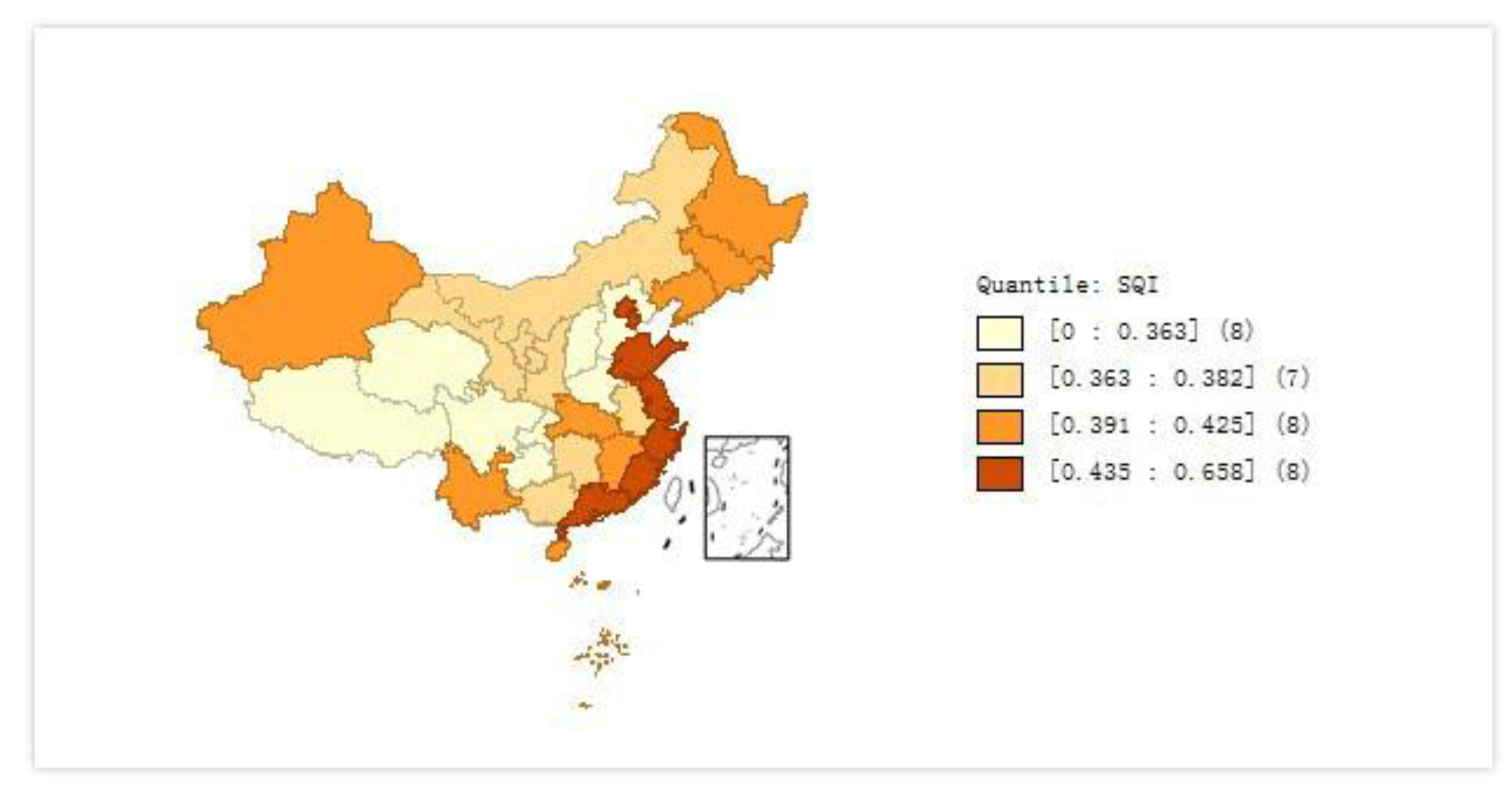
4.1. HSEE in Provinces

This section highlights findings from analyzing China’s HSEE in relation to the indexes listed in Table 1. The specific results are shown in

Table 2. Human settlement ecological environmental (HSEE) quality of China’s 30 provinces (2002–2014).

	2002	2003	2004	2005	2006	2007	2008	2009	2010	2011	2012	2013	2014
Beijing	0.5870	0.5856	0.6538	0.3642	0.4425	0.5050	0.4856	0.5460	0.5261	0.5612	0.4920	0.4357	0.4805
Tianjin	0.5001	0.5100	0.5242	0.3861	0.3876	0.4347	0.3891	0.4412	0.4518	0.4854	0.4442	0.4023	0.4381
Hebei	0.3711	0.3662	0.4502	0.2043	0.3571	0.3620	0.2944	0.3215	0.4089	0.3731	0.3568	0.3096	0.3348
Shanxi	0.2964	0.3804	0.4463	0.1870	0.2753	0.3217	0.2347	0.2744	0.3645	0.3641	0.3206	0.2871	0.3245
Neimenggu	0.4059	0.5072	0.5638	0.2297	0.3369	0.3950	0.2750	0.3163	0.4154	0.4250	0.3722	0.3414	0.3642
Liaoning	0.4289	0.4450	0.4884	0.3593	0.3870	0.4263	0.3394	0.3978	0.4539	0.4759	0.4401	0.4120	0.4692
Jilin	0.4963	0.5430	0.5620	0.3866	0.3612	0.4244	0.3170	0.3455	0.4209	0.4727	0.4035	0.3497	0.3966
Heilongjiang	0.4566	0.4790	0.5210	0.3572	0.3548	0.4120	0.3198	0.3462	0.4140	0.4375	0.3693	0.3495	0.3592
Shanghai	0.6164	0.5631	0.5869	0.4275	0.5642	0.5608	0.5798	0.6317	0.5462	0.5615	0.5650	0.5450	0.5527
Jiangsu	0.6805	0.5482	0.5327	0.4815	0.6250	0.5847	0.6161	0.6173	0.6238	0.6142	0.6545	0.6871	0.7086
Zhejiang	0.4951	0.4935	0.4798	0.4706	0.4667	0.4775	0.4710	0.4814	0.4870	0.4816	0.5011	0.4819	0.4701
Anhui	0.4146	0.4244	0.4432	0.4492	0.3461	0.3782	0.3128	0.3252	0.3845	0.4026	0.3822	0.3587	0.3479
Fujian	0.4850	0.5017	0.4965	0.4936	0.3960	0.4141	0.3930	0.3958	0.4025	0.4328	0.4295	0.4032	0.4096
Jiangxi	0.4152	0.5238	0.4910	0.6021	0.3313	0.4000	0.3190	0.3236	0.3853	0.4174	0.3781	0.3513	0.3411
Shandong	0.4363	0.4589	0.4476	0.5969	0.4914	0.4548	0.4271	0.4649	0.4991	0.4765	0.5035	0.5419	0.5680
Henan	0.3790	0.3311	0.3492	0.3479	0.3360	0.3455	0.2952	0.3083	0.3527	0.3426	0.3648	0.3546	0.3884
Hubei	0.4199	0.4136	0.4364	0.3795	0.3733	0.4160	0.3504	0.3501	0.3757	0.4150	0.4014	0.4117	0.3943
Hunan	0.3717	0.3915	0.3810	0.3521	0.3308	0.3687	0.3194	0.3158	0.3766	0.4000	0.3850	0.3800	0.3531
Guangdong	0.6239	0.6126	0.5441	0.5618	0.7100	0.6617	0.7261	0.6967	0.6506	0.6719	0.6965	0.7295	0.7419
Guangxi	0.3604	0.4523	0.3720	0.5613	0.2840	0.3403	0.2962	0.2822	0.3292	0.3860	0.3398	0.3232	0.2900
Hainan	0.4403	0.5056	0.5159	0.6992	0.3155	0.3627	0.3135	0.3262	0.3751	0.4042	0.3594	0.3061	0.3292
Chongqing	0.3386	0.3004	0.2611	0.4564	0.2657	0.3049	0.2958	0.2723	0.2733	0.3514	0.3355	0.3181	0.2577
Sichuan	0.3231	0.2928	0.2557	0.4599	0.3211	0.3251	0.3428	0.3192	0.2958	0.3615	0.3893	0.3924	0.3478
Guizhou	0.2103	0.2449	0.2272	0.5968	0.2050	0.2536	0.2405	0.2140	0.2283	0.2625	0.2556	0.2395	0.2048
Yunnan	0.4360	0.5233	0.5012	0.4524	0.3370	0.3912	0.3055	0.3157	0.3904	0.4049	0.3765	0.3363	0.3731
Shaanxi	0.3869	0.4024	0.4207	0.4349	0.3243	0.3692	0.2969	0.3092	0.3816	0.4155	0.3653	0.3475	0.3524
Gansu	0.4140	0.4964	0.5234	0.4016	0.3173	0.3571	0.2681	0.2901	0.4043	0.4092	0.3349	0.2976	0.3277
Qinghai	0.4267	0.5021	0.5081	0.3065	0.2948	0.3611	0.2578	0.2921	0.4189	0.4147	0.3385	0.2786	0.3158
Ningxia	0.4329	0.5160	0.5726	0.3190	0.3113	0.3708	0.2647	0.3066	0.4138	0.4106	0.3397	0.2833	0.3291
Xinjiang	0.4496	0.5384	0.5313	0.2918	0.3437	0.4145	0.2922	0.3273	0.4313	0.4434	0.3481	0.3164	0.3577

. (We have reason to believe that the indicator used in this paper is a good indicator of HSEE. On one hand, the indicators are constructed based on an objective concept including three basic elements: (1) the capacity of self-maintenance and regulation of the ecosystem (i.e., resilience of the ecosystem); (2) the supporting role of carrying media brought by social progress and economic development in the region; (3) the system pressure caused by resource loss and environmental pollution. On the other hand, the result of using the quality index is factual. As shown in

Table 3. Ranking of ecological environmental quality of China’s 30 provinces.

Province	Mean	Rank	Province	Mean	Rank	Province	Mean	Rank
Guangdong	0.6636	1	Xinjiang	0.3912	16	Shaanxi	0.3698	21
Jiangsu	0.6134	2	Anhui	0.3823	17	Hunan	0.3635	22
Shanghai	0.5616	3	Neimenggu	0.3806	18	Qinghai	0.3627	23
Beijing	0.5127	4	Ningxia	0.3746	19	Guangxi	0.3551	24
Shandong	0.4898	5	Gansu	0.3724	20	Hebei	0.3469	25
Zhejiang	0.4813	6	Jiangxi	0.4061	11	Henan	0.3458	26
Tianjin	0.4458	7	Hainan	0.4041	12	Sichuan	0.3405	27
Fujian	0.4349	8	Heilongjiang	0.3982	13	Shanxi	0.3136	28
Liaoning	0.4249	9	Yunnan	0.3957	14	Chongqing	0.3101	29
Jilin	0.4215	10	Hubei	0.3952	15	Guizhou	0.2602	30

, Guangdong tops the list of ranking, followed by Jiangsu, Shanghai, Beijing, Shandong, Zhejiang, Tianjin, and Fujian. The last eight provinces are Qinghai, Guangxi, Hebei, Henan, Sichuan, Shanxi, Chongqing, and Guizhou. The provinces in the leading group, such as Guangdong Jiangsu and Shanghai, owned superior natural conditions, received more ecological supports, and accordingly acquired higher environmental quality compared to those provinces at the bottom, such as Shanxi, Chongqing, and Guizhou.)

Table 2 shows that the quality of China’s HSEE generally declined from 2002 to 2014, with the exception of Guangdong, Shandong, and Jiangsu. Shandong showed the highest growth at 0.1317. The severe ecological situation reflected by the HSEE index is particularly obvious in Hebei, Liaoning, Zhejiang, Henan, Hubei, Hunan, Sichuan, and Guizhou.

The mean quality and rankings are listed in Table 3 in order to facilitate the comparison between provinces. Guangdong, with the mean value 0.6636, tops the list of ranking, followed by Jiangsu, Shanghai, Beijing, Shandong, Zhejiang, Tianjin, and Fujian. The last eight provinces are Qinghai, Guangxi, Hebei, Henan, Sichuan, Shanxi, Chongqing, and Guizhou. Particularly, the quality of ecological environment in Guizhou is not optimistic, only showing a value of 0.2602. If a comparison is made between two extremes, Guangdong’s score is 2.55 times higher than that of Guizhou. These findings reveal that there are substantial differences in regional environmental quality in China.

4.2. HSEE in Regions

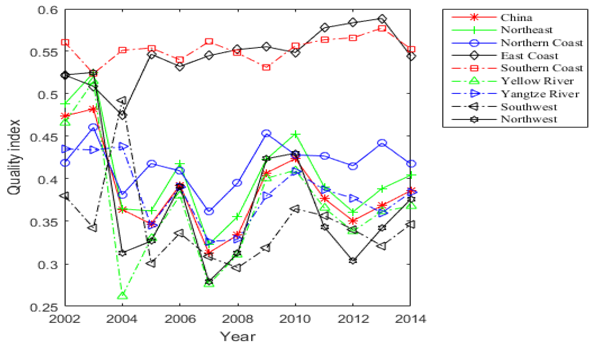
4.2.1. Trend of HSEE

The regional classification is defined by the Eight Regional Division Method, which was developed by China’s State Council Development Research Center. (The regional coordinated development strategy and policy report (2005) of China's State Council Development Research Center pointed out that the eastern, central, and western region partition method is inappropriate. Moreover, the report put forward that the mainland should be divided into eastern, central, west, and northeast as four big plate, and the four plates can be further divided into eight comprehensive economic zones, namely, northeast, northern coast, east coast, southern coastal, the middle reach of Yangtze River, the middle reaches of the Yellow River, southwest, and northwest regions.) Based on the results obtained from the previous stage, the quality index of HSEE was further estimated at the regional level by treating area ratio as the computing weight. Results are as shown in Figure 1, and the corresponding statistical descriptions of the indexes are shown in

Table 4. Statistical description of regional quality.

Region	Mean	Median	Standard Deviation	Min	Max
China	0.3861	0.3768	0.0505	0.3130	0.4822
Northeast	0.4043	0.3906	0.0570	0.3228	0.5247
Northern coast	0.4175	0.4180	0.0273	0.3613	0.4604
East coast	0.5446	0.5467	0.0311	0.4746	0.5887
Southern coast	0.5528	0.5540	0.0146	0.5238	0.5774
Yellow River	0.3680	0.3659	0.0704	0.2620	0.5149
Yangtze River	0.3842	0.3842	0.0379	0.3262	0.4378
Southwest	0.3465	0.3404	0.0506	0.2955	0.4927
Northwest	0.3760	0.3435	0.0798	0.2792	0.5252

.

According to Figure 1, the eastern and southern coasts are in the leading group, showing significantly higher average quality scores, above the national average, over the period 2002–2014. HSEE indexes of northeast, northern coast, Yellow River, Yangtze River, southwest, and northwest show similar trajectories in comparison to the overall trend of China. Year 2007 is a turning point. The indexes of all regions over the period 2002–2007 exhibit a fluctuating trend rather than a stable one. However, there is a sharp rise observed since 2009, and the variation tendency remains stable after 2010. On average, the HSEE index is 0.3861. Despite the obviously higher values observed in the eastern and southern coast regions, the average values of northeast, northern coast, Yangtze River, and northwest are close to the national average. However, the average annual indexes of the Yellow River and the southwest are only 0.3680 and 0.3465, respectively, which are both lower than the national average. Looking at the geographical distribution of quality index, there is an obvious aggregation. The division of the eight regions is not only the division of geographical location, but also the division of economic development level, indicating that the quality of HSEE in China is largely determined by geographic location and economic condition.

4.2.2. Difference of HSEE of Regions

Analyzing regional differences of HSEE and its sources can provide a realistic basis for policy-making.

Based on Formula (11), the differences in quality index of the eight regions are shown in

Table 5. Regional difference decomposition.

Region Year	Northeast	East Coast	Northern Coast	Southern Coast	Yellow River	Yangtze River	Southwest	Northwest	Intraregional Difference	Interregional Difference	Total
2002	3.4792	5.7077	3.8125	0.1000	4.8236	5.2389	6.1567	6.1607	35.4793	39.8119	75.2912
2003	3.6709	6.0726	3.7305	0.1000	5.1987	5.1562	5.3824	6.2997	35.6109	39.8669	75.4779
2004	2.8798	4.8725	3.5996	0.1000	3.8022	5.7807	9.6263	4.3223	34.9834	40.6713	75.6547
2005	3.2458	6.2033	4.8445	0.1000	4.7171	5.1286	6.0415	4.7029	34.9837	39.9072	74.8910
2006	3.4126	5.9609	4.3722	0.1000	4.8719	5.3263	6.3565	5.1213	35.5217	39.7818	75.3034
2007	3.0229	6.1693	5.1343	0.1000	4.2939	5.0844	6.6944	4.2294	34.7286	40.1437	74.8723
2008	3.2126	6.5317	5.0797	0.1000	4.4999	4.8990	6.0386	4.5302	34.8918	40.0523	74.9441
2009	3.4007	6.2632	4.3550	0.1000	5.0384	5.0715	5.8099	5.5577	35.5963	39.8235	75.4198
2010	3.4917	5.9872	4.1589	0.1000	4.9072	5.2000	6.4813	5.3350	35.6613	39.7744	75.4357
2011	3.2576	6.0649	4.6067	0.1000	4.8276	5.2531	6.6502	4.6236	35.3838	39.8776	75.2614
2012	3.1561	5.9873	4.8327	0.1000	4.7709	5.3899	6.6663	4.2226	35.1258	39.9812	75.1070
2013	3.3657	6.2713	4.7209	0.1000	4.9767	5.0023	5.8837	4.6347	34.9553	39.8772	74.8325
2014	3.3153	6.0184	4.4061	0.1000	4.7600	5.2266	6.5103	5.0305	35.3672	39.8176	75.1848
mean	3.3008	6.0085	4.4349	0.1000	4.7298	5.2121	6.4845	4.9824	35.2530	39.9528	75.2058

. We also estimated the contribution (in %) of each region to the overall regional difference, as shown in

Table 6. Regional difference contribution decomposition (unit: %).

Region Year	Northeast	East Coast	Northern Coast	Southern Coast	Yellow River	Yangtze River	Southwest	Northwest	Intraregional Difference	Interregional Difference
2002	4.6210	7.5809	5.0636	0.1328	6.4065	6.9582	8.1772	8.1826	47.1228	52.8772
2003	4.8635	8.0455	4.9424	0.1325	6.8877	6.8314	7.1311	8.3464	47.1806	52.8194
2004	3.8066	6.4405	4.7579	0.1322	5.0257	7.6408	12.7241	5.7131	46.2409	53.7591
2005	4.3340	8.2831	6.4688	0.1335	6.2986	6.8481	8.0671	6.2796	46.7129	53.2871
2006	4.5318	7.9158	5.8061	0.1328	6.4697	7.0731	8.4412	6.8009	47.1714	52.8286
2007	4.0374	8.2398	6.8574	0.1336	5.7349	6.7908	8.9410	5.6488	46.3838	53.6162
2008	4.2866	8.7154	6.7780	0.1334	6.0043	6.5369	8.0575	6.0448	46.5571	53.4429
2009	4.5090	8.3044	5.7744	0.1326	6.6804	6.7243	7.7034	7.3691	47.1976	52.8024
2010	4.6287	7.9368	5.5132	0.1326	6.5051	6.8933	8.5919	7.0722	47.2738	52.7262
2011	4.3283	8.0585	6.1209	0.1329	6.4145	6.9798	8.8362	6.1434	47.0145	52.9855
2012	4.2022	7.9717	6.4344	0.1331	6.3522	7.1762	8.8758	5.6221	46.7677	53.2323
2013	4.4977	8.3804	6.3087	0.1336	6.6504	6.6846	7.8625	6.1934	46.7114	53.2886
2014	4.4095	8.0048	5.8604	0.1330	6.3311	6.9516	8.6591	6.6908	47.0404	52.9596
mean	4.3890	7.9906	5.8989	0.1330	6.2893	6.9299	8.6206	6.6236	46.8750	53.1250

.

The mean difference in China’s HSEE index is 75.21 over the period 2002–2014, where interregional difference is 39.95 and its average annual contribution is 53.13%, and intraregional difference is 35.25 and its average annual contribution is 47.27%. The result implies that interregional and intraregional differences both are the main source of regional differences. Moreover, southwest shows the highest contribution level at 8.59%, followed by east coast, northwest, Yellow River, Yangtze River, north coast, and northeast. In contrast, southern coast’s contribution is limited at only 0.13%. A further longitudinal comparison found that the difference in the overall quality in China did not change dramatically over time.

5. Spatial Effect of HSEE

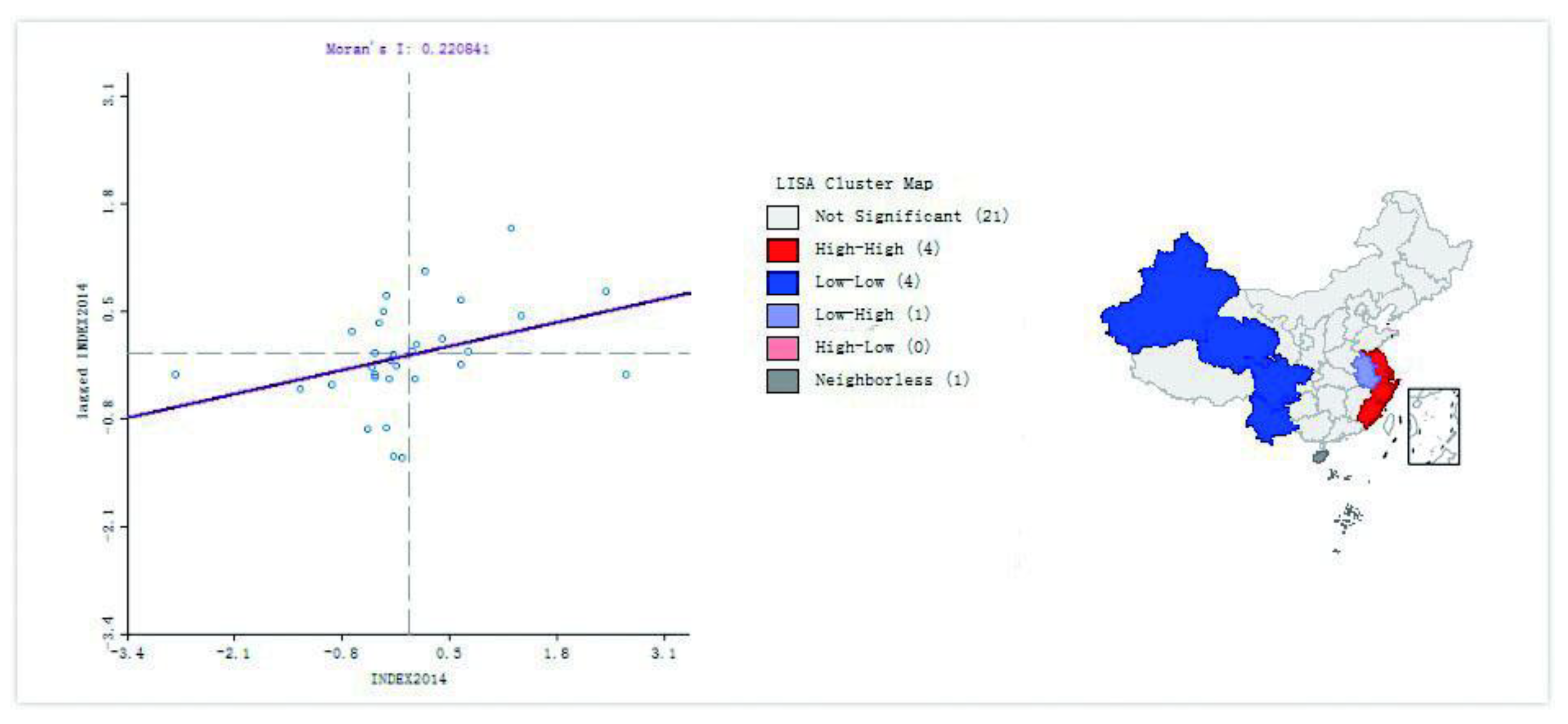
5.1. Spatial Correlation Analysis

Figure 2 shows a map in which each province is colored according to its mean value of human settlement ecological quality index over 2002–2014. It shows the distribution of HSEE quality across provinces. It is interesting to see that the ecological environmental quality index of human settlements in coastal areas is higher, but such a level of quality is gradually descending from the coast to inland. Furthermore, the corresponding Moran’s I index can be obtained by using the global autocorrelation model, as shown in

Table 7. Moran’s I from 2002 to 2014.

Year	2002	2003	2004	2005	2006	2007	2008
Moran’s I	0.1920 **	0.1024 *	0.2125 **	0.2908 ***	0.2713 ***	0.2039 ***	0.3078 ***
Year	2009	2010	2011	2012	2013	2014
Moran’s I	0.3134 ***	0.2148 **	0.1604 **	0.2601 ***	0.2701 ***	0.2208 **

***, **, * are significant at 1%, 5%, 10%, respectively.

. The figures in Table 7 describe the correlation degree and spatial agglomeration of the ecological environment quality index of HSEE in different regions of China during the sample period.

As shown in Table 7, the Moran’s I index is generally above 0.15 with significance. The only exception is year 2003. This result suggests that China’s HSEE quality has a strong positive spatial correlation. In other words, the areas with high/low quality index appear to be adjacent to areas with high/low quality index. For further researching the space agglomeration mode of regional quality, as an example, we produced a Moran scatter plot and LISA cluster diagram for 2014, as shown in Figure 3. The first, the second, the third, and the fourth quadrant of the Moran scatter plot correspond to High–High, Low–High, Low–Low, High–Low, respectively. The corresponding Moran’s I index in the first and the third quadrants are positive, indicating a positive spatial correlation, while the corresponding Moran’s I index in the third and the fourth quadrants are negative, indicating that there is a negative spatial correlation in quality indexes. As can be seen from the Figure 3, most points fall into the first quadrant and the third quadrant, while only a few points fall into the second and the fourth quadrant. Specifically, Jiangsu, Shanghai, Zhejiang, and Fujian fall into High–High region, and Xinjiang, Qinghai, Sichuan, and Yunnan fall into Low–Low region. During the study period, the global spatial autocorrelation index and local autocorrelation are both significant, indicating that there is spatial clustering and difference in the quality of China’s human settlement ecological environment.

5.2. Selection and Estimation of Spatial Panel Model

This study chose the factors that influence the quality of HSEE, such as foreign trade, environmental control, economic development level, energy structure, energy intensity, urbanization level, and residents’ quality (as shown in 3.4) for seeking the possible implementation path for improving human settlement ecological quality.

In order to estimate the coefficients of the abovementioned factors correctly, it is necessary to select the most suitable parameter estimation in basic spatial panel models (namely, Formulas (12)–(14)). We first estimated the model that does not contain spatial interaction and calculated the corresponding Lagrange Multiplier (LM) statistic, the joint significance test of spatial fixation effect, and the time fixation effect, as shown in

Table 8. Nonspatial panel model estimation and LM test.

Variable	Mixed Estimation	Spatial Fixation	Time Fixation	Spatial and Time Fixation
C	0.0514 **	-	-	-
	(−2.2680)
exp	0.2983 ***	−0.1040 *	0.2252 ***	−0.1156 *
	(10.3594)	(−1.6973)	(7.8568)	(−1.9078)
er	−0.0278	0.0192	−0.0002	0.0605
	(−0.5481)	(0.3630)	(−0.0048)	(1.2108)
ec	0.0358	−0.3199	−0.1015	−0.6356
	(0.0775)	(−0.6751)	(−0.2464)	(−1.4322)
city	−0.0852	0.0515	0.0879	0.0667
	(−1.3719)	(0.5330)	(1.4946)	(0.7443)
lpgdp	0.0139	−0.0565	0.0324 ***	−0.0038
	(1.5826)	(−1.4334)	(3.9756)	(−0.0832)
edu	0.0187 **	0.0209	−0.0094	−0.0066
	(2.1225)	(1.4667)	(−1.0855)	(−0.3724)
en	0.0008	−0.0113 **	−0.0025	−0.0091
	(0.4283)	(−2.0554)	(−1.5471)	(−1.6482)
R2	0.5786	0.1081	0.6497	0.7929
LogL	431.1768	537.8759	481.6372	574.2983
LM spatial lag	37.5064	39.8704	8.6459	5.2345
	0.0000	0.0000	0.0030	0.0220
LM spatial error	40.3117	36.2078	7.3378	4.8821
	0.0000	0.0000	0.0070	0.0340
Robust LM spatial lag	3.0000	4.8235	1.8279	5.8279
	0.0830	0.0280	0.1760	0.0160
Robust LM Spatial error	5.8053	1.1610	0.5897	4.8821
	0.0160	0.2810	0.4430	0.0340
spatial fixation LR test	185.3223 (0.0000)
time fixation LR test	72.8448 (0.0000)

***, **, * are significant at 1%, 5%, 10%, respectively, the corresponding t statistic shown in brackets.

.

According to the results of the joint effect test, the spatial and temporal effects are rejected at the significance level of 1%, indicating that the model should be fixed in space and time. Therefore, LM statistics should be on the basis of a double fixed model. It can be seen from Table 8 that the LM statistic rejects the null hypothesis at a significance level of 5%, indicating that the SAR and SEM models exist simultaneously. Therefore, it is necessary to use the SDM model to estimate the coefficients, namely, Formula (14). The coefficients of the SDM model can be estimated using Matlab, as shown in

Table 9. Estimation results of spatial Durbin model.

Variable	Coefficient	Variable	Coefficient
W*SQI	0.1610 **
	(2.4548)
exp	−0.1185 *	W*exp	0.3504 ***
	(−1.8740)		(3.2212)
er	0.0764	W*er	0.2741 **
	(1.5678)		(2.2112
ec	−0.7559 *	W*ec	−2.6314 **
	(−1.7422)		(2.2998)
city	0.0842	W*city	0.2168
	(0.9703)		(1.0418)
lpgdp	−0.0182	W*lpgdp	0.0222
	(−0.3935)		(0.2159)
edu	−0.0159	W*edu	−0.0531
	(−0.8802)		(−1.2623)
en	−0.0035	W*en	0.0332 **
	(−0.5657)		(2.1316)
R2	0.8079	Log L	588.2614
Wald test spatial lag	24.2933	Wald test spatial error	23.0472
	0.0020		0.0033

(***, **, * are significant at 1%, 5%, 10%, respectively, the corresponding t statistic shown in brackets).

.

From the results of two Wald statistic tests, we can see that the SDM model cannot be simplified as the SAR model or the SEM model. It is appropriate to apply the SDM model, a broader form, for analysis. The coefficient of the spatial lagged explanatory variable $W\times SQI$ is 0.1610 and it is significant at 5%, indicating that there is a spatial spillover effect on quality of HSEE. The improvement of the quality in one province could have a positive effect on the improvement in its neighboring provinces. According to the spatial lag variables and the significance of the equation, the spatial effect of factors should be included in the analysis.

5.3. Direct Effect and Indirect Effect Analysis

According to the estimation results in Table 9 and together with the Formulas (19) and (20), the direct effect, indirect effect, and total effect of the explanatory variables on HSEE quality can be obtained. The results are shown in

Table 10. Effect of variables on ecological environment.

Variable	Direct Effect	Indirect Effect	Total Effect
exp	−0.1043	0.3815 ***	0.2771 *
	(−1.5905)	(2.8671)	(1.7882)
er	0.0899 *	0.3324 **	0.4224 **
	(1.7952	(2.3591)	(2.5925)
ec	−0.8854 *	−3.1950 **	−4.0803 ***
	(−1.9948)	(−2.4687)	(−2.7526)
city	0.0948	0.0228	0.3647
	(1.1080)	(0.1913)	(1.3360)
lpgdp	−0.0204	0.0355	0.0024
	(−0.4615)	(0.4014)	(0.0185)
edu	0.0179	0.0646	0.0825
	(0.9286)	(1.2869)	(1.3470)
en	0.0021 *	0.0374 *	0.0395 **
	(0.3264)	(2.0011)	(4.7200)

***, **, * are significant at 1%, 5%, 10%, respectively, the corresponding t statistic shown in brackets.

.

From Table 10, the direct effect of export trade is negative, but it is not significant. This indicates that excessive reliance on exports would compromise the quality of human settlements to a certain extent. According to Zhu [41], China’s export trade scale is the cause of changes in industrial pollutant emissions, and the scale of export trade and industrial emissions are positively correlated. Thus, the rapid expansion of China’s export trade causes a certain negative impact on the environment. However, the expansion of export trade would increase resource consumption, and it contributes to economic growth, which makes the direct effect insignificantly negative. The indirect effect is 0.3815, and it is significant at the 1% level, showing that export trade has a positive spillover effect on the improvement of ecological environment. This is likely caused by the existence of the “export squeeze effect”. The province’s exports could promote its neighboring provinces to upgrade industrial structure and stimulate technological innovation, which further improves technological complexity of export products, reduces energy consumption, and eventually encourages neighboring provinces to achieve a win-win in the situation between export and ecological environment protection.

The direct effect of environmental control is significantly positive at a 10% confidence level. This fact indicates that policy interventions—such as strengthening environmental control, improving production technology standards, and increasing the limits of sewage restrictions—is likely to significantly enhance the quality of the human settlement ecological environment at the provincial level. The indirect effect is also significant, indicating that the environmental control has a positive spillover effect. Strengthening environmental control will not only improve the quality of the human settlement ecological environment in the province itself, but also will improve the ecological environment in its neighborhood. The effect is beneficial for China to improve ecological environments, which is consistent with previous assertions (e.g., Mao et al. [42]).

The direct effect and indirect effect of energy structure are significantly negative, which shows that reducing dependence on coal consumption and improving the energy consumption structure can not only improves the quality of HSEE in the province itself, but also can significantly improve the HSEE quality of neighboring provinces. The reason may be that coal combustion would produce a lot of sulfur dioxide, nitrogen oxides, and soot, and these pollution emissions not only cover the province itself but can also spread with the flow of atmosphere, which increases the concentration of pollutants in neighboring provinces.

The direct effects of urbanization, economic development level, and residents’ quality on improvement of ecological environment quality are not significant, and their indirect effects are also not significant. The results may be in relation to the agglomeration effect. The effects are no longer significant with the expansion of geographical distance.

The direct effect of energy intensity is significantly positive at 0.0021, which indicates that improvement of energy intensity can significantly improve the HSEE quality. The indirect effect is also significant, showing a positive spillover effect of energy intensity. This is because energy intensity improvement mainly depends on technological progress, which has a spatial spillover effect [43]. The positive externality from technological progress in one province can be delivered to neighboring provinces, and accordingly promote the improvement of energy intensity there.

6. Conclusions and Discussion

This paper constructed an index system from a perspective of strong sustainability and measured China’s human settlement ecological environment (HSEE) quality through the projection pursuit method. The analysis of its regional differences and spatial effects were also included.

The HSEE quality in China was declining in general; over the period 2002–2014, it decreased from 0.4740 to 0.3861. Therefore, the environmental pressure was still prominent in many of the regions in China. The following regional analysis reveals that the HSEE quality of the eastern coast and southern coast was comparatively in fine condition, with average index values of 0.5446 and 0.5528, respectively. The average quality index of northeastern and northern coast are both close to 0.4, and their quality scores were higher than the national average. The quality index of the Yangtze River and northwest were close to the national level. On the contrary, the quality index of Yellow River and southwest region were lower than the national level. At the provincial level, findings show that the quality of HSEE would be affected by geographical locations.

There were differences with low time variant variations in HSEE quality across provinces in China. However, the intraregional and interregional differences could not be overlooked, and their contributions to total difference are both close to 50%. Areas with lower HSEE quality contributed more to total differences. Therefore, ecological policy formulation and implementation should take into account such differences, both generally and spatially.

A spatial spillover effect of HSEE quality across China’s provinces was identified. The improvement of quality in single province could have a positive effect on the quality improvement in its neighboring provinces. Among influence factors of HSEE quality, the direct effect of foreign trade was negative, but its indirect effect was significantly positive. The direct effect and indirect effect of environmental regulation, energy structure, and energy intensity were significantly positive. The effect of urbanization, economic development level, and residents’ quality were not significant.

Faced with the less optimistic fluctuation of HSEE, China should intensify efforts to control and improve the ecological quality. Improving ecological quality of Yangtze River, southwest, northwest, and Yellow River is crucial for Chinese government in setting up HSEE. Due to the geographical location, agglomeration of HSEE and regional differences should not be neglected. Achieving the coordinated development of HSEE is not to avoid its spatial accumulation. On the contrary, it should adjust the supporting facilities, policies, and economic development patterns in regions with lower HSEE quality and make full use of spillover effect from regions with that of high quality to promote the coordinated development across areas. Overall, improving environmental control, adjusting the energy structure, and improving the energy intensity are the feasible ways for China to improve HSEE quality.

The research, from the perspective of strengthening HSEE, also proved the validation of the integrative development framework. In comparison to past research, which only focused on testing the impact of single/multiple factors on environment quality, this paper introduced the concept of sustainability, and further incorporated it into the existing theoretical framework.

This paper makes two empirical contributions. On one hand, the coordinating development of HSEE relies on the availability of the spillover effect of environmental control, energy structure, and energy intensity. On the other hand, policy measures at the aggregate level may result in biases as significant heterogeneity and spatial effects present among provinces. This implies that a one-size-fits-all solution may be inappropriate for improving HSEE quality at the regional level. Each province may develop its own policy measures and consider how to aid/mitigate positive/negative influence from its neighborhoods.

References

1. Study on Desertification Control in China. Study on the Control of Desertification (Land Degradation) in China; China Environmental Science Press: Beijing, China, 1998. [Google Scholar]
2. National Bureau of Statistics of China. China Statistical Yearbook; China Statistics Press: Beijing, China, 2016.
3. Yang, W.P.; Zhao, J.K. Sources of China’s economic growth: A Case for green accounting. Adv. Manag. Appl. Econ. 2018, 8, 33–59. [Google Scholar]
4. Liu, Q.P.; Lin, Z.S.; Feng, N.H. Evaluation on the spatial differences of urban settlement environment of Jiangsu province. Areal Res. Dev. 2005, 24, 30–33. [Google Scholar]
5. Zhao, Y.D.; Zhang, H.; Chen, X.P. Evaluation of city inhabitable environment quality by objective index system. J. Arid Land Resour. Environ. 2009, 4, 1–5. [Google Scholar]
6. Zhang, W.X.; Wang, R. Analyses on the current situation of urban human settlement environment in China. Urban Stud. 2007, 2, 115–120. [Google Scholar]
7. Sun, Y.; Cheng, Q.G.; Li, Y.; Fu, J. Assessment of eco-economic system sustainable development of Liaoning province based on energy analysis. Chin. J. Appl. Ecol. 2014, 25, 188–194. [Google Scholar]
8. Gao, J.X. Study on the Theory of Sustainable Development; China Environmental Science Press: Beijing, China, 2001. [Google Scholar]
9. Wang, K.Y. Compound Model System of Ecological Carrying Capacity and Its Application; Science Press: Beijing, China, 2007. [Google Scholar]
10. Geddes, P. Cities in Evolution: An Introduction to the Town Planning Movement and the Study of Civicism; Howard Ferug: New York, NY, USA, 1915. [Google Scholar]
11. Howard, E. Garden Cities of Tomorrow; Faber and Faber: London, UK, 1946. [Google Scholar]
12. Mumfond, L. The City in History: Its Origin, Its Transformation, and Its Prospects; Harcourt, Brace & World, Inc.: New York, NY, USA, 1961. [Google Scholar]
13. Doxiadis, C.A. Ekistics: An Introduction to the Science of Human Settlements; Athens Publishing Center: Athens, Greece, 1968. [Google Scholar]
14. Arnfield, A.J. Two decades of urban climate research: A review of turbulence, exchanges of energy and water, and the urban heat island. Int. J. Climatol. 2003, 23, 1–26. [Google Scholar] [CrossRef]
15. Jenerette, G.D.; Harlan, S.L.; Brazel, A.; Jones, N.; Larsen, L.; Stefanov, W.L. Regional relationships between surface temperature, vegetation, and human settlement in a rapidly urbanizing ecosystem. Landsc. Ecol. 2007, 22, 353–365. [Google Scholar] [CrossRef]
16. Walter, J. Ecological role of lactobacilli in the gastrointestinal tract: Implications for fundamental and biomedical research. Appl. Environ. Microbiol. 2008, 74, 4985. [Google Scholar] [CrossRef] [PubMed]
17. McGranahan, G.; Balk, D.; Anderson, B. The rising tide: Assessing the risks of climate change and human settlements in low elevation coastal zones. Environ. Urban. 2007, 19, 17–37. [Google Scholar] [CrossRef]
18. Talen, E. Neighborhood-level social diversity: Insights from Chicago. J. Am. Plan. Assoc. 2006, 72, 431–446. [Google Scholar] [CrossRef]
19. Clos, J. Keynote speech in International Symposium on Sciences of Human Settlements. In Proceedings of the International Symposium on Sciences of Human Settlements, Beijing, China, 25–28 June 2011. [Google Scholar]
20. Zhao, L.; Lin, Z.; Ma, H.Q. Analysis on temporal and spatial variation about living environment of the cities on Northeastregion. Areal Res. Dev. 2013, 2, 73–78. [Google Scholar]
21. Sui, Y.Z.; Shi, J. Integrated assessment of ecological quality for human settlements in Shanghai. Resour. Environ. Yangtze Basin 2013, 8, 965–971. [Google Scholar]
22. Yang, Y.Z.; Guo, G.M. Natural environment suitability for human settlements in Inner Mongolia based on GIS. J. Arid Land Resour. Environ. 2012, 3, 9–16. [Google Scholar]
23. Li, J.C.; Wang, W.L.; Hu, G.Y.; Wei, Z. Impacts of land use and land cover change on ecosystem service values in Maqu County. China Environ. Sci. 2010, 11, 1579–1584. [Google Scholar]
24. Liu, X.; Feng, Q. Evaluation of ecological services value of alpine rangeland ecosystem in the northern Tibet region. Acta Sci. Circumst. 2012, 12, 3152–3160. [Google Scholar]
25. Li, D.; Ren, Z.; Liu, X.; Lin, Z. Dynamic change of ecological service value of cultivated land in Shaanxi Province. J. Arid Land Resour. Environ. 2013, 7, 40–45. [Google Scholar]
26. Feng, Z.M.; Tang, Y.; Yang, Y.Z.; Dan, Z. The relief degree of land surface in China and its correlation with population distribution. J. Geogr. Sci. 2007, 10, 1073–1082. [Google Scholar]
27. Yang, J.; Yang, X.M.; Li, Y.H.; Sun, C.Z.; Wang, F.X. Assessment on spatial differences of human settlement environment in communities cased on DPSIRM model: The case study of Dalian. Geogr. Res. 2012, 1, 135–143. [Google Scholar]
28. Li, X.M.; Jin, P.Y. Characteristics and spatial-temporal differences of urban human settlement environment in China. Sci. Geogr. Sin. 2012, 5, 521–529. [Google Scholar]
29. Xu, W.; Zhang, G.; Li, X.; Zou, S.; Li, P.; Hu, Z.; Li, J. Occurrence and elimination of antibiotics at four sewage treatment plants in the Pearl River Delta (PRD), South China. Water Res. 2007, 19, 4526–4534. [Google Scholar] [CrossRef] [PubMed]
30. Li, Q. Effects of urbanization on summer extreme warmest night temperature changes in surrounding Bohai Area. Sympos. Urban Environ. 2013, 15, 23–45. [Google Scholar]
31. Zhao, H.; Che, H.; Zhang, X.; Ma, Y.; Wang, Y.; Wang, H.; Wang, Y. Characteristics of visibility and particulate matter (PM) in an urban area of Northeast China. Atmos. Pollut. Res. 2013, 4, 427–434. [Google Scholar] [CrossRef]
32. Li, J.; Li, X.M.; Liu, Z.Q. Assessment and analysis on urban human settlement ecology environment based on degree of urbanization development: Case study of Dalian, Liaoning province. China Popul. Resour. Environ. 2009, 1, 156–161. [Google Scholar]
33. Pearce, D.W. Blueprint: For a Green Economy; Earthscan Ltd.: London, UK, 1989. [Google Scholar]
34. Fujii, S.; Cha, H.; Kagi, N.; Miyamura, H.; Kim, Y. Effects on air pollutant removal by plant absorption and adsorption. Build. Environ. 2005, 1, 105–112. [Google Scholar] [CrossRef]
35. Roca, J.; Serrano, M. Income growth and atmospheric pollution in Spain: An input–output approach. Ecol. Econ. 2007, 1, 230–242. [Google Scholar] [CrossRef]
36. Gawande, K.; Bohara, A.K.; Berrens, R.P.; Wang, P. Internal migration and the environmental Kuznets curve for US hazardous waste sites. Ecol. Econ. 2000, 1, 151–166. [Google Scholar] [CrossRef]
37. Hao, Y.; Liu, Y.M. The influential factors of urban PM 2.5 concentrations in China: A spatial econometric analysis. J. Clean. Prod. 2016, 112, 1443–1453. [Google Scholar] [CrossRef]
38. National Environmental Protection Bureau. Technical Criterion for Ecosystem Status Evaluation; National Environmental Protection Bureau: Beijing, China, 2015.
39. Caussinus, H.; Ruiz-Gazen, A. Exploratory Projection Pursuit: Data Analysis; ISTE: Washington, DC, USA, 2016; pp. 249–266. [Google Scholar]
40. Pace, R.K.; Lesage, J.; Zhu, S. Impact of cliff and ord on the housing and real estate literature. Geogr. Anal. 2009, 4, 418–424. [Google Scholar] [CrossRef]
41. Zhu, Q. Empirical analysis on the relationship between export and industrial pollution & controlling in China. World Econ. Study 2007, 8, 47–51. [Google Scholar]
42. Mao, M.; Deng, Y.; Sun, J. Research on China’s regional carbon emission and environment regulation spillovers. Sci. Technol. Manag. Res. 2016, 7, 235–239. [Google Scholar]
43. Zhang, C.J.; Zhang, Z.Y. The spatial effect of energy endowment and technological progress on China’s carbon emission intensity. China’s Popul. Resour. Environ. 2015, 9, 37–43. [Google Scholar]
Figure 1. Change curves of regional HSEE quality.
Sustainability 10 01520 g001
Figure 2. Average distribution of China’s regional ecological environmental quality index.
Sustainability 10 01520 g002
Figure 3. The concentration of ecological environment quality index in China in 2004.
Sustainability 10 01520 g003