Economic and Environmental Evaluation of a Brick Delivery System Based on Multi-Trip Vehicle Loader Routing Problem for Small Construction Sites

Abstract

While large construction sites have on-site loaders to handle heavy and large packages of bricks, small brick manufacturers employ a truck-mounted loader or sometimes deploy a loader truck to accompany normal brick delivery trucks to small construction sites lacking on-site loaders. It may be very challenging for small contractors to manage a sustainable delivery system that is both cost-effective and environmentally friendly. To address this issue, this paper proposes to solve a multi-trip vehicle loader routing problem by uniquely planning routes and schedules of several types of vehicles considering their synchronized operations at customer sites and multi trips. This paper also evaluates the sustainability of the developed model from both economic and environmental perspectives. Case studies based on small construction sites in the Middle East demonstrate applications of the proposed model to make the most economical plans for delivering bricks. Compared to the single-trip vehicle loader routing problem, the proposed model reduces, on average, 18.7% of the total delivery cost while increasing CO₂ emission negligibly. The economic benefit is mainly achieved by reducing the required number of vehicles. Brick plant managers can use the proposed mathematical model to plan the most cost-effective delivery schedules sustainably while minimizing negative environmental effects.

1. Introduction

Most large brick manufacturers deliver bricks to construction sites where on-site equipment (e.g., crane and forklift) unloads heavy packages of bricks from trucks. On the other hand, small manufacturers deliver bricks generally to small construction sites where on-site unloader(s) are usually not available. Thus, to unload heavy and large packages of bricks, they need to deliver bricks using a loader-mounted truck (called a loader truck) or sometimes a normal truck accompanied by a loader truck. Since a loader truck can operate independently, it is possible to schedule its operations so that it can visit the construction sites briefly to assist unloading of other normal trucks where loader(s) are not in presence.

This paper addresses a scheduling and routing problem to dispatch two types of trucks (i.e., loader and normal trucks) for delivering bricks to small construction sites where on-site loaders are mostly unavailable. Specifically, it considers multi trips as well as synchronized operations of two types of trucks to unload large and heavy packages of bricks at customer sites.

For transporting heavy or large products, several industrial fields (e.g., the shipping and the dairy industries) employ logistics systems with several types of vehicles. Chao (2002) [1] addresses a truck and trailer routing problem while Derigs et al., (2013) [2] develop heuristics to solve it more effectively. Drexl (2012) [3] describes a generalized concept of operation synchronization for load transfers at transshipment locations based on examples in the dairy industry. Chen et al., (2013) [4] develop a model for a truck scheduling problem considering crane handling in a maritime container terminal. In 2016, An and Byon [5] introduced the single-trip vehicle loader routing problem (VLRP), which is a new extended model from the typical vehicle routing problem (VRP). It plans routing schedules of several types of vehicles such as a loader and a normal truck for delivering products from a depot to customers. The VLRP incorporates time windows at customer sites as a deciding factor. To the best of our knowledge, such concept of imposing time windows at customer sites as deciding variables in VRP has been addressed in 2015 [6] for the first time.

Since the VRP was introduced by Dantzig and Ramser in 1959 [7], many researchers have studied variants of the VRP, for example, VRP with time windows [8], multi-depot VRP [9], VRP with backhauls [10], heterogeneous VRP [11], multi-trip VRP (MTVRP) [12].

The concept of multi trips in routing problems has been addressed in 1987 [13] considering up to double trips. In 1994 [12], the first complete MTVRP model was formulated using a real-world distribution system. Since [12], the MTVRP has been studied by many researchers mainly for overcoming its computational difficulties. In efforts to find a good solution of the MTVRP in a relatively short time, Brandão and Mercer (1998) [14] developed an algorithm based on the Tabu search. Several exact solution methods for finding an optimal solution of the MTVRP also have been developed: a branch-and-cut algorithm [15], column-and-cut generation algorithm [16], and a two-phase exact algorithm [17]. In addition to solution methods, Zhang et al., (2015) [18] incorporated replenishment operations into the MTVRP, and Cattaruzza et al., (2016) [19] considered release dates additionally in the MTVRP. A few survey papers for routing problems [15,20] entails further details on the past studies.

Recently, a few studies considered environmental aspects in product delivery problems such as urban freight truck routing [21], sustainable e-commerce delivery [22], production and green transportation [23].

Even though there are many variants of the VRP in the literature, studies in the past have not addressed VRP with collaborative operations at customer sites and multi trips simultaneously. Thus, this paper presents a multi-trip vehicle loader routing problem (MTVLRP) which entails scheduling of several types of vehicles considering their synchronized unloading operations at customer sites as well as multi-trips. Also, since synchronized operations with a loader and a normal truck are generally required in small construction sites due to unavailability of on-site loaders, small brick manufacturers should deal with more complicated route scheduling than large manufacturers. In addition, freight trucks are one of the major sources of greenhouse gas emissions in metropolitan areas [21]. Small brick manufacturers also may be interested in reducing greenhouse gas emissions to promote their reputation as a marketing strategy by acting in accordance with the efforts of the government to reduce greenhouse gas emissions and to prepare proactively for carbon emissions trading in the future. Therefore, planning a sustainable brick delivery system that is economical and yet environmentally friendly (e.g., CO₂ emission reduction) can be very challenging especially for small manufacturers.

As such, it would be motivating and essential to check if we can achieve both economic viability and environmentally friendliness in the brick delivery system applicable to different sizes of brick manufacturers. In addition, another related interesting question to address is how cost effective can brick delivery system be that is environmentally friendly.

However, to our best knowledge, no study has addressed this issue, and therefore no practical solutions exist. Thus, the objectives of this paper are (1) to develop the most cost-effective brick delivery system to small construction sites and (2) to evaluate the sustainability of the developed system in both economic and environmental perspectives.

The rest of the paper is comprised as follows. Section 2 describes the problem statement and presents mathematical models of both the VLRP and the MTVLRP. Section 3 provides a case study using close real-world problems in the brick industry and shows experiment results and analysis. Section 4 discusses the usefulness of MTVLRP in both economic and environmental perspectives. Finally, Section 5 concludes the paper.

2. Materials and Methods

This section describes the problem statement and presents the mathematical modeling.

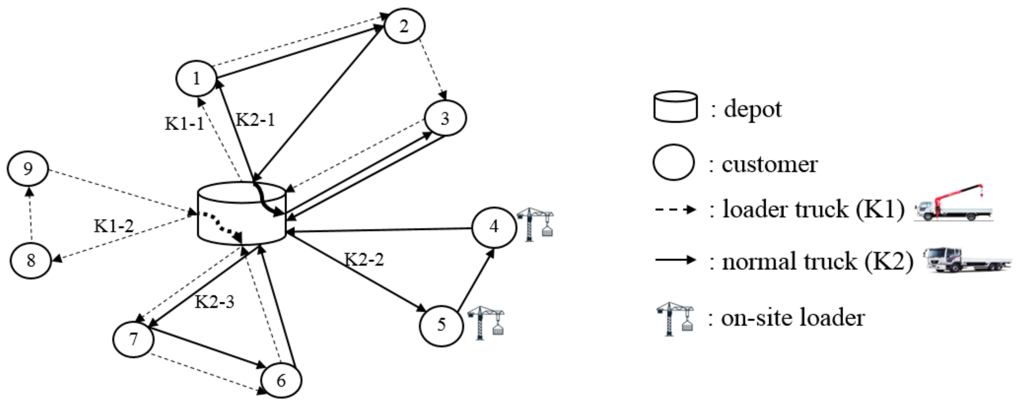
2.1. Problem Statement

The overall system of the MTVLRP is similar to that of the VLRP [5] except that each vehicle can travel multiple times. The network of VLRP, from a context of a delivery system of heavy or large products from a depot to several customers, is comprised of one depot and several satellite locations, each of which corresponds to each customer. Trucks deliver products to customers from the depot and need to return during working hours, generally within a day. Unloading heavy or large products at a customer site requires a loader when a normal truck arrives at the site. If a customer site has an on-site loader, then, a normal truck can deliver products to the site freely. Otherwise, at least one moving loader (i.e., a loader truck) needs to visit the site. For the latter case, a normal truck can visit the customer site together with a loader truck to deliver larger amounts of the products. It is noted that in this case, it is also possible that the loader truck can accompany another normal truck when visiting a small construction site, and stay there only for the duration of unloading the normal truck and continue on with its independent schedule ahead. In other words, the loader truck can also be treated as a mobile loader equipment.

In addition to the requirements of the VLRP described above, the MTVLRP allows a vehicle to return to the depot and depart again to deliver products to other customers. For constructing the problem, a few following assumptions are employed. First, two types of vehicles are used: loader and normal trucks. Second, all vehicles need to depart from the depot and return to it before the end of a planning time horizon (i.e., working hours). Third, all vehicles returned to the depot can depart again. Fourth, each vehicle can visit a customer site up to once in order to avoid sub-tours. Fifth, a customer’s demand at each node can be greater than the capacity of a truck so that several vehicles can deliver products to the same customer site to meet the demand. Lastly, the traveling speed of one vehicle type can be different to that of other vehicle types. This will add flexibility to the proposed model which will be able to handle different vehicle performances or real-time traffic conditions associated with road congestions, in the future.

Figure 1 depicts a typical example of the MTVLRP, which is comprised of one depot and nine customer sites. Loader trucks need to visit all customer sites except two sites which hold an on-site loader (i.e., nodes 4 and 5). K1 and K2 represent a loader truck and a normal truck, respectively: two loader trucks and three normal trucks are employed (i.e., K1-1, 2, and K2-1, 2, 3).

Both types of vehicles visit together each customer sites (i.e., nodes 1, 2, 3, 6 and 7) in the same time window for synchronized unloading operations: i.e., loader truck K1-1 and normal truck K2-1 visit nodes 1, 2 and 3; and loader truck K1-2 and normal truck K2-3 visit nodes 6 and 7. Also, the example shows that loader truck K1-1 and normal truck K2-2 depart the depot again after returning to it, making additional routes and reducing the required number of vehicles compared to the VLRP.

2.2. Mathematical Modeling

This section provides a mathematical model of the MTVLRP which determines the number of vehicles of each type, their potential collaborations considering multiple trips, beginning and ending times of unloading products at customers’ sites, and amounts of products delivered to each customer by each vehicle.

Table 1. Notations for the multi-trip vehicle loader routing problem (MTVLRP).

Indices

i, j: node indices

k: vehicle type

n: vehicle index

Set

$E_i^{-}\left(E_i^{+}\right)$: set of arcs incident from (to) a node i

E: set of arcs

K: set of vehicle types ($k$ = 1: loader truck, $k$ = 2: normal truck)

$N^k$: set of vehicles of a vehicle type $k$ ($k\in K$)

$V_1$: set of nodes where a loader is needed

$V_2$: set of nodes where a loader is not needed (i.e., an installed loader exists)

$V_r$: set of nodes from which arcs are incident to a depot ($V_r=\left\{i:\left(i,0\right) \in E_0^{+}\right\}$)

$V_s$: set of nodes to which arcs are incident from a depot ($V_s=\left\{j:\left(0,j\right) \in E_0^{-}\right\}$)

V: set of nodes except a depot ($V=V_1{{\displaystyle \cup }}^{\text{}}{V}_2$)

$\widehat{V}$: set of all nodes ($\widehat{V}=\left\{0\right\}{\displaystyle \cup }{V}_1{\displaystyle \cup }{V}_2$)

Parameters

$C{T}^k$: transportation cost per unit time by a vehicle type k

$C{W}^k$: waiting cost per unit time by a vehicle type k

$D_i$: demand at node i.

M: big number

$P^k$: vehicle cost of a vehicle type k during a planning horizon

$Q^k$: capacity of a vehicle type k

$T{R}_{ij}^k$: travel time between nodes i and j by a vehicle type k

$TL$: average time to load (unload) product at a depot (at customers’ sites)

$TM$: length of the planning horizon

defines all notations used. Several sets of nodes related to a depot (i.e., $V_r,V_s$ and $\widehat{V}$) use a node index of ‘0’ to represent the depot.

Since the MTVLRP extends the VLRP and incorporates vehicle costs into the objective function by using slightly different notations compared to the prior VLRP formulation provided by An and Byon (2016), the formulation of the VLRP is presented here first. To prescribe appropriate schedules of vehicle routes and unloading operations, the VLRP incorporates one type of binary decision variables:

• $x_{ijkn}$: 1 if an arc (i, j) is used by a nth vehicle of a type k, 0 otherwise, and five types of continuous decision variables,
• $a_{ikn},b_{ikn}$: beginning and ending times of an unloading operation by a nth vehicle of a type k, at a node i,
• $s_{jkn},r_{ikn}$: departing time from a depot to node j and returning time from node i to a depot of a nth vehicle of a type k,
• $z_{ikn}$: amounts of products delivered to node i by a nth vehicle of a type k.

By using all notations in Table 1 and aforementioned decision variables, here we present a mixed integer linear programming model for the VLRP as follows.

$$\mathrm{VLRP}:min{{\displaystyle \sum }}_{\left(i,j\right)\in E}{{\displaystyle \sum }}_{k\in K}{{\displaystyle \sum }}_{n\in N^k}C{T}^{k}T{R}_{ij}^k{x}_{ijkn}+{{\displaystyle \sum }}_{i\in V}{{\displaystyle \sum }}_{k\in K}{{\displaystyle \sum }}_{n\in N^k}C{W}^K\left(b_{ikn}-a_{ikn}\right)$$

(1)

s.t.

$$\begin{array}{lll}{{\displaystyle \sum }}_{k\in K}{{\displaystyle \sum }}_{n\in N^k}{z}_{ikn}\ge D_i,& & i\in V\end{array}$$

(2)

$$\begin{array}{lll}{{\displaystyle \sum }}_{\left(j,i\right)\in E_i^{+}}{x}_{jikn}\le 1,& & i\in V,k\in K,n\in N^k\end{array}$$

(3a)

$$\begin{array}{lll}{{\displaystyle \sum }}_{\left(j,i\right)\in E_i^{+}}{x}_{jikn}-{{\displaystyle \sum }}_{\left(i,j\right)\in E_i^{-}}{x}_{ijkn}=0,& & i\in \widehat{V},k\in K,n\in N^k\end{array}$$

(3b)

$$\begin{array}{lll}{b}_{ikn}-a_{ikn}-TL{{\displaystyle \sum }}_{\left(j,i\right)\in E_i^{+}}{x}_{jikn}\ge 0,& & i\in V,k\in K,n\in N^k\end{array}$$

(4)

$$\begin{array}{lll}{a}_{i{k}_1{n}_1}-a_{i{k}_2{n}_2}-M\left(2-{{\displaystyle \sum }}_{\left(j,i\right)\in E_i^{+}}{x}_{ji{k}_1{n}_1}-{{\displaystyle \sum }}_{\left(j,i\right)\in E_i^{+}}{x}_{ji{k}_2{n}_2}\right)\le 0,& & i\in V_1,k_1\in K_1,n_1\in N^{k_1},k_2\in K{K}_1,n_2\in N^{k_2}\end{array}$$

(5a)

$$\begin{array}{lll}{b}_{i{k}_1{n}_1}-b_{i{k}_2{n}_2}+M\left(2-{{\displaystyle \sum }}_{\left(j,i\right)\in E_i^{+}}{x}_{ji{k}_1{n}_1}-{{\displaystyle \sum }}_{\left(j,i\right)\in E_i^{+}}{x}_{ji{k}_2{n}_2}\right)\ge 0,& & i\in V_1,k_1\in K_1,n_1\in N^{k_1},k_2\in K{K}_1,n_2\in N^{k_2}\end{array}$$

(5b)

$$\begin{array}{lll}{r}_{ikn}\le TM,& & i\in V_r,k\in K,n\in N^k\end{array}$$

(6)

$$\begin{array}{lll}{a}_{jkn}-b_{ikn}+M\left(1-x_{ijkn}\right)\ge Tz{R}_{ij}^k,& & \left(i,j\right)\in E,i,j\ne 0,k\in K,n\in N^k\end{array}$$

(7a)

$$\begin{array}{lll}{r}_{ikn}-b_{ikn}+M\left(1-x_{i0kn}\right)\ge T{R}_{i0}^k,& & i\in V_r,k\in K,n\in N^k\end{array}$$

(7b)

$$\begin{array}{lll}{a}_{jkn}-s_{jkn}+M\left(1-x_{0jkn}\right)\ge T{R}_{0j}^k,& & j\in V_s,k\in K,n\in N^k\end{array}$$

(7c)

$$\begin{array}{lll}{{\displaystyle \sum }}_{\left(j,i\right)\in E_i^{+}}{{\displaystyle \sum }}_{k\in K_1}{{\displaystyle \sum }}_{n\in N^k}{x}_{jikn}\ge 1,& & i\in V_1\end{array}$$

(8)

$$\begin{array}{lll}{z}_{ikn}-M{{\displaystyle \sum }}_{\left(j,i\right)\in E_i^{+}}{x}_{jikn}\le 0,& & i\in V,k\in K,n\in N^k\end{array}$$

(9)

$$\begin{array}{lll}{{\displaystyle \sum }}_{i\in V}{z}_{ikn}\le Q^k,& & k\in K,n\in N^k\end{array}$$

(10)

$$\begin{array}{lll}{x}_{ijkn}=0\mathrm{or}1,& & \left(i,j\right)\in E,k\in K,n\in N^k\end{array}$$

(11a)

$$\begin{array}{lll}{a}_{ikn}\ge 0,& & i\in V,k\in K,n\in N^k\end{array}$$

(11b)

$$\begin{array}{lll}{b}_{ikn}\ge 0,& & i\in V,k\in K,n\in N^k\end{array}$$

(11c)

$$\begin{array}{lll}{s}_{ikn}\ge 0,& & i\in V_s,k\in K,n\in N^k\end{array}$$

(11d)

$$\begin{array}{lll}{r}_{ikn}\ge 0,& & i\in V_r,k\in K,n\in N^k\end{array}$$

(11e)

$$\begin{array}{lll}{z}_{ikn}\ge 0.& & i\in V,k\in K,n\in N^k\end{array}$$

(11f)

The objective function (1) is to minimize a sum of two types of costs: transportation costs and waiting costs of vehicles at customers’ sites. The transportation cost, $C{T}^{k}T{R}_{ij}^k$, for the arc (i, j), used by a nth vehicle of a type k, $x_{ijkn}$, is summed on all arcs $\left(i,j\right)\in E$, all types of vehicles $k\in K$, and all vehicles $n\in N^k$. The waiting cost, $C{W}^K$, for the vehicle type k, multiplied by the staying duration of a nth vehicle of a type k at the node i, $\left(b_{ikn}-a_{ikn}\right)$, is summed on all nodes except at a depot, $i\in V$, all types of vehicles $k\in K$, and all vehicles $n\in N^k$.

Constraint (2) guarantees to meet each customer’s demand. Constraints (3a,b) allow for each vehicle to visit a node up to once, generating routes. Constraint (4) requires that the time interval between the start and the end times for an unloading operation by a vehicle at each node must be at least the average time length to unload products. Constraint (5a) makes sure that the beginning time of unloading by a loader is at most the earliest start time of unloading by any trucks at each node; and constraint (5b), the end time of unloading by a loader is at least the last end time of unloading by any trucks at each node. Constraint (6) limits the arrival time to the depot to be at most the maximum available travel time. Constraints (7a–c) assure that the time interval from a leaving node to an arriving node must be at least the required travel time, preventing sub-tours. Constraints (8) guarantees that at least one loader must visit a node where a loader is needed. Constraint (9) expresses a logical relation between $x_{jikn}$ and $z_{ikn}$. Constraint (10) imposes the restriction on the cumulative amounts of products delivered by a nth vehicle of a type k by its capacity.

Enhancing from the VLRP to the MTVLRP requires dealing with a few more decision factors that are considering multiple trips and deciding the required number of vehicles of each type. Thus, we additionally define one type of integer decision variables:

• $m_k$, which represents the number of vehicles of a type k, one type of binary decision variables:
• $y_{ijkn}$: 1 if an ending path (i, 0) of a route is followed by another route which starts through a path (0, j) by a nth vehicle of a type k, 0 otherwise, and one type of continuous decision variables:
• $w_{ikn}$: cumulative amounts of products delivered by a nth vehicle of a type k up to node i in a single trip from and to the depot.

Now, we give a mixed integer linear programming model for the MTVLRP as in the following.

$$\mathrm{MTVLRP}:min{{\displaystyle \sum }}_{\left(i,j\right)\in E}{{\displaystyle \sum }}_{k\in K}{{\displaystyle \sum }}_{n\in N^k}C{T}^{k}T{R}_{ij}^k{x}_{ijkn}+{{\displaystyle \sum }}_{i\in V}{{\displaystyle \sum }}_{k\in K}{{\displaystyle \sum }}_{n\in N^k}C{W}^k\left(b_{ikn}-a_{ikn}\right)+{{\displaystyle \sum }}_{k\in K}{P}^k{m}_k$$

(12)

s.t. (2), (3a,b),(4), (5a,b), (6), (7a,c), (8), (9), and (11a–f),

$$\begin{array}{lll}{s}_{jkn}-r_{ikn}+M\left(1-y_{ijkn}\right)\ge TL,& & i\in V_r, j\in V_s, k\in K, n\in N^k\end{array}$$

(13)

$$\begin{array}{lll}{{\displaystyle \sum }}_{j\in V_s}{{\displaystyle \sum }}_{n\in N^k}{x}_{0jkn}-{{\displaystyle \sum }}_{i\in V_r, j\in V_s,i\ne j}{{\displaystyle \sum }}_{n\in N^k}{y}_{ijkn}-m_k\le 0,& & k\in K\end{array}$$

(14a)

$$\begin{array}{lll}{{\displaystyle \sum }}_{j\in V_s,j\ne i}{y}_{ijkn}-x_{i0kn}\le 0,& & i\in V_r,k\in K, n\in N^k\end{array}$$

(14b)

$$\begin{array}{lll}{{\displaystyle \sum }}_{i\in V_r,i\ne j}{y}_{ijkn}-x_{0jkn}\le 0,& & j\in V_s,k\in K, n\in N^k\end{array}$$

(14c)

$$\begin{array}{lll}{{\displaystyle \sum }}_{i\in V_r}{x}_{0jkn}-{{\displaystyle \sum }}_{i\in V_r, j\in V_s,i\ne j}{y}_{ijkn}\le 1,& & k\in K, n\in N^k\end{array}$$

(15)

$$\begin{array}{lll}{w}_{jkn}-w_{ikn}-z_{jkn}+M\left(1-x_{ijkn}\right)\ge 0,& & \left(i, j\right)\in E,k\in K, n\in N^k.\end{array}$$

(16a)

$$\begin{array}{lll}{w}_{jkn}-w_{ikn}-z_{jkn}-M\left(1-x_{ijkn}\right)\le 0,& & \left(i, j\right)\in E,k\in K, n\in N^k\end{array}$$

(16b)

$$\begin{array}{lll}{w}_{ikn}\le Q^k,& & i\in V,k\in K, n\in N^k\end{array}$$

(17a)

$$\begin{array}{lll}{w}_{0kn}=0,& & k\in K, n\in N^k\end{array}$$

(17b)

$$\begin{array}{lll}{m}_k:\mathit{integer},& & k\in K\end{array}$$

(18a)

$$\begin{array}{lll}{y}_{ijkn}=0 or 1,& & i\in V_r, j\in V_s, k\in K, n\in N^k\end{array}$$

(18b)

$$\begin{array}{lll}{w}_{ikn}\ge 0.& & i\in V,k\in K, n\in N^k\end{array}$$

(18c)

Objective (12) is to minimize a sum of three types of costs: transportation costs, vehicle waiting costs at customers’ sites, and vehicle costs of vehicles. The transportation cost and the waiting cost stay the same as in the VLRP. The vehicle cost, $P^k$, for vehicle type k, multiplied by the number of used vehicle type k, $m_k$, is summed on all types of vehicles $k\in K$. The vehicle cost has been incorporated additionally into the objective function in the MTVLRP while, in the VLRP, it can be calculated manually from the solutions.

Constraints (5–13) implement the logic for multi trips. Constraint (13) makes sure that the time interval between arrival and re-departure times must be at least the time for a vehicle to load products at a depot. Constraints (14a–c) and (15) express the logical relations among decision variables, $x_{i0kn},x_{0jkn},y_{ijkn}$ and $m_k$. Constraints (16a,b) assure that the cumulative amounts of products delivered by a nth vehicle of a type k up to a specific node in a route must be equal to the sum of the cumulative amounts of products delivered by the same vehicle up to the previous node in the route, and the amounts of products delivered to the current node. Constraint (17a) imposes the restriction on the cumulative amounts of products delivered by a nth vehicle of a type k by its capacity; and (17b) initializes the value of $w_{0kn}$ to be zero. Constraint (18a) invokes integer restrictions on decision variables $m_k$. Constraints (18b) impose binary restrictions on decision variables $x_{ijkn}$ and $y_{ijkn}$, respectively. Constraints (18c) restrict decision variables $w_{ikn}$ to be non-negative.

It is worthwhile to note that our formulation does not consider explicitly the maximum travel distance of a vehicle for the fuel replenishment described in [24]. However, since our model allows multi-trips of vehicles, the refueling may rarely happen while traveling. Also, since the considered vehicle types are commonly used commercial trucks traveling on the public road system, it would make sense to assume that trucks will be able to be refueled in around 10 min at near available gas stations if needed while traveling. Such a small increase in the travel time might be considered as one of the uncertain factors (e.g., traffic congestion and road accident) which could happen or not for a day. However, such uncertain factors are not considered in this study and could be interesting topics for the future study.

3. Results

In this section, a series of case studies are presented based on real-world problems in the brick industry in the Middle East, comparing the outcomes of both the VLRP and the MTVLRP. The case studies aim to show the benefits of the MTVLRP compared to the VLRP while demonstrating its use in providing decision support for managers in the brick industry.

In several Middle East countries (e.g., Saudi Arabia, UAE, and Qatar), many buildings, roads, and bridges are currently under construction. In addition to such developments of large-scale infrastructure, many small buildings and houses are also under construction or renovation for enhancing working and living environments from the perspectives including aesthetics, environmental sustainability, and efficiencies. However, most of such small construction sites use moving construction machinery on a needed basis rather than holding them on their sites because they are mostly used intermittently.

In general, loading and unloading bricks require a loader due to their heavyweight. Typically, a brick manufacturer delivers bricks using a loader truck to a customer site where an on-site loader is not available. When the customer’s demand is higher than the capacity of a loader truck, additional trucks including a normal truck can be deployed to deliver the additional bricks. Since most brick manufacturers have limited or unbalanced numbers of normal and loader trucks, their managers often struggle in making complicated schedules for dispatching trucks with different combinations.

3.1. Data for Case Studies

In order to emphasize the performance differences between the VLRP and the proposed MTVLRP, a small case study consisting of a depot and three customer sites was explored first. Then, the number of customers was increased to eight, the case of which resembles the real-world problem typically faced by the small brick manufacturer with which we have conducted the research. To identify the impact of an existing loader at a customer site on schedule, we considered two situations: no customers have an on-site loader; and one customer has it from three to five customers’ cases. For the cases of six up to eight customers, one or two customer sites hold an on-site loader. Also, for each case, we consider the maximum available number of loader and normal trucks that can cover total delivery amounts.

Table 2. Test cases.

No	Case	Number of Customers		Number of Max Trucks
		Total	With Loader	Loader	Normal
1	V30	3	0	2	2
2	V31	3	1	2	2
3	V40	4	0	3	3
4	V41	4	1	3	3
5	V50	5	0	4	4
6	V51	5	1	4	4
7	V61	6	1	4	4
8	V62	6	2	4	4
9	V71	7	1	6	6
10	V72	7	2	6	6
11	V81	8	1	7	7
12	V82	8	2	7	7

lists all cases. The first column gives numbers for each case and the second identifies the case names. The third column shows the total number of customers; and the fourth column, the number of customers that have an on-site loader. Fifth and sixth columns give the maximum number of normal and loader trucks that brick manufacturers can use, respectively.

The following sub-sections describe the data collected to formulate our case study.

3.1.1. Vehicle Types and Cost Estimates

This section describes the detailed specifications of the vehicle types considered in the case study. For a loader truck, a mini crane mounted truck, model ‘HY6.3S4’ made by HAOYI is selected. Their costs and specifications are posted on a commercial online shopping mall [25]. A CIMC semitrailer pulled by a HOWO tractor having a power of 330 kw is selected as a normal truck. Because such models are very close to those used in the brick manufacturer with which we worked, we selected those for this case study. The capacities of a loader and a normal truck are 6.3 Mg and 20 Mg, respectively. Their costs and specifications are posted on alibaba.com, a commercial online shopping mall. Their speeds are assumed to be equal at 60 km per hour in a normal traffic condition.

Our proposed formulation uses three types of cost data: transportation, vehicle, and waiting costs. The fuel efficiencies of a loader and a normal truck are 6 km per liter and 5 km per liter, respectively. Assuming that a fuel cost is 0.5 USD per liter, the transportation cost of a loader truck is estimated at 0.083 USD per kilometer, and that of a normal truck, at 0.1 USD per kilometer.

The vehicle costs are estimated by summing up a driver wage and the costs of capital, insurance, and repairing. The retail price of HY6.3S4 is 16,000 USD. Assuming the lifetime of 8 years and the depreciation rate of 0.2, its net present value is estimated as 14,748 USD, which generates the daily capital cost of 4 USD per day using 10% annual interest rate and 365 working days. After adding an insurance cost (13 USD per day), a repair cost (3 USD per day) and a driver wage (50 USD per day), the daily vehicle cost is estimated as 70 USD per day.

Similarly, the daily vehicle cost of a CIMC semitrailer with a HOWO tractor is estimated as 80 USD, using the list price of 45,000 USD, a daily insurance cost of 16 USD, and all other matching data used for HY6.3S4.

In addition to transportation and vehicle costs, a vehicle could waste its available operating time and driver’s time while it waits for another vehicle and unloads products and stays for unloading at a customer site. To account for such wasted time as well as idling fuel consumption, the waiting cost of a loader truck is assumed to be 3.5 USD per hour and that of a normal truck, 4.0 USD per hour.

3.1.2. Distances and Demands

Distances between each pair of nodes are ranged from 60 to 420 km, which corresponds to travel times from 1 to 7 h when a travel speed is assumed at 60 km per hour. The demand of each customer is selected among 5, 10, and 20 Mg randomly. All generated and selected data are given in

Table 3. Distances between locations and customers’ demands.

Distance (km)	Depot	V1	V2	V3	V4	V5	V6	V7	V8
Depot	0	60	120	120	120	180	120	240	240
V1	60	0	90	180	180	180	150	300	270
V2	120	90	0	120	240	240	240	360	360
V3	120	180	120	0	180	240	240	300	360
V4	120	180	240	180	0	180	180	120	300
V5	180	180	240	240	180	0	120	120	120
V6	120	150	240	240	180	120	0	240	120
V7	240	300	360	300	120	120	240	0	240
V8	240	270	360	360	300	120	120	240	0
Demand (Mg)	-	10	20	10	5	15	10	15	10

. The selected distances between each pair of nodes are given from row 2 to 12; and the customers’ demands, in the last row.

The following sections analyze the results of our computational experiments for 12 cases using the collected data using both the VLRP and the MTVLRP. IBM ILOG CPLEX 12 has been used to solve each instance on a personal computer with Intel(R) Core(TM) i7-4770 CPU 3.40 GHz and 8G RAM, prescribing an optimal solution for each case.

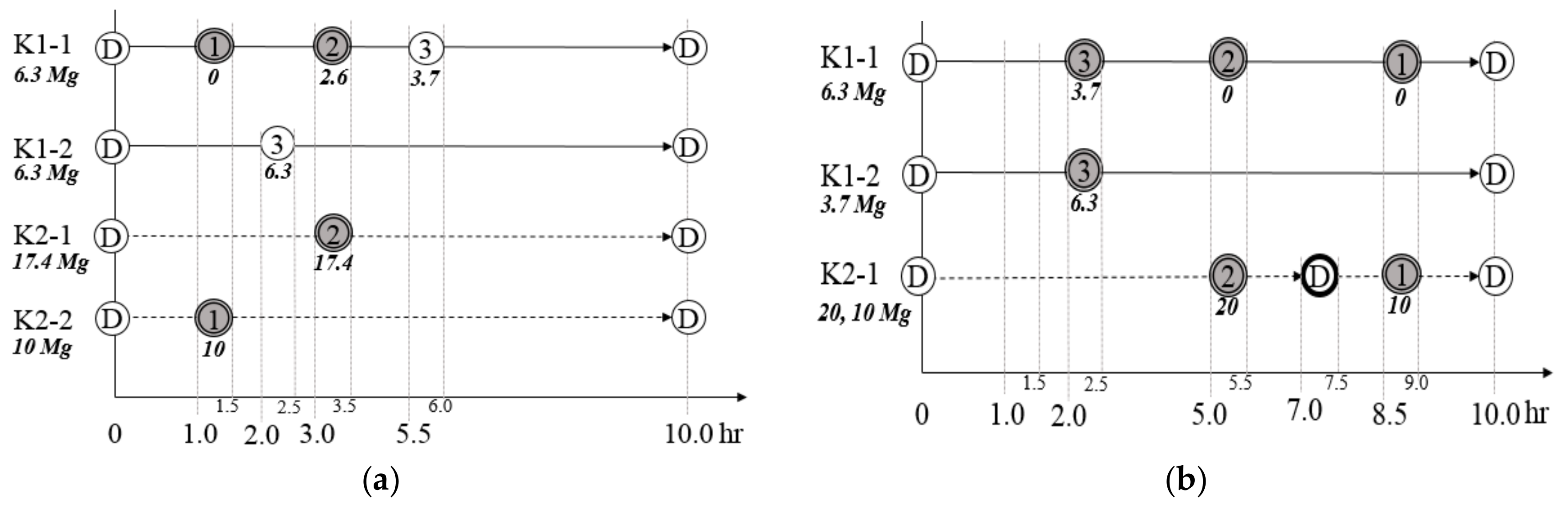
3.2. Results of Routes and Schedules

This section demonstrates how the VLRP and the MTVLRP prescribe the routes and schedules for case V30. Figure 2 depicts vehicle routes and amount of delivered bricks for case V30 prescribed by the VLRP and the MTVLRP. Each straight solid arc represents a transportation path of a loader truck; each dotted arc, that of a normal truck, respectively. K1 denotes a loader truck with a capacity of 6.3 Mg and K2, a normal truck with a capacity of 20 Mg. A curved arc at node D represents re-departure of a vehicle. Beside each customer node, the first underscored line informs its demand and other lower lines represent the amounts of bricks delivered by each vehicle.

Two loaders and two normal trucks are used in the plan prescribed by the VLRP as shown in Figure 2a. Since all customer sites have no on-site loader, loader trucks (K1-1 and K1-2) visit all customer sites. Loader truck K1-1 visits node 1 not for delivering bricks but to help normal tuck K2-2 for unloading; node 2 to deliver 2.6 Mg of bricks as well as to help normal truck K2-1 unload bricks; node 3 to deliver 3.7 Mg of bricks; and returns to the depot. K1-2 visits only node 3 to deliver 6.3 Mg of bricks. Normal trucks K2-1 and K2-2 visit nodes 2 and 1 to deliver 17.4 Mg and 10 Mg of bricks, respectively. Compared to the VLRP, the MTVLRP described in Figure 2b uses one less normal truck (i.e., two loader trucks and one normal truck). Normal truck K2-1 delivers 20 Mg of bricks to node 2, returns to the depot, and re-departs to deliver 10 Mg of bricks to node 1.

Figure 3 illustrates the detailed schedule of each vehicle. Shaded nodes stand for collaboration between loader and normal trucks for unloading bricks. It is important to note that while the length of each line segment between two nodes represents the travel time between them, the length of each last line segment from a node to the depot is not necessarily matched to the travel time because each vehicle can return to the depot any time by the end of working hours.

In the schedules of case V30 prescribed by the VLRP (Figure 3a), loader truck K1-1 arrives node 1 at 1 h and helps normal truck K2-2 to unload bricks, departs node 1 at 1.5 h, arrives node 2 at 3 h helping normal truck K2-1 to unload bricks, departs node 2 at 3.5 h, arrives node 3 at 5.5 h delivering 3.7 Mg of bricks, and returns to the depot. Since each loader truck can deliver bricks independently, customer 3 receives delivered bricks by both loader trucks K1-1 and K1-2 at different times. On the contrary, normal trucks K2-1 and K2-2 visit nodes 1 and 2 with loader truck K1-1 in the same time window, respectively. Figure 3b shows the detailed schedules of two loader trucks and one normal truck for case V30 prescribed by the MTVLRP. Normal truck K2-1 delivers 20 Mg of bricks to node 2, returns to the depot, re-depart, delivers 10 Mg of bricks to node 1, and returns to the depot. Loader truck K1-1 visits nodes 2 and 1 not for delivering products but to help normal truck K2-1 for unloading bricks.

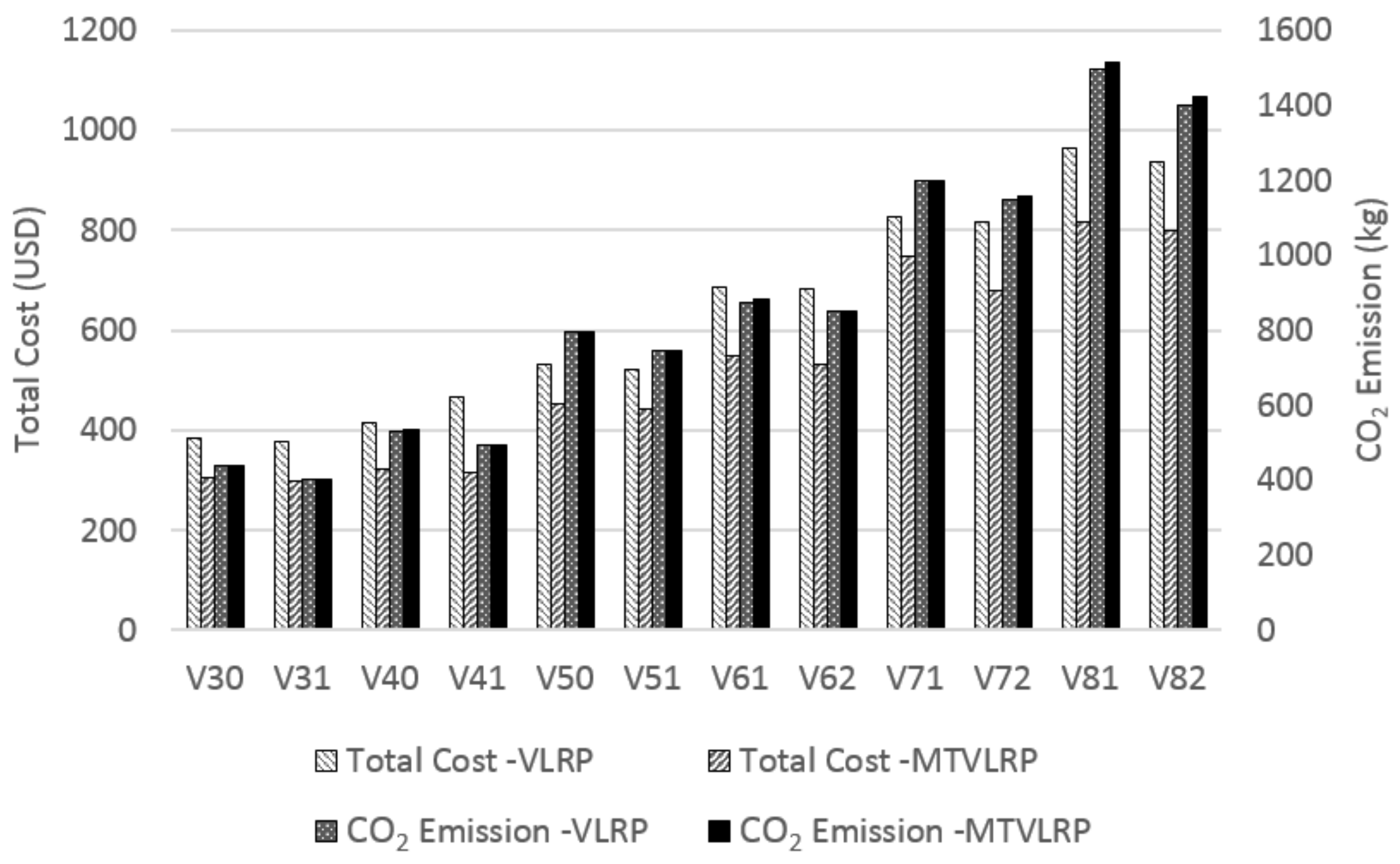
3.3. Economic and Environmental Analysis

This section analyzes the experiment results in economic and environmental perspectives. First,

Table 4. Cost analysis of the VLRP and the MTVLRP (unit: USD).

Case	Total Cost			Vehicle Cost			Operating Cost
	VLRP	MTVLRP	∆ 1	VLRP	MTVLRP	∆ 1	VLRP	MTVLRP	∆ 1
V30	385.1	305.1	−20.8%	300.0	220.0	−26.7%	85.1	85.1	0.0%
V31	376.6	296.6	−21.2%	300.0	220.0	−26.7%	76.6	76.6	0.0%
V40	413.7	323.7	−21.8%	310.0	220.0	−29.0%	103.7	103.7	0.0%
V41	465.1	315.1	−32.3%	370.0	220.0	−40.5%	95.1	95.1	0.0%
V50	532.7	452.7	−15.0%	380.0	300.0	−21.1%	152.7	152.7	0.0%
V51	522.5	442.5	−15.3%	380.0	300.0	−21.1%	142.5	142.5	0.0%
V61	687.0	548.9	−20.1%	520.0	380.0	−26.9%	167.0	168.9	1.1%
V62	681.1	531.1	−22.0%	520.0	370.0	−28.8%	161.1	161.1	0.0%
V71	827.6	747.6	−9.7%	600.0	520.0	−13.3%	227.6	227.6	0.0%
V72	817.4	679.3	−16.9%	600.0	460.0	−23.3%	217.4	219.3	0.9%
V81	962.8	816.3	−15.2%	680.0	530.0	−22.1%	282.8	286.3	1.2%
V82	934.8	798.6	−14.6%	670.0	530.0	−20.9%	264.8	268.6	1.5%

¹ ∆ = (MTVLRP-VLRP)/VLRP.

gives the total cost and its breakdown into the vehicle cost (i.e., vehicle cost) and the operating cost (i.e., the sum of the travel and waiting costs) for 12 cases. The first column gives the name of each case. The group of columns 2–4 shows the total cost prescribed by the VLRP (column 1), the MTVLRP (column 2), and the cost reduction percentage which is calculated by (MTVLRP-VLRP)/VLRP. The groups of columns 5–7 and 8–10 are the vehicle cost and the operating cost, respectively. The column structures of the vehicle cost and operating cost groups are the same as that of the total cost group.

In all cases, the MTVLRP outperforms the VLRP by reducing the total costs of 112.4 USD on average, which is 18.7% less than the VLRP. The average daily cost saving of 112.4 USD implies that compared to the VLRP, the MTVLRP may reduce annually 35,068 USD of the total delivery cost (i.e., 112.4 USD * 6 days per week * 52 weeks per year = 35,068 USD per year). Such cost reduction attributes mainly to the less vehicle costs (i.e., −25% reduction on average) from multiple utilization (i.e., multi trips) of vehicles even though a few cases (i.e., V61, V72, V81, and V82) show a slight increase (i.e., 0.4% on average) of the operating cost. Thus, even though there is a trade-off between reducing the vehicle and the operating costs, the reduction in the vehicle cost is much more significant than the slight increase in the operating cost. It is also important to note that, for the cases with the same number of customer sites (e.g., V30 and V31 or V71 and V72), cases having more on-site loaders (i.e., V31, V41, V51, V62, V72, V82) end up with less total cost than those having no (i.e., V30, V40, V50,) or less on-site loaders (i.e., V61, V71, V81). For example, the total costs of V31 and V72 are less than those of V30 and V71, respectively.

Second, to investigate the environmental effect emitted by vehicles, we analyze the amount of CO₂ emissions for studied cases. Based on the assumption that the CO₂ emission is related only to fuel consumptions by vehicles, we calculate CO₂ emission from both travel and idle times. We employ the conversion rate of 2347.7 g of CO₂ per liter according to [26]. Since the travel speed of a loader truck is 60 km per hour, and its fuel consumption during travel is 0.17 L per km, its total fuel consumption for one-hour travel is 10 L which is equivalent to 23,477 g of CO₂. Similarly, for a normal truck, its travel speed and fuel consumption during travel are 60 km per hour and 0.2 L per kilometer, respectively. Thus, it consumes 12 L of fuels for one-hour travel which is converted to 28,172 g of CO₂.

Also, according to [27], the fuel consumption rate of a medium heavy truck at idle is estimated at 3.18 L per hour. Based on the best available data we collected, we assume that both a loader and a normal truck consume fuels similarly at idle. However, it is important to note that the capacity of a loader truck (i.e., 6.3 Mg) is smaller than that of a normal truck (i.e., 20 Mg). Also, the mini crane mounted on a loader truck may not significantly increase the fuel consumption. Thus, the idling fuel consumption of a loader truck can be considered as covering both unloading operations and normal idling, while that of a normal truck, only normal idling. Hence, the CO₂ emission for one-hour idle is 7465 g of CO₂, which is calculated by 3.18 L per hour * 2347.7 g of CO₂ per liter, for both types of trucks.

Since the types of possible on-site unloaders could be diverse according to the machinery type employed at a construction site (e.g., tower crane and forklift), considering such different circumstances at construction sites would be out of the scope of this paper. Therefore, we assume that an on-site loader may emit the same amount of CO₂ to that of a loader truck. Also, this assumption may not affect our analysis for comparing the VLRP and the MTVLRP because the required unloading time for the same amount of bricks using an on-site loader is the same in both models.

Table 5. Operating times and CO₂ emission by the VLRP and the MTVLRP.

Case	Total Travel Time (hour)				Total Idle Time (hour)				Total CO2 Emission (kg)
	VLRP		MTVLRP		VLRP		MTVLRP		VLRP	MTVLRP	∆ 1
	Loader	Normal	Loader	Normal	Loader	Normal	Loader	Normal
V30	10.5	6.0	10.5	6.0	2.0	1.0	2.0	1.0	438	438	0.0%
V31	6.5	8.0	6.5	8.0	1.5	1.0	1.5	1.0	400	400	0.0%
V40	9.5	10.0	14.5	6.0	2.0	1.5	2.5	1.0	531	536	0.9%
V41	10.5	8.0	10.5	8.0	2.0	1.0	2.0	1.0	494	494	0.0%
V50	14.5	15.0	14.5	15.0	2.5	2.0	2.5	2.0	797	797	0.0%
V51	12.5	15.0	12.5	15.0	2.0	2.0	2.0	2.0	746	746	0.0%
V61	17.5	15.0	15.5	17.0	3.0	2.0	2.5	2.5	871	880	1.1%
V62	16.5	15.0	16.5	15.0	2.5	2.0	2.5	2.0	851	851	0.0%
V71	21.5	23.0	21.5	23.0	3.5	2.5	3.5	2.5	1198	1198	0.0%
V72	19.5	23.0	17.5	25.0	3.0	2.5	2.5	3.0	1147	1156	0.8%
V81	29.0	27.0	25.0	31.0	4.0	3.0	3.5	3.5	1494	1513	1.3%
V82	27.5	25.0	23.0	29.5	3.5	3.0	3.0	3.5	1399	1420	1.5%

¹ ∆ = (MTVLRP-VLRP)/VLRP.

presents total travel and idle times, and total CO₂ emission converted from those times. The first column is the name of each case. The first group of columns 2–5 shows the total travel times of each type of trucks prescribed by the VLRP (columns 2 and 3) and the MTVLRP (columns 4 and 5. Similarly, the second group of columns 6–9 gives the total idle times of each type of trucks prescribed by the VLRP (columns 6 and 7) and the MTVLRP (columns 8 and 9). The last group of columns 10–12 provides the total CO₂ emission converted from travel and idle times for the VLRP (column 10), the MTVLRP (column 11), and the CO₂ emission increase percentage which is calculated by (MTVLRP-VLRP)/VLRP.

The tiny difference in the operating costs between the VLRP and the MTVLRP in Table 4 is related to the almost same travel and idle times in Table 5. Therefore, the total CO₂ emission converted from the fuel consumption for traveling and idling are almost the same between the VLRP and the MTVLRP. The average increase of CO₂ emission by the MTVLRP compared to the VLRP is 0.5% which is almost negligible. The slight increase in travel and idle times in the MTVLRP compared to the VLRP is due to the terms in their objective functions: i.e., the VLRP minimizes only travel and waiting costs while the MTVLRP minimizes not only travel and waiting costs but also vehicle cost.

4. Discussion

In order to compare the economic and environmental effects between the VLRP and the MTVLRP, Figure 4 provides the total cost and the CO₂ emission together of each case. The bar chart in Figure 4 shows total costs, and the line chart shows CO₂ emissions. As total cost increases, CO₂ emission increases as well. In all cases, the cost reduction by the MTVLRP is significant while the increase in CO₂ emission is almost negligible. In other words, incorporating the multi-trip element into the delivery planning will create substantial economic benefits while keeping environmental effect at the almost same level. Since such an economic benefit can be acquired without worsening environmental effect, the developed MTVLRP will be able to be used as a sustainable decision support tool for many small brick manufacturers to deliver their products.

In addition, it may be interesting to note that large brick manufacturers may also be interested in using the MTVLRP for larger business cases (i.e., a larger number of customers). However, our preliminary computational test for large-scale instances (e.g., more than ten customers) identifies that CPLEX, one of currently available best commercial optimization solvers, might not be sufficient to find optimal solutions within an appropriate time duration (e.g., 1 h). Thus, to handle a larger number of customers, specialized solution algorithms may need to be developed to solve large-scale problems in the future.

5. Conclusions

The proposed mathematical model addresses the MTVLRP, a new variant of the heterogeneous VRP. To the best of our knowledge, this is the first model to deal with collaborative routing with different types of vehicles allowing multi-trips of vehicles. Brick plant managers can use our mathematical model to plan the most cost-effective delivery schedules and to estimate the required number of each type of vehicle without making noticeable ill-impact to the environment.

The case studies demonstrate the use of our model as a decision support tool based on a set of data we have been able to gather from public sources to represent a specific business case of the brick industry in the Middle East. The results show that the MTVLRP has significant economic benefits compared to the VLRP by reducing the required number of vehicles while keeping environmental effect at almost the same level. The proposed model is found to be applicable to real-world problems with a readily available standard computing set-up.

Future research can extend this study in several ways. First, specialized solution algorithms may need to be developed to solve large-scale instances, which could handle a larger number of customers and help large brick manufacturers to cope with larger business cases. Second, it will be beneficial to apply the developed model to other real-world problems. For example, the second-generation biofuel producers need to collect and transport biomass in large packages, which require special machinery for loading from the fields to a specific warehouse or a biorefinery [28]. In accordance with an increasing demand for environmentally friendly energy sources, the biofuel industry may be one of the promising application domains. Lastly, it is possible to integrate real-time traffic conditions to reflect more realistic travel times on the truck roads, which can translate into costs for maintaining more reliable brick delivery management systems.

References

1. Chao, I.M. A tabu search method for the truck and trailer routing problem. Comput. Oper. Res. 2002, 29, 33–51. [Google Scholar] [CrossRef]
2. Derigs, U.; Pullmann, M.; Vogel, U. Truck and trailer routing-problems, heuristics and computational experience. Comput. Oper. Res. 2013, 40, 536–546. [Google Scholar] [CrossRef]
3. Drexl, M. Synchronization in Vehicle Routing—A Survey of VRPs with Multiple Synchronization Constraints. Transp. Sci. 2012, 46, 297–316. [Google Scholar] [CrossRef]
4. Chen, L.; Langevin, A.; Lu, Z. Integrated scheduling of crane handling and truck transportation in a maritime container terminal. Eur. J. Oper. Res. 2013, 225, 142–152. [Google Scholar] [CrossRef]
5. An, H.; Byon, Y.J. Vehicle loader routing problem. In Proceedings of the 2016 Institute of Industrial and Systems Engineers Annual Conference & Expo, Anaheim, CA, USA, 22–25 May 2016. [Google Scholar]
6. Jabali, O.; Leus, R.; Van Woensel, T.; Kok, T. Self-imposed time windows in vehicle routing problems. OR Spectr. 2015, 37, 331–352. [Google Scholar] [CrossRef]
7. Dantzig, G.B.; Ramser, J.H. The truck dispatching problem. Manag. Sci. 1959, 6, 80–91. [Google Scholar] [CrossRef]
8. Desrochers, M.; Desrosiers, J.; Solomon, M. A new optimization algorithm for the vehicle routing problem with time windows. Oper. Res. 1992, 40, 342–354. [Google Scholar] [CrossRef]
9. Renaud, J.; Laporte, G.; Boctor, F.F. A tabu search heuristic for the multi-depot vehicle routing problem. Comput. Oper. Res. 1996, 23, 229–235. [Google Scholar] [CrossRef]
10. Wassan, N.A.; Nagy, G. Vehicle routing problem with deliveries and pickups: Modelling issues and meta-heuristics solution approaches. Int. J. Trans. 2014, 2, 95–110. [Google Scholar] [CrossRef]
11. Koç, C.; Bektaş, T.; Jabali, O.; Laporte, G. Thirty years of heterogeneous vehicle routing. Eur. J. Oper. Res. 2016, 249, 1–21. [Google Scholar] [CrossRef]
12. Brandao, J. A Decision Support System and Algorithms for the Vehicle Routing and Scheduling Problem. Ph.D. Thesis, Lancaster University, Lancaster, UK, 1994, unpublished. [Google Scholar]
13. Salhi, S. The Integration of Routing into the Location-Allocation and Vehicle Composition Problems. Ph.D. Thesis, University of Lancaster, Lancaster, UK, 1987, unpublished. [Google Scholar]
14. Brandao, J.; Mercer, A. A tabu search algorithm for the multi-trip vehicle routing and scheduling problem. Eur. J. Oper. Res. 1997, 100, 180–191. [Google Scholar] [CrossRef]
15. Koc, C.; Karaoglan, I. A branch and cut algorithm for the vehicle routing problem with multiple use of vehicles. In Proceedings of the 41st International Conference on Computers & Industrial Engineering, Los Angeles, CA, USA, 23–25 October 2011; pp. 554–559. [Google Scholar]
16. Mingozzi, A.; Roberti, R.; Toth, P. An exact algorithm for the multitrip vehicle routing problem. INFORMS J. Comput. 2013, 25, 193–207. [Google Scholar] [CrossRef]
17. Hernandez, F.; Feillet, D.; Giroudeau, R.; Naud, O. A new exact algorithm to solve the multi-trip vehicle routing problem with time windows and limited duration. Q. J. Oper. Res. 2014, 12, 235–259. [Google Scholar] [CrossRef]
18. Zhang, Y.; Qi, M.; Miao, L.; Wu, G. A generalized multi-depot vehicle routing problem with replenishment based on LocalSolver. Int. J. Ind. Eng. Comput. 2015, 6, 81–98. [Google Scholar] [CrossRef]
19. Cattaruzza, D.; Absi, N.; Feillet, D. The multi-trip vehicle routing problem with time windows and release dates. Transp. Sci. 2016, 50, 676–693. [Google Scholar] [CrossRef]
20. Braekers, K.; Ramaekers, K.; Nieuwenhuyse, I.V. The vehicle routing problem: State of the art classification and review. Comput. Ind. Eng. 2016, 99, 300–313. [Google Scholar] [CrossRef]
21. Hwang, T.; Ouyang, Y. Urban freight truck routing under stochastic congestion and emission considerations. Sustainability 2015, 7, 6610–6625. [Google Scholar] [CrossRef]
22. Ji, S.; Sun, Q. Low-carbon planning and design in B & R logistics service: A case study of an E-commerce big data platform in China. Sustainability 2017, 9, 2052. [Google Scholar] [CrossRef]
23. Guo, F.; Liu, Q.; Liu, D.; Guo, Z. On production and green transportation coordination in a sustainable global supply chain. Sustainability 2017, 9, 2071. [Google Scholar] [CrossRef]
24. Hajibabai, L.; Nourbakhsh, S.M.; Ouyang, Y.; Peng, F. Network routing of snowplow with resource replenishment and plowing priorities formulation, algorithm, and application. Transp. Res. Rec. 2014, 2440, 16–25. [Google Scholar] [CrossRef]
25. HAOY. Available online: https://xzhaoyi.en.alibaba.com/?spm=a2700.8304367.topnav.1.a23b70b5a8duFX (accessed on 4 May 2018).
26. U.S. Department of Transportation. Light-duty vehicle greenhouse gas emission standards and corporate average fuel economy standards. Fed. Regist. 2010, 75, 25324–25728. [Google Scholar]
27. Fact #861 23 February 2015 Idle Fuel Consumption for Selected Gasoline and Diesel Vehicles. Available online: Energy.gov/eere/vehicles/fact-861-february-23-2015-idle-fuel-consumption-selected-gasoline-and-diesel-vehicles (accessed on 20 February 2018).
28. An, H.; Searcy, S.W. Economic and energy evaluation of a logistics system based on biomass modules. Biomass Bioenergy 2012, 46, 190–202. [Google Scholar] [CrossRef]
Figure 1. Example plan of multi-trip vehicle loader routing problem.
Sustainability 10 01427 g001
Figure 2. Route networks for V30: (a) by VLRP; (b) by MTVLRP.
Sustainability 10 01427 g002
Figure 3. Delivery schedules of V30: (a) by VLRP; (b) by MTVLRP.
Sustainability 10 01427 g003
Figure 4. Total Cost vs. CO2 Emissions.
Sustainability 10 01427 g004