Impact of Human Actions on Building Energy Performance: A Case Study in the United Arab Emirates (UAE)


Abstract
:1. Introduction
2. Methodology
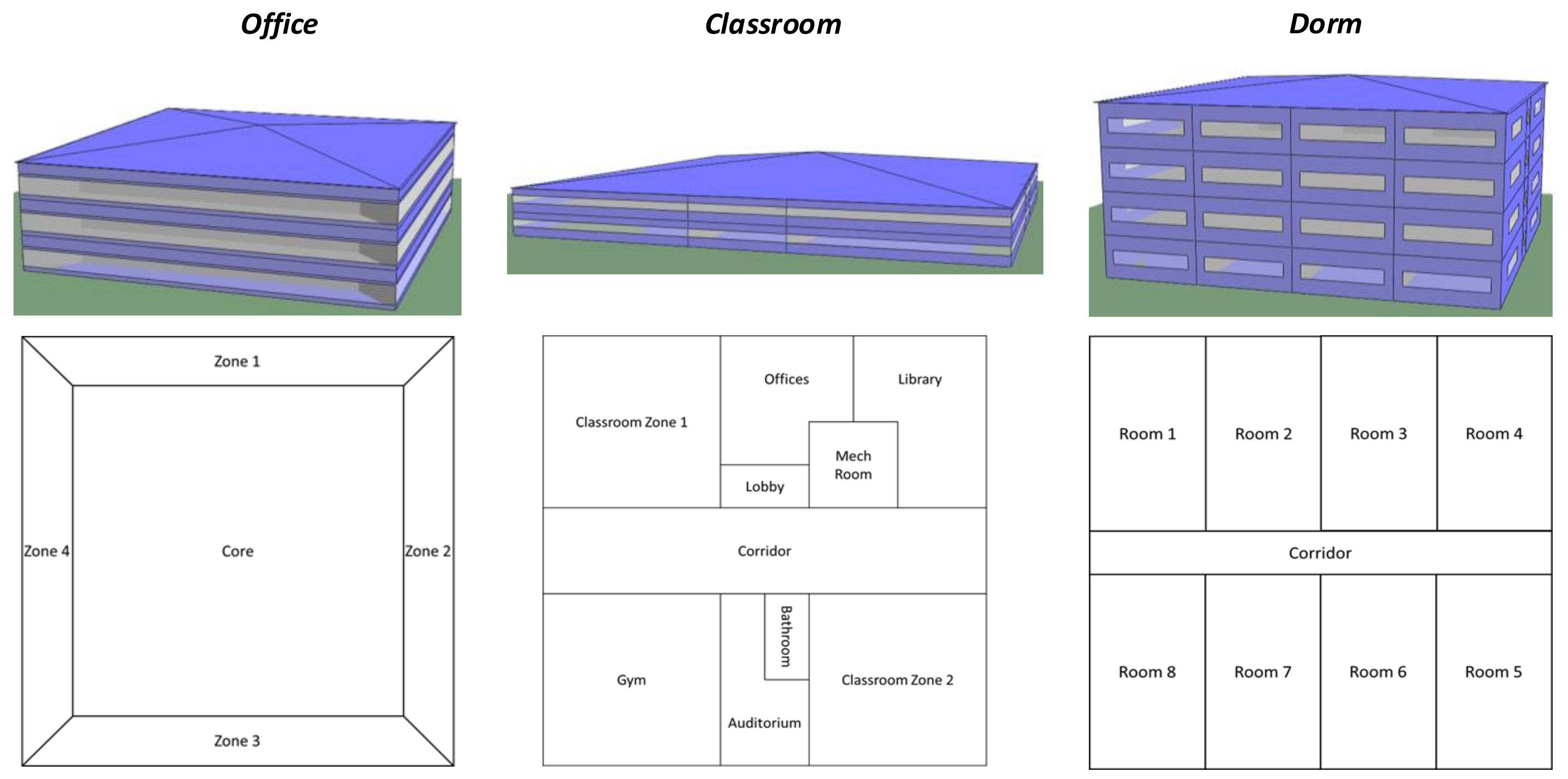
2.1. Data Gathering
2.2. Energy Modeling
2.3. Parametric Variation
2.3.1. Method 1: Differential Analysis
2.3.2. Method 2: Fractional Factorial Analysis
2.3.3. Method 3: Monte Carlo Analysis
3. Results
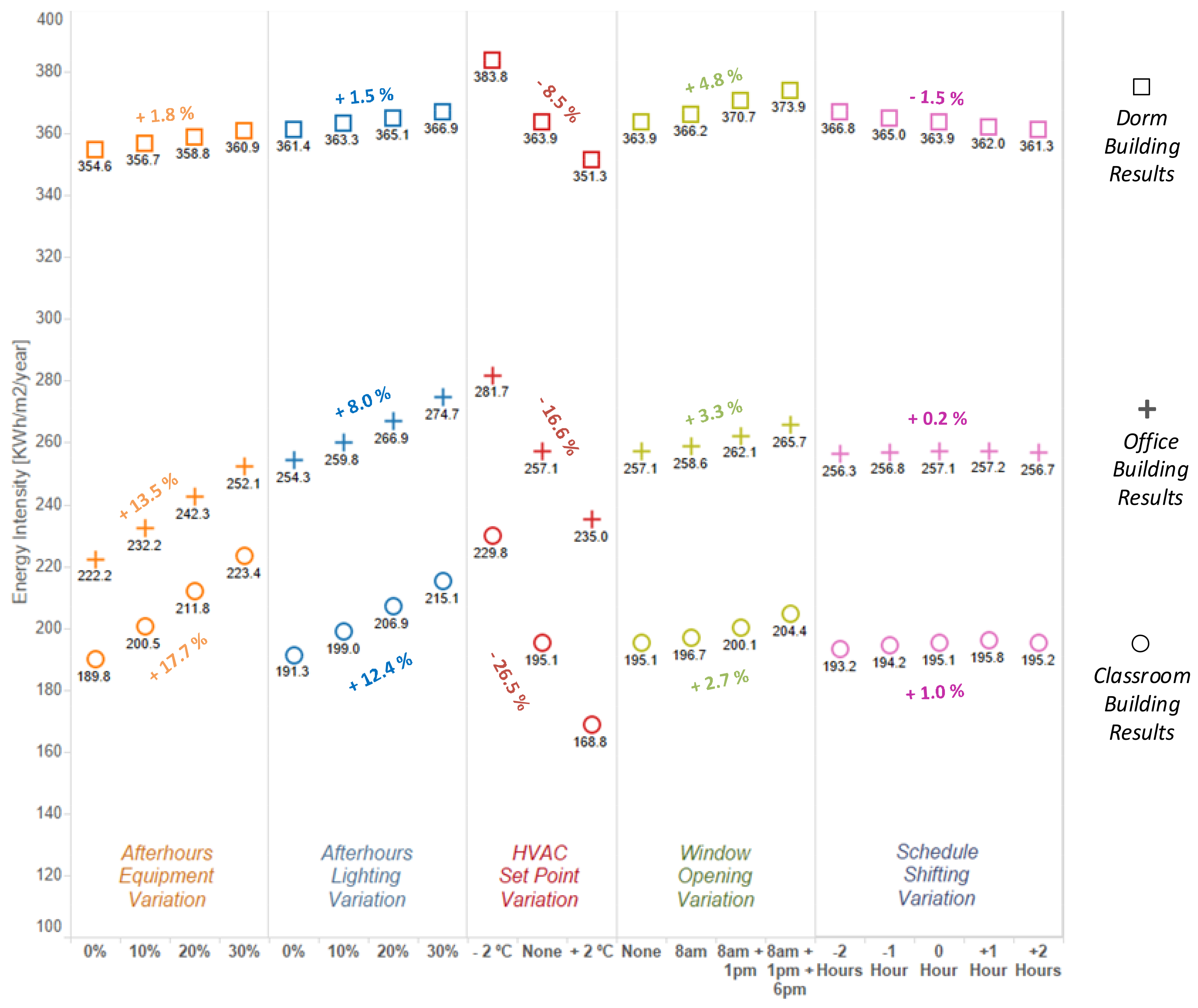
3.1. Differential Analysis Results
3.2. Fractional Factorial Analysis Results
3.3. Monte Carlo Analysis Results
4. Discussion
5. Conclusions
Author Contributions
Conflicts of Interest
Appendix A

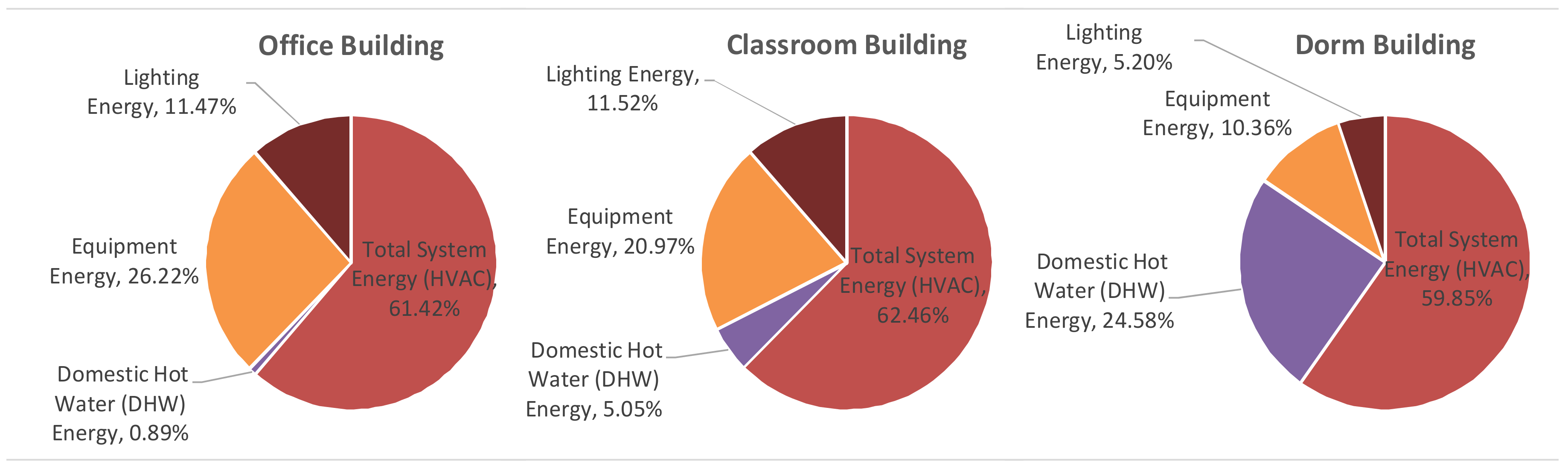
| Office Building | Classroom Building | Dorm Building | |||||||
|---|---|---|---|---|---|---|---|---|---|
| Week-Days | Week-End Day 1 | Week-End Day 2 | Week-Days | Week-End Day 1 | Week-End Day 2 | Week-Days | Week-End Day 1 | Week-End Day 2 | |
| 1 h | 0 | 0 | 0 | 0 | 0 | 0 | 1 | 1 | 1 |
| 2 h | 0 | 0 | 0 | 0 | 0 | 0 | 1 | 1 | 1 |
| 3 h | 0 | 0 | 0 | 0 | 0 | 0 | 1 | 1 | 1 |
| 4 h | 0 | 0 | 0 | 0 | 0 | 0 | 1 | 1 | 1 |
| 5 h | 0 | 0 | 0 | 0 | 0 | 0 | 1 | 1 | 1 |
| 6 h | 0 | 0 | 0 | 0 | 0 | 0 | 1 | 1 | 1 |
| 7 h | 0.1 | 0.1 | 0.05 | 0 | 0 | 0 | 1 | 1 | 1 |
| 8 h | 0.2 | 0.1 | 0.05 | 0.05 | 0 | 0 | 0.9 | 0.9 | 0.9 |
| 9 h | 0.95 | 0.3 | 0.05 | 0.75 | 0.1 | 0 | 0.4 | 0.4 | 0.4 |
| 10 h | 0.95 | 0.3 | 0.05 | 0.9 | 0.1 | 0 | 0.25 | 0.25 | 0.25 |
| 11 h | 0.95 | 0.3 | 0.05 | 0.9 | 0.1 | 0 | 0.25 | 0.25 | 0.25 |
| 12 h | 0.95 | 0.3 | 0.05 | 0.8 | 0.1 | 0 | 0.25 | 0.25 | 0.25 |
| 13 h | 0.5 | 0.1 | 0.05 | 0.8 | 0.1 | 0 | 0.25 | 0.25 | 0.25 |
| 14 h | 0.95 | 0.1 | 0.05 | 0.8 | 0 | 0 | 0.25 | 0.25 | 0.25 |
| 15 h | 0.95 | 0.1 | 0.05 | 0.8 | 0 | 0 | 0.25 | 0.25 | 0.25 |
| 16 h | 0.95 | 0.1 | 0.05 | 0.45 | 0 | 0 | 0.25 | 0.25 | 0.25 |
| 17 h | 0.95 | 0.1 | 0.05 | 0.15 | 0 | 0 | 0.3 | 0.3 | 0.3 |
| 18 h | 0.3 | 0.05 | 0.05 | 0.05 | 0 | 0 | 0.5 | 0.5 | 0.5 |
| 19 h | 0.1 | 0.05 | 0 | 0.15 | 0 | 0 | 0.9 | 0.9 | 0.9 |
| 20 h | 0.1 | 0 | 0 | 0.2 | 0 | 0 | 0.9 | 0.9 | 0.9 |
| 21 h | 0.1 | 0 | 0 | 0.2 | 0 | 0 | 0.9 | 0.9 | 0.9 |
| 22 h | 0.1 | 0 | 0 | 0.1 | 0 | 0 | 1 | 1 | 1 |
| 23 h | 0.05 | 0 | 0 | 0 | 0 | 0 | 1 | 1 | 1 |
| 24 h | 0.05 | 0 | 0 | 0 | 0 | 0 | 1 | 1 | 1 |
References
- US Department of Energy (DOE). Energy Efficiency Trends in Residential and Commercial Buildings; DOE: Washington, DC, USA, 2010.
- International Energy Agency (IEA). Energy Efficiency; IEA: Paris, France, 2015. [Google Scholar]
- Afshari, A.; Nikolopoulou, C.; Martin, M. Life-cycle analysis of building retrofits at the urban scale—A case study in united arab emirates. J. Sustain. 2014, 6, 453–473. [Google Scholar] [CrossRef]
- Executive Affairs Authority. Demand-Side management. In Technical Report; Executive Affairs Authority: Abu Dhabi, UAE, 2009. [Google Scholar]
- United Nations Environment Programme (UNEP). Buildings Can Play Key Role In Combating Climate Change. UNEP, 2007. Available online: https://news.un.org/en/story/2007/03/213932-building-sector-can-play-key-role-combating-global-warming-un-report-says (accessed on 18 March 2018).
- Hoes, P.; Hensen, J.L.M.; Loomans, M.; De Vries, B.; Bourgeois, D. User behavior in whole building simulation. Energy Build. 2009, 41, 295–302. [Google Scholar] [CrossRef]
- Turner, C.; Frankel, M. Energy Performance of LEED for New Construction Buildings; New Buildings Institute: Vancouver, WA, USA, 2008. [Google Scholar]
- US Department of Energy (DOE). Building Energy Software Directory; DOE: Washington, DC, USA, 2011.
- Yudelson, J. Greening Existing Buildings; McGraw-Hill: New York, NY, USA, 2010. [Google Scholar]
- Roth, K.W.; Westphalen, D.; Feng, M.Y.; Llana, P.; Quartararo, L. Energy Impact of Commercial Building Controls and Performance Diagnostics: Market Characterization, Energy Impact of Building Faults and Energy Savings Potential. Prepared by TAIX LLC for the US Department of Energy. 2005. Available online: https://s3.amazonaws.com/zanran_storage/www.tiaxllc.com/ContentPages/42428345.pdf (accessed on 18 March 2018).
- Granderson, J.; Piette, M.A.; Rosenblum, B.; Hu, L. Energy Information Handbook: Applications for Energy-Efficient Building Operations; Lawrence Berkeley National Laboratory (LBNL): Berkeley, CA, USA, 2009. [Google Scholar]
- Masoso, O.T.; Grobler, L.J. The dark side of occupants’ behaviour on building energy use. Energy Build. 2010, 42, 173–177. [Google Scholar] [CrossRef]
- Sanchez, M.; Webber, C.; Brown, R.; Busch, J.; Pinckard, M.; Roberson, J. Space Heaters, Computers, Cell Phone Chargers: How Plugged in Are Commercial Buildings? Lawrence Berkeley National Laboratory: Berkeley, CA, USA, 2007.
- Webber, C.A.; Roberson, J.A.; McWhinney, M.C.; Brown, R.E.; Pinckard, M.J.; Busch, J.F. After-hours power status of office equipment in the USA. Energy 2006, 31, 2823–2838. [Google Scholar] [CrossRef]
- Yan, D.; Hong, T.; Dong, B.; Mahdavi, A.; D’Oca, S.; Gaetani, I.; Feng, X. IEA EBC Annex 66: Definition and simulation of occupant behavior in buildings. Energy Build. 2017, 156, 258–270. [Google Scholar] [CrossRef]
- Delzendeh, E.; Wu, S.; Lee, A.; Zhou, Y. The impact of occupants’ behaviours on building energy analysis: A research review. Renew. Sustain. Energy Rev. 2017, 80, 1061–1071. [Google Scholar] [CrossRef]
- Khosrowpour, A.; Gulbinas, R.; Taylor, J.E. Occupant workstation level energy-use prediction in commercial buildings: Developing and assessing a new method to enable targeted energy efficiency programs. Energy Build. 2016, 127, 1133–1145. [Google Scholar] [CrossRef]
- Ryu, S.H.; Moon, H.J. Development of an occupancy prediction model using indoor environmental data based on machine learning techniques. Build. Environ. 2016, 107, 1–9. [Google Scholar] [CrossRef]
- Ouf, M.; Issa, M.; Merkel, P. Analysis of real-time electricity consumption in Canadian school buildings. Energy Build. 2016, 128, 530–539. [Google Scholar] [CrossRef]
- Heydarian, A.; Carneiro, J.P.; Gerber, D.; Becerik-Gerber, B. Immersive virtual environments, understanding the impact of design features and occupant choice upon lighting for building performance. Build. Environ. 2015, 89, 217–228. [Google Scholar] [CrossRef]
- Yan, D.; O’Brien, W.; Hong, T.; Feng, X.; Gunay, H.B.; Tahmasebi, F.; Mahdavi, A. Occupant behavior modeling for building performance simulation: Current state and future challenges. Energy Build. 2015, 107, 264–278. [Google Scholar] [CrossRef]
- Pisello, A.L.; Castaldo, V.L.; Piselli, C.; Fabiani, C.; Cotana, F. How peers’ personal attitudes affect indoor microclimate and energy need in an institutional building: Results from a continuous monitoring campaign in summer and winter conditions. Energy Build. 2016, 126, 485–497. [Google Scholar] [CrossRef]
- Schakib-Ekbatan, K.; Cakıcı, F.Z.; Schweiker, M.; Wagner, A. Does the occupant behavior match the energy concept of the building? Analysis of a German naturally ventilated office building. Build. Environ. 2015, 84, 142–150. [Google Scholar] [CrossRef]
- D’Oca, S.; Fabi, V.; Corgnati, S.P.; Andersen, R.K. Effect of thermostat and window opening occupant behavior models on energy use in homes. Build. Simul. 2014, 7, 683–694. [Google Scholar] [CrossRef]
- Azar, E.; Menassa, C.C. A comprehensive analysis of the impact of occupancy parameters in energy simulation of office buildings. J. Energy Build. 2012, 55, 841–853. [Google Scholar] [CrossRef]
- Azar, E.; Menassa, C.C. A comprehensive framework to quantify energy savings potential from improved operations of commercial building stocks. Energy Policy 2014, 67, 459–472. [Google Scholar] [CrossRef]
- Arup Consultants. Pearls design system new buildings. In Technical Report; Urban Planning Council: Abu Dhabi, UAE, 2010. [Google Scholar]
- American Society of Heating Refrigerating and Air-Conditioning Engineers (ASHRAE). Energy Standard for Buildings Except Low-Rise Residential Buildings; ASHRAE 90.1-2013; ASHRAE Inc.: Atlanta, GA, USA, 2013. [Google Scholar]
- Deru, M.; Field, K.; Studer, D.; Benne, K.; Griffith, B.; Torcellini, P.; Liu, B.; Halverson, M.; Winiarski, D.; Rosenberg, M. U.S. department of energy commercial reference building models of the national building stock. In Technical Report; National Renewable Energy Laboratory (NREL): Golden, CO, USA, 2011. [Google Scholar]
- Gowri, K.; Winiarski, D.; Jarnagin, R. Infiltration Modeling Guidelines for Commercial Building Energy Analysis; Pacific Northwest National Laboratory (PNNL): Richland, WA, USA, 2009.
- EnergyPlus. Weather Data by Location. Energy Plus Website. 2015. Available online: https://energyplus.net/weather-location/asia_wmo_region_2/ARE/ARE_Abu.Dhabi.412170_IWEC (accessed on 18 March 2018).
- Afshari, A.; Friedrich, L. A proposal to introduce tradable energy savings certificates in the emirate of Abu Dhabi. Renew. Sustain. Energy Rev. 2016, 55, 1342–1351. [Google Scholar] [CrossRef]
- Ameer, B.; Krarti, M. Impact of subsidization on high energy performance designs for Kuwaiti residential buildings. Energy Build. 2016, 116, 249–262. [Google Scholar] [CrossRef]
- Sgouridis, S.; Abdullah, A.; Griffiths, S.; Saygin, D.; Wagner, N.; Gielen, D.; McQueen, D. RE-mapping the UAE’s energy transition: An economy-wide assessment of renewable energy options and their policy implications. Renew. Sustain. Energy Rev. 2016, 55, 1166–1180. [Google Scholar] [CrossRef]
- US Energy Information Administration (EIA). Commercial Buildings Energy Consumption Survey (CBECS); EIA: Washington, DC, USA, 2003.
- Tian, W. A review of sensitivity analysis methods in building energy analysis. Renew. Sustain. Energy Rev. 2013, 20, 411–419. [Google Scholar] [CrossRef]
- Hamby, D.M. A review of techniques for parameter sensitivity analysis of environmental models. Environ. Monit. Assess. 1994, 32, 135–154. [Google Scholar] [CrossRef] [PubMed]
- Langner, M.R.; Henze, G.P.; Corbin, C.D.; Brandemuehl, M.J. An investigation of design parameters that affect commercial high-rise office building energy consumption and demand. J. Build. Perform. Simul. 2012, 5, 313–328. [Google Scholar] [CrossRef]
- Box, G.E.; Hunter, J.S.; Hunter, W.G. Statistics for Experimenters: Design, Innovation, and Discovery; Wiley-Interscience: New York, NY, USA, 2005; Volume 2. [Google Scholar]
- Nguyen, A.; Relter, S. A performance comparison of sensitivity analysis methods for building energy models. Build. Simul. 2015, 8, 651–664. [Google Scholar] [CrossRef]
- Lomas, K.J.; Eppel, H. Sensitivity analysis techniques for building thermal simulation programs. Energy Build. 1992, 19, 21–44. [Google Scholar] [CrossRef]
- Wang, L.; Mathew, P.; Pang, X. Uncertainties in energy consumption introduced by building operations and weather for a medium-size office building. Energy Build. 2012, 53, 152–158. [Google Scholar] [CrossRef]
- Bornatico, R.; Hüssy, J.; Witzig, A.; Guzzella, L. Surrogate modeling for the fast optimization of energy systems. Energy 2013, 57, 653–662. [Google Scholar] [CrossRef]
- Rijal, H.B.; Tuohy, P.; Humphreys, M.A.; Nicol, J.F.; Samuel, A.; Clarke, J. Using results from field surveys to predict the effect of open windows on thermal comfort and energy use in buildings. Energy Build. 2007, 39, 823–836. [Google Scholar] [CrossRef]
- Rijal, H.B.; Tuohy, P.; Humphreys, M.A.; Nicol, J.F.; Samuel, A.; Raja, I.A.; Clarke, J. Development of adaptive algorithms for the operation of windows, fans, and doors to predict thermal comfort and energy use in Pakistani buildings. ASHRAE Trans. 2008, 114, 555–573. [Google Scholar]
- Asadi, S.; Amiri, S.; Mottahedi, M. On the development of multi-linear regression analysis to assess energy consumption in the early stages of building design. Energy Build. 2014, 85, 246–255. [Google Scholar] [CrossRef]
- Catalina, T.; Virgone, J.; Blanco, E. Development and validation of regression models to predict monthly heating demand for residential buildings. Energy Build. 2008, 40, 1825–1832. [Google Scholar] [CrossRef]
- Hygh, J.; DeCarolis, J.; Hill, D.; Ranji Ranjithan, S. Multivariate regression as an energy assessment tool in early building design. Build. Environ. 2012, 57, 165–175. [Google Scholar] [CrossRef]
- Lam, J.; Wan, K.; Liu, D.; Tsang, C. Multiple regression models for energy use in air-conditioned office buildings in different climates. Energy Convers. Manag. 2010, 51, 2692–2697. [Google Scholar] [CrossRef]
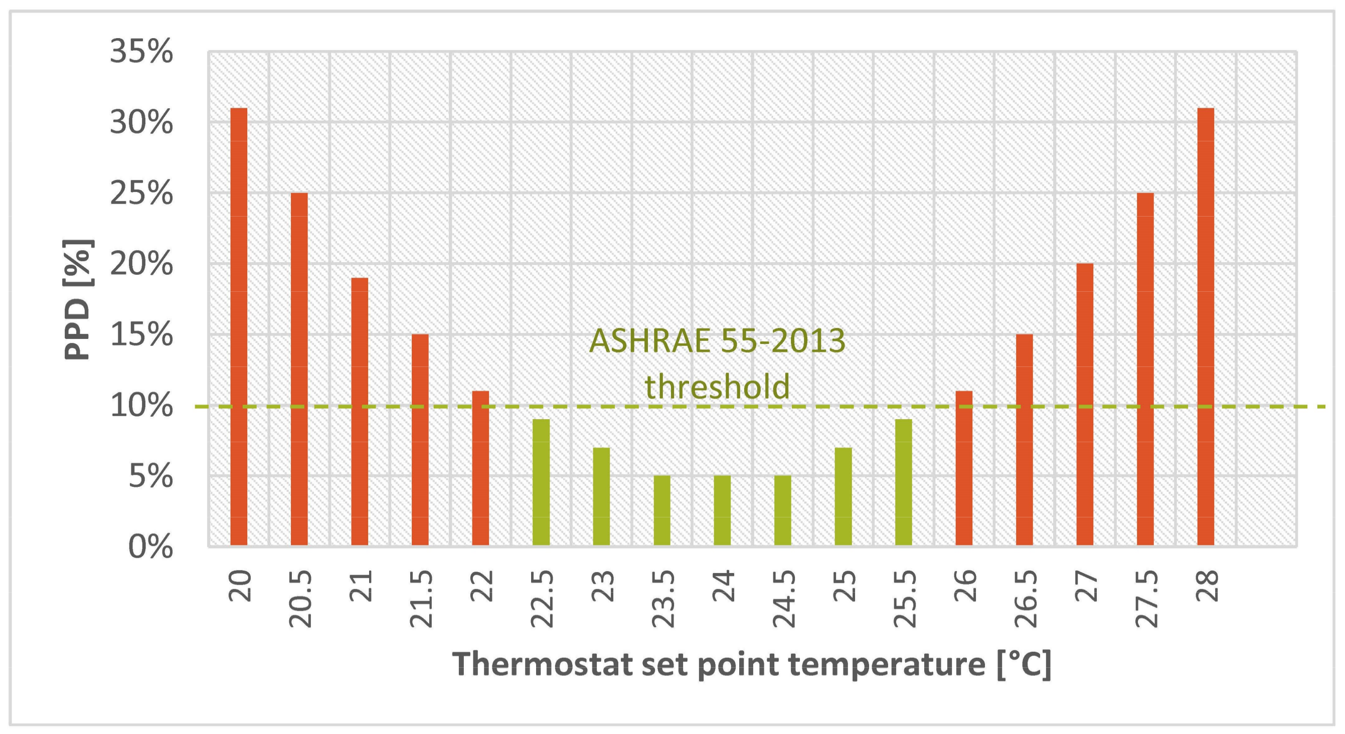
- American Society of Heating Refrigerating and Air-Conditioning Engineers (ASHRAE). Thermal Environment Conditions for Human Occupancy; ASHRAE 55-2013; ASHRAE Inc.: Atlanta, GA, USA, 2013. [Google Scholar]
- Hoy, T.; Schiavon, S.; Piccioli, A.; Cheung, T.; Moon, D.; Steinfeld, K. CBE Thermal Comfort Tool; Center for the Built Environment, University of California: Berkeley, CA, USA, 2017. [Google Scholar]
- Berbari, G.J.; Shakkour, S.; Hashem, F. Fresh air-handling units: Comparison and design guide. ASHRAE J. 2007, 49, 34. [Google Scholar]
- Karjalainen, S. Gender differences in thermal comfort and use of thermostats in everyday thermal environments. Build. Environ. 2007, 42, 1594–1603. [Google Scholar] [CrossRef]
- Kalmár, F. An indoor environment evaluation by gender and age using an advanced personalized ventilation system. Build. Serv. Eng. Res. Technol. 2017, 38, 505–521. [Google Scholar] [CrossRef]
- Nakano, J.; Tanabe, S.; Kimura, K. Differences in perception of indoor environment between Japanese and non-japanese workers. Energy Build. 2002, 34, 615–621. [Google Scholar] [CrossRef]
- Indraganti, M. Behavioural adaptation and the use of environmental controls in summer for thermal comfort in apartments in India. Energy Build. 2010, 42, 1019–1025. [Google Scholar] [CrossRef]
- Chen, J.; Taylor, J.E.; Wei, H. Modeling building occupant network energy consumption decision-making: The interplay between network structure and conservation. Energy Build. 2012, 47, 515–524. [Google Scholar] [CrossRef]
- Peschiera, G.; Taylor, J.E. The impact of peer network position on electricity consumption in building occupant networks utilizing energy feedback systems. Energy Build. 2012, 49, 584–590. [Google Scholar] [CrossRef]
- Peschiera, G.; Taylor, J.E.; Siegel, J.A. Response–Relapse patterns of building occupant electricity consumption following exposure to personal, contextualized and occupant peer network utilization data. Energy Build. 2010, 42, 1329–1336. [Google Scholar] [CrossRef]


| Parameter | Units | Office | Classroom | Dorm |
|---|---|---|---|---|
| Typical Total Floor Area [27,29] | m2 | 4982 | 19,592 | 3135 |
| Building Width (calculated) | m | 40.8 | 100.0 | 28.0 |
| Building Length (calculated) | m | 40.8 | 100.0 | 28.0 |
| Floor Height [29] | m | 4.0 | 4.0 | 3.1 |
| Number of Stories [29] | Floors | 3 | 2 | 4 |
| Location | ----- | Abu Dhabi | Abu Dhabi | Abu Dhabi |
| Glazing Fraction Window-to-Wall Ratio (WWR) [27,29] | ----- | 50% | 33% | 15% |
| People Density [28] | m2/person | 18.6 | 3.7 | 9.3 |
| Minimum Fresh Air [27] | L/s/person | 10 | 10 | 2 |
| Infiltration Rate [30] | Air changes per hour (ACH) | 0.5 | 0.5 | 0.7 |
| Equipment Intensity [27,28] | W/m2 | 15.0 | 15.0 | 6.4 |
| Lighting Intensity [27,28] | W/m2 | 10.0 | 10.7 | 6.6 |
| Domestic Hot Water (DHW) [28] | L/Person | 3.8 | 6.8 | 48.1 |
| Wall U-Values [3] | W/m2·K | 1.7 | 1.7 | 1.7 |
| Roof U-Values [3] | W/m2·K | 0.5 | 0.5 | 0.5 |
| Glazing U-Values [27] | W/m2·K | 2.4 | 2.4 | 2.4 |
| Occupants Maximum Sensible Gain [28] | W/Person | 73.3 | 73.3 | 73.3 |
| Occupants Maximum Latent Gain [28] | W/Person | 58.6 | 58.6 | 58.6 |
| Occupancy, Equipment, Lighting, and HVAC Profiles [28] (Refer to Appendix A for more details) | ----- | Table 5-J Schedule A | Table G-K School Occupancy | Table 5-M Schedule D |
| HVAC Occupied [27] & Unoccupied Set points | °C | Occupied: 22 Unoccupied: 24 | Occupied: 22 Unoccupied: 24 | Occupied: 22 Unoccupied: 24 |
| Cooling System Type [29] | ----- | PACU (packaged air conditioning unit) | Chiller—air cooled | PACU—SS (Split System) |
| Air Distribution [29] | ----- | MZ VAV (multi-zone variable air volume) | MZ VAV | SZ CAV (single-zone constant air volume) |
| Building | Year Built | Floors | Percent Glazed (Front/Right) | Glazing Type (Front/Right) | Tinting Type (Front/Right) | Shading (Front/Right) |
|---|---|---|---|---|---|---|
| Office #1 | 1990–1994 | 2 | 80–100%/<20% | Single/n/a | None/n/a | No/No |
| Office #2 | 2000–2004 | 2 | 20–40%/n/a | Single/n/a | Tinted/n/a | No/n/a |
| Office #3 | 2005–2007 | 2 | <20%/<20% | Single/n/a | Tinted/n/a | No/No |
| Office #4 | 2008–2012 | 2 | <20%/<20% | Dble./Dble. | Reflect./Reflect. | No/No |
| Class. #1 | 1990–1994 | 1 | 60–80%/60–80% | Single/Single | Reflect./Reflect. | Yes/Yes |
| Class. #2 | <1990 | 2 | 40–60%/40–60% | Single/Single | Tinted/Tinted | Yes/Yes |
| Class. #3 | 1990–1994 | 2 | <20%/<20% | Single/Single | Tinted/Tinted | No/Yes |
| Class.#4 | 2000–2004 | 3 | 20–40%/<20% | Single/Single | Reflect./Reflect. | No/No |
| Class. #5 | 1995–1999 | 2 | 40–60%/20–40% | Single/Single | Tinted/Tinted | Yes/Yes |
| Dorm #1 | n/a | 4 | <20%/<20% | Single/Single | Tinted/Reflect. | No/No |
| Dorm #2 | n/a | 4 | 20–40%/<20% | Dble./Single | Tinted/None | No/Yes |
| Dorm #3 | 2008–2012 | 4 | 0%/20–40% | Single/Single | None/None | No/No |
| Models | Abu Dhabi Buildings | CBECS Buildings | |||
|---|---|---|---|---|---|
| Energy Intensity [kWh/m2/Year] | Energy Intensity [kWh/m2/Year] | Difference with Models [%] | Energy Intensity [kWh/m2/Year] | Difference with Models [%] | |
| Office | 257.1 | 243.1 | +5.4 | 278.1 | −8.1 |
| Classroom | 195.1 | 205.1 | −5.2 | 191.8 | +1.7 |
| Dorm | 363.9 | 354.5 | +2.6 | 331.2 | +9.0 |
| Parameter | Scenarios |
|---|---|
| Equipment use during unoccupied periods | 0%, 10%, 20%, and 30% |
| Lighting use during unoccupied periods | 0%, 10%, 20%, and 30% |
| Shifting schedules | Baseline schedule varied by ± 1 h and ± 2 h |
| Window opening | 1 h (8 a.m.), 2 h (8 a.m. + 1 p.m.), 3 h (8 a.m. + 1 p.m. + 6 p.m.) |
| HVAC occupied set point | Baseline value (22 °C) ± 2 °C |
| HVAC unoccupied set point | Baseline value (24 °C) ± 2 °C |
| HVAC occupied and unoccupied aet points simultaneously | Baseline values (22 °C and 24 °C) ± 2 °C |
| Parameter | Base | Test |
|---|---|---|
| Equipment & Lighting | Unoccupied 0% | Unoccupied 30% |
| Window Opening | None | 3 h (8 a.m. + 1 p.m. + 6 p.m.) |
| Shifting HVAC set points by 2 °C | 22 °C (occupied) 24 °C (unoccupied) | 20 °C (occupied) 22 °C (unoccupied) |
| Shifting Schedules | None | −2 h |
| Parameter | Range |
|---|---|
| Equipment use during unoccupied periods | 0%, 10%, 20% and 30% |
| Lighting use during unoccupied periods | 0%, 10%, 20% and 30% |
| Window Opening | None, 1 h (8 a.m.), 2 h (8 a.m. + 1 p.m.), 3 h (8 a.m. + 1 p.m. + 6 p.m.) |
| Shifting HVAC set points | Occupied Period: 20 °C, 21 °C, 22 °C, 23 °C, and 24 °C Unoccupied Period: 22 °C, 23 °C, 24 °C, 25 °C, and 26 °C |
| Shifting Schedules | −2 h, −1 h, None, +1 h, +2 h |
| Run | Parameter | Energy Intensity (kWh/m2/Year) | |||||
|---|---|---|---|---|---|---|---|
| -A- (EL) | -B- (WO) | -C- (HVAC) | -D- (SS) | Office | Classroom | Dorm | |
| 1 | Base | Base | Base | Base | 257.1 | 195.1 | 363.9 |
| 2 | Base | Base | Base | Test | 256.3 | 193.2 | 366.8 |
| 3 | Base | Base | Test | Base | 281.7 | 229.8 | 383.8 |
| 4 | Base | Base | Test | Test | 281.4 | 229.3 | 386.2 |
| 5 | Base | Test | Base | Base | 265.7 | 204.4 | 373.9 |
| 6 | Base | Test | Base | Test | 265.5 | 203.0 | 376.6 |
| 7 | Base | Test | Test | Base | 291.3 | 238.5 | 394.8 |
| 8 | Base | Test | Test | Test | 291.8 | 237.7 | 396.6 |
| 9 | Test | Base | Base | Base | 270.0 | 242.8 | 363.9 |
| 10 | Test | Base | Base | Test | 259.6 | 227.2 | 365.0 |
| 11 | Test | Base | Test | Base | 294.8 | 277.1 | 383.9 |
| 12 | Test | Base | Test | Test | 284.8 | 262.8 | 384.4 |
| 13 | Test | Test | Base | Base | 278.8 | 251.4 | 374.0 |
| 14 | Test | Test | Base | Test | 268.9 | 236.4 | 374.8 |
| 15 | Test | Test | Test | Base | 304.4 | 285.1 | 394.8 |
| 16 | Test | Test | Test | Test | 295.4 | 270.8 | 394.8 |
| A&B [EL&WO] | A&C [EL&HVAC] | A&D [EL&SS] | B&C [WO&HVAC] | B&D [WO&SS] | C&D [HVAC&SS] | ||||||
|---|---|---|---|---|---|---|---|---|---|---|---|
| Office Building Results | |||||||||||
| 277.97 | 277.97 | 277.97 | 277.97 | 277.97 | 277.97 | ||||||
| ab | 269.13 | ac | 261.15 | ad | 273.95 | bc | 260.75 | bd | 275.90 | cd | 267.90 |
| AB | 286.88 | AC | 294.85 | AD | 277.18 | BC | 295.73 | BD | 280.40 | CD | 288.35 |
| Ab | 277.30 | Ac | 269.33 | Ad | 287.00 | Bc | 269.73 | Bd | 285.05 | Cd | 293.05 |
| aB | 278.58 | aC | 286.55 | aD | 273.75 | bC | 285.68 | bD | 270.53 | cD | 262.58 |
| 0.000 | 0.000 | −0.035 | 0.004 | 0.003 | 0.002 | ||||||
| Classroom Building Results | |||||||||||
| 236.54 | 236.54 | 236.54 | 236.54 | 236.54 | 236.54 | ||||||
| ab | 211.85 | ac | 198.93 | ad | 216.95 | bc | 214.58 | bd | 236.20 | cd | 223.43 |
| AB | 260.93 | AC | 273.95 | AD | 249.30 | BC | 258.03 | BD | 236.98 | CD | 250.15 |
| Ab | 252.48 | Ac | 239.45 | Ad | 264.10 | Bc | 223.80 | Bd | 244.85 | Cd | 257.63 |
| aB | 220.90 | aC | 233.83 | aD | 215.80 | bC | 249.75 | bD | 228.13 | cD | 214.95 |
| −0.006 | −0.002 | −0.058 | −0.004 | 0.001 | 0.004 | ||||||
| Dorm Building Results | |||||||||||
| 379.89 | 379.89 | 379.89 | 379.89 | 379.89 | 379.89 | ||||||
| ab | 375.18 | ac | 370.30 | ad | 379.10 | bc | 364.90 | bd | 373.88 | cd | 368.93 |
| AB | 384.60 | AC | 389.48 | AD | 379.75 | BC | 395.25 | BD | 385.70 | CD | 390.5 |
| Ab | 374.30 | Ac | 369.43 | Ad | 379.15 | Bc | 374.83 | Bd | 384.38 | Cd | 389.33 |
| aB | 385.48 | aC | 390.35 | aD | 381.55 | bC | 384.58 | bD | 375.60 | cD | 370.80 |
| 0.000 | 0.000 | −0.005 | 0.002 | −0.001 | −0.002 | ||||||
© 2018 by the authors. Licensee MDPI, Basel, Switzerland. This article is an open access article distributed under the terms and conditions of the Creative Commons Attribution (CC BY) license (http://creativecommons.org/licenses/by/4.0/).
Share and Cite
Al Amoodi, A.; Azar, E. Impact of Human Actions on Building Energy Performance: A Case Study in the United Arab Emirates (UAE). Sustainability 2018, 10, 1404. https://doi.org/10.3390/su10051404
Al Amoodi A, Azar E. Impact of Human Actions on Building Energy Performance: A Case Study in the United Arab Emirates (UAE). Sustainability. 2018; 10(5):1404. https://doi.org/10.3390/su10051404
Chicago/Turabian StyleAl Amoodi, Ahmed, and Elie Azar. 2018. "Impact of Human Actions on Building Energy Performance: A Case Study in the United Arab Emirates (UAE)" Sustainability 10, no. 5: 1404. https://doi.org/10.3390/su10051404
APA StyleAl Amoodi, A., & Azar, E. (2018). Impact of Human Actions on Building Energy Performance: A Case Study in the United Arab Emirates (UAE). Sustainability, 10(5), 1404. https://doi.org/10.3390/su10051404