Flowchart on Choosing Optimal Method of Observing Transverse Dispersion Coefficient for Solute Transport in Open Channel Flow

Abstract

There are a number of methods for observing and estimating the transverse dispersion coefficient in an analysis of the solute transport in open channel flow. It may be difficult to select an optimal method to calculate dispersion coefficients from tracer data among numerous methodologies. A flowchart was proposed in this study to select an appropriate method under the transport situation of either time-variant or steady condition. When making the flowchart, the strengths and limitations of the methods were evaluated based on its derivation procedure which was conducted under specific assumptions. Additionally, application examples of these methods on experimental data were illustrated using previous works. Furthermore, the observed dispersion coefficients in a laboratory channel were validated by using transport numerical modeling, and the simulation results were compared with the experimental results from tracer tests. This flowchart may assist in choosing the better methods for determining the transverse dispersion coefficient in various river mixing situations.

1. Introduction

The longitudinal and transverse dispersion coefficients are the major parameters of the two-dimensional solute transport model in an open channel flow. Because these coefficients can determine the peak concentration and the spreading area of the solute, we must pay careful attention when calculating the values of these coefficients in modelling processes. Conventionally, the model parameters of dispersion coefficients can be observed by the ‘‘inverse method”, which estimates parameters inversely by matching numerical solutions acquired from a numerical model to measured mixing data from either field or laboratory experiments. Many models, unfortunately, suffer from approximation errors that manifest themselves as numerical diffusion. Estimated dispersion coefficients based on numerical models are sometimes unrealistic, and may not be transferable to other sites or problems [1]. Thus, reliable methods have been proposed that avoid the uncertainties associated with simulations and reduce the computational burden associated with numerical models, while facilitating the direct determination of dispersion coefficients [2].

In general, the choice of methodologies on determining the transverse dispersion coefficient for solute mixing in an open channel depends on whether tracer concentration data is available or not. The observing method calculates the dispersion coefficient with the concentration data from tracer experiments or field measurements. The estimating method predicts the coefficient using basic geometrics and hydraulics without tracer concentration data [3]. The representative methodologies for the observing method are routing procedures and moment-based methods. It may also be difficult to select an optimal method to determine dispersion coefficients for a given situation among observing methods. This study suggests how to choose the better equation for calculating the transverse dispersion coefficient with available tracer data. The criteria for selecting a suitable method under various situations of mixing are presented by a flowchart.

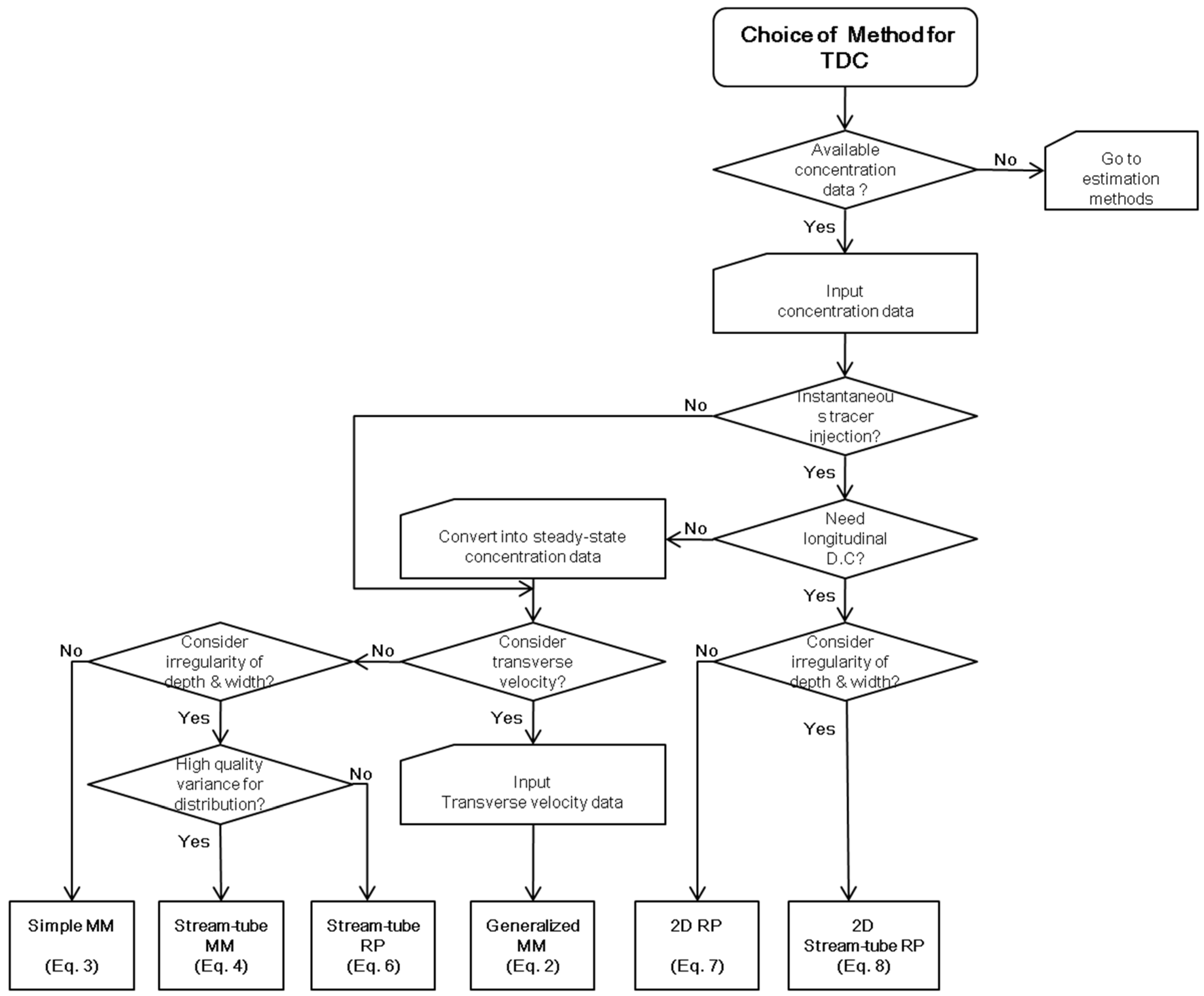
2. Materials and Methods

In two-dimensional river mixing, mixing data can be classified into two types; time-variant data and steady data. The former can be acquired from a transient concentration situation by injecting a tracer instantaneously. The latter is acquired under steady concentration conditions from a continuous injection of a tracer. Most field studies based on continuous tracer injection had been conducted during 1970–80s. When the channel discharge and the solute inflow rate are both steady, the downstream plume also eventually becomes steady; time derivative terms vanish. Furthermore, under this condition the longitudinal mixing term may be dropped in the two-dimensional mass transport model. It is well known that dispersive transport is small relative to convective transport in a unidirectional flow [4]. Moment-based methods were derived in such conditions and were commonly used to calculate the transverse dispersion coefficient by researchers [4,5,6,7]. Of course, the moment-based methods also may be applied to the conditions of time-variant concentration using Beltaos’ conversion procedure [8]. In such cases, time variations within the concentration data were vanished by using a defined tracer dosage.

$$\theta (x,y)\equiv {\displaystyle {\int }_0^{\infty }C(x,y,t)dt}$$

(1)

where $\theta$ is the dosage; C is the depth-averaged concentration of a tracer; t is time; and x and y are the longitudinal transverse coordinates respectively.

The generalized moment method (generalized MM) by Holley et al. [6], which can reflect the effects of the transverse velocities and tracer impinging on the banks, for the $\theta$-equation yields.

$$D_T=\frac{1}{2}\frac{\partial }{\partial x}\left(\frac{{\displaystyle {\int }_0^{W}u\theta y^2}dy}{{\displaystyle {\int }_0^{W}u\theta dy}}\right)\left(\frac{{\displaystyle {\int }_0^{W}u\theta dy}}{{\left[\theta y\right]}_0^W-{\displaystyle {\int }_0^W\theta dy}}\right)-\frac{{\displaystyle {\int }_0^{W}v\theta ydy}}{{\left[\theta y\right]}_0^W-{\displaystyle {\int }_0^W\theta dy}}=\frac{1}{2}\frac{\partial {\sigma }_y^2}{\partial x}\frac{1}{f}-\frac{g}{f}$$

(2)

where $D_T$ is the transverse dispersion coefficients; $W$ is the channel width; ${\sigma }_y^2$ is the second moment of the transverse distribution of the concentration data; $f$ and $g$ are the terms which reflect the tracer impinging on the banks and the transverse velocities, respectively; $u$ and $v$ are the depth-averaged longitudinal and transverse velocities, respectively. We can calculate the transverse dispersion coefficient using the slope of the straight line which is fitted to the plot of variance (${\sigma }_y^2$) against longitudinal distance ($x$). The simple moment method (simple MM) by Sayre and Chang [4] can be derived from the generalized MM, Equation (2). Neglecting the transverse velocity and the tracer impinging on banks, and assuming a constant longitudinal velocity, Equation (2) becomes:

$$D_T=\frac{U}{2}\frac{\partial }{\partial x}\left(\frac{{\displaystyle {\int }_0^W\theta y^2}dy}{{\displaystyle {\int }_0^W\theta dy}}\right)=\frac{U}{2}\frac{\partial {\sigma }_y^2}{\partial x}$$

(3)

where $U$ is the reach-averaged longitudinal velocity. The stream–tube moment method (stream–tube MM) by Beltaos [7] can reflect irregularities of depth and width at rivers by using the stream–tube concept. The method is:

$$D_T=\frac{Q^2}{2\mathrm{\Psi }U{H}^2}\frac{d{\sigma }_{\eta }^2}{dx}\frac{1}{\left(1-(1-{\eta }_0)S_1-{\eta }_0{S}_0\right)}$$

(4)

where ${\sigma }_{\eta }^2$ and ${\eta }_0$ are the second and first moments of the $S-\eta$ distribution, respectively; $\eta \equiv q/Q$; q and Q are the cumulative flow and the total flow discharge, respectively; $S\equiv \theta /\mathrm{\Theta }$; $\mathrm{\Theta }={\displaystyle {\int }_0^1\theta d\eta }$; $S_0$ and $S_1$ are the normalized dosages at the left and right banks, respectively; $H$ is the mean depth; and $\mathrm{\Psi }$ is a normalized shape–velocity factor that has a range of 1.0–3.6 [7] and is defined by:

$$\mathrm{\Psi }=\frac{1}{Q}{\displaystyle {\int }_0^Q{h}^2}udq$$

(5)

These moment-based methods, however, have some restrictions in which the skewed concentration profile induced by river irregularities makes it difficult to compute a meaningful value for the second moments. This may lead to an inaccurate dispersion coefficient. Seo et al. [9] developed the stream–tube routing procedure (stream–tube RP), a routing procedure combined with the stream–tube concept to overcome the weak point of the moment-based methods. The equation is:

$$S(x_2,\eta )={\displaystyle {\int }_0^1\frac{S(x_1,\omega )}{\sqrt{4\pi B_C(x_2-x_1)}}}\exp \left(\frac{-{(\eta -\omega )}^2}{4B_C(x_2-x_1)}\right)d\omega$$

(6)

where $S(x_1,\omega )$ is the observed dosage distribution at an upstream $x_1$; $S(x_2,\eta )$ is the predicted dosage distribution at a downstream $x_2$; $B_C=\mathrm{\Psi }U{H}^2{D}_T/Q^2$; and $\omega$ is a transverse distance variable for the integration. The merit of the routing procedure is that it is relatively simple and easy in comparison to constructing numerical simulation models. The routing procedure is, of course, a type of inverse method where the dispersion coefficient is determined by trial and error until the model results agree with tracer tests or other observations.

When it is needed to acquire both the transverse dispersion and longitudinal dispersion coefficients from tracer data under time-variant concentration situation, other routing procedures should be employed to the observed dispersion coefficients. Baek et al. [10] expanded the one-dimensional equation by Fischer [11] into two-dimensional equation. The equation (2D RP) is:

$$\begin{array}{l}C(x_2,y,t)\\ ={\displaystyle {\int }_0^W{\displaystyle {\int }_{-\infty }^{\infty }\frac{C(x_1,\psi ,\tau )U}{4\pi ({\overline{t}}_2-{\overline{t}}_1)\sqrt{D_L{D}_T}}}}\exp \left(-\frac{U^2{({\overline{t}}_2-{\overline{t}}_1-t+\tau )}^2}{4D_L({\overline{t}}_2-{\overline{t}}_1)}\right)\exp \left(-\frac{{(y-\psi )}^2}{4D_T({\overline{t}}_2-{\overline{t}}_1)}\right)d\tau d\psi \end{array}$$

(7)

where $C(x_2,y,t)$ is the predicted concentration at a downstream section, $x_2$; $C(x_1,\psi ,\tau )$ is the observed concentration at a upstream section, $x_1$; ${\overline{t}}_1$ and ${\overline{t}}_2$ are the mean times of passage in sections $x_1$ and $x_2$, respectively; $\tau$ is a time variable for the integration; $\psi$ is a distance variable for the integration; $D_L$ is the longitudinal dispersion coefficient. The calculated concentration by Equation (7) is matched repeatedly with the measured concentration by changing the dispersion coefficient until the differences between two concentrations become minimized. The value for the dispersion coefficient with the least error in concentration is regarded as the observed dispersion coefficient [12].

2D RP (Equation (7)) also has limitations. It cannot reflect the irregularities of a river—such as non-uniformities of the bed and the channel width, a skewed velocity profile, meandering—and so on. To consider such irregularities, Baek and Seo [13] derived another routing procedure from Equation (7) combining with the stream–tube concept. The equation (2D stream-tube RP) is:

$$\begin{array}{l}C(x_2,\eta ,t)\\ ={\displaystyle {\int }_0^1\frac{\left[{\displaystyle {\int }_{-\infty }^{\infty }\frac{C(x_1,\omega ,\tau )U}{\sqrt{4\pi D_L({\overline{t}}_2-{\overline{t}}_1)}}\cdot \exp \left(-\frac{U^2{({\overline{t}}_2-{\overline{t}}_1-t+\tau )}^2}{4D_L({\overline{t}}_2-{\overline{t}}_1)}\right)d\tau }\right]}{\sqrt{4\pi B_C(x_2-x_1)}}}\cdot \exp \left(-\frac{{(\eta -\omega )}^2}{4B_C(x_2-x_1)}\right)d\omega \end{array}$$

(8)

where $C(x_2,\eta ,t)$ is the predicted concentration at $x_2$; and $C(x_1,\omega ,\tau )$ is the measured concentration at $x_1$. The above methods, including the moment-based method and the routing procedure, to observe the dispersion coefficients are summarized in

Table 1. Summary of observing method for dispersion coefficients in 2D mixing.

Method	Name	Researcher	Equation	Properties
Moment-based Method	Simple MM (Equation (3))	Sayre and Chang [4]	$D_T=\frac{U}{2}\frac{\partial {\sigma }_y^2}{\partial x}$	• Neglects transverse velocity and bank impinging
	Generalized MM (Equation (2))	Holley et al. [6]	$D_T=\frac{1}{2}\frac{\partial {\sigma }_y^2{}_2}{\partial x}\frac{1}{f}-\frac{g}{f}$	• Considers transverse velocity and bank impinging
	Stream-tube MM (Equation (4))	Beltaos [7]	$\begin{array}{l}{D}_T=\frac{Q^2}{2\mathrm{\Psi }U{H}^2}\frac{d{\sigma }_{\eta }^2}{dx}\\ \hspace{1em}\hspace{1em}\cdot \frac{1}{\left(1-(1-{\eta }_0)S_1-{\eta }_0{S}_0\right)}\end{array}$	• Considers irregular depth, velocity and bank impinging
Routing Procedure	2D RP (Equation (7))	Baek et al. [10]	$\begin{array}{l}C(x_2,y,t)=\\ {\displaystyle {\int }_0^W{\displaystyle {\int }_{-\infty }^{\infty }\frac{C(x_1,\psi ,\tau )U}{4\pi ({\overline{t}}_2-{\overline{t}}_1)\sqrt{D_L{D}_T}}}}\\ \cdot \exp \left(-\frac{U^2{({\overline{t}}_2-{\overline{t}}_1-t+\tau )}^2}{4D_L({\overline{t}}_2-{\overline{t}}_1)}\right)\\ \cdot \exp \left(-\frac{{(y-\psi )}^2}{4D_T({\overline{t}}_2-{\overline{t}}_1)}\right)d\tau d\psi \end{array}$	• Evaluates not only transverse dispersion but also longitudinal dispersion coefficients • Neglects irregular depth and velocity
	Stream-tube RP (Equation (6))	Seo et al. [9]	$\begin{array}{l}S(x_2,\eta )=\\ {\displaystyle {\int }_0^1\frac{S(x_1,\omega )}{\sqrt{4\pi B_C(x_2-x_1)}}}\\ \cdot \exp \left(\frac{-{(\eta -\omega )}^2}{4B_C(x_2-x_1)}\right)d\omega \end{array}$	• Considers irregular depth and velocity • Evaluates only the transverse dispersion coefficient
	2D stream-tube RP (Equation (8))	Baek and Seo [13]	$\begin{array}{l}C(x_2,\eta ,t)=\\ {\displaystyle {\int }_0^1\frac{\left[A\right]}{\sqrt{4\pi B_C(x_2-x_1)}}}\\ \cdot \exp \left(-\frac{{(\eta -\omega )}^2}{4B_C(x_2-x_1)}\right)d\omega \end{array}$$\begin{array}{l}A={\displaystyle {\int }_{-\infty }^{\infty }\frac{C(x_1,\omega ,\tau )U}{\sqrt{4\pi D_L({\overline{t}}_2-{\overline{t}}_1)}}}\\ \cdot \exp \left(-\frac{U^2{({\overline{t}}_2-{\overline{t}}_1-t+\tau )}^2}{4D_L({\overline{t}}_2-{\overline{t}}_1)}\right)d\tau \end{array}$	• Combined method of 2D RP and Stream-tube RP • Evaluates not only transverse dispersion but also longitudinal dispersion coefficients • Considers irregular depth and velocity

.

3. Results

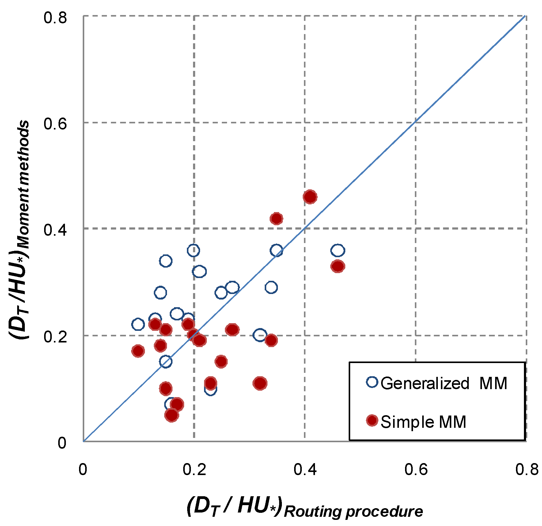
The strengths and limitations of the methods described in the previous section are obvious, as the methods were derived under specific original assumptions. Application examples may be found in previous works, such as [2,3,10,13]. Baek et al. [10] showed comparisons of the observed dispersion coefficients calculated by both the moment-based methods such as the simple MM and generalized MM and the routing procedure, 2D RP, based on tracer mixing data sets which were acquired from the artificial meandering channel with rectangular cross section. The results are depicted in Figure 1. We can see that observed values of the dispersion coefficient from the moment-based methods and the routing procedure are in the same range. More than half values resulting from the generalized MM are higher than others because this method accounts for the effect of the transverse velocity and the tracer impinging on the banks. We also deduced from this figure that the time-variant concentration condition included in the routing procedure does not affect significantly the mechanism of transverse dispersion. This is because unsteadiness was incorporated into the longitudinal dispersion term, not the transverse dispersion term as shown in Equation (7).

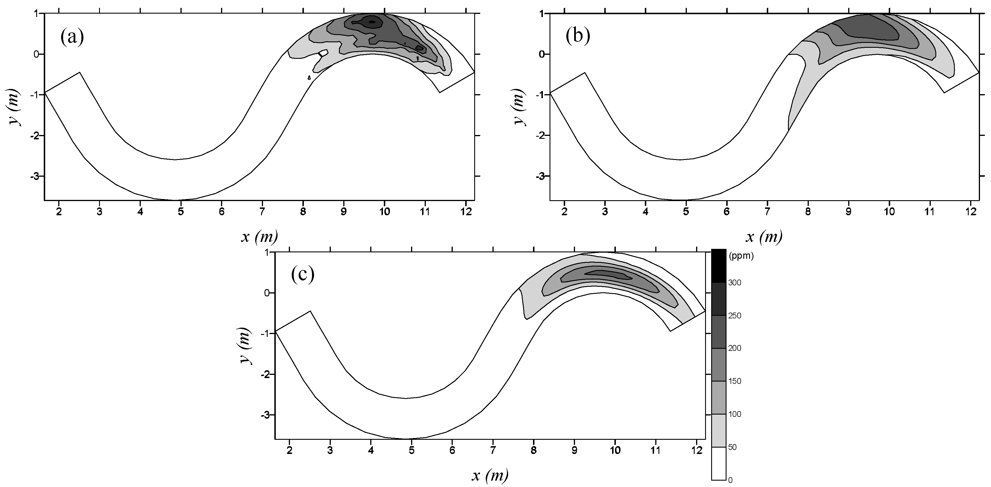
The observed dispersion coefficients in this laboratory channel were further validated by Seo et al. [2], in which they calculated the dispersion coefficients at each section based on a transport numerical modeling. According to Seo et al. [2], a finite element scheme (specifically the Petrov–Galerkin type) was used to construct a numerical model, and the simulation results from the model were verified and compared with the tracer experimental data in the laboratory curved channel. The comparison is depicted in Figure 2. Seo et al. [2] showed that the dispersion coefficient acquired directly from velocity profiles (DC1 as shown Figure 2b) supplied a more precise solution than the coefficient based on the dispersion tensor (DC2 as shown Figure 2c). Additionally, Seo et al. [2] inversely calculated the dispersion coefficient at each section based on the numerical model to reveal the spatial variations along the curved channel. The results are shown in Figure 3a. Baek and Seo [3] calculated inversely the dispersion coefficient along the identical channel by using 2D RP, as illustrated in Figure 3b. As shown in this figure, the inversely calculated values of dispersion coefficient by the numerical model and 2D RP are in good agreement with each other along the channel.

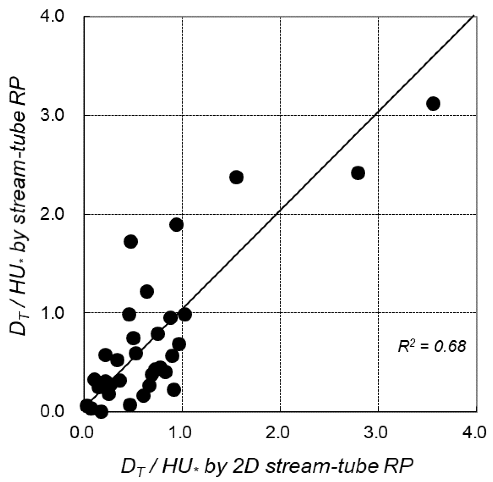
Baek and Seo [13] presented comparisons of the observed dispersion coefficients by 2D stream–tube RP and the stream–tube RP based on tracer data sets which were acquired from experiments conducted at bends of natural streams. In this study, several experimental results from tracer field tests were also added to verify and compare the two methods. Nine cases of tracer experiments were conducted at five streams in Korea. Rhodamine WT was selected as a tracer—a fluorescent dye that has been widely used for mixing study in streams—as it is conservative material and easily detectable with low background concentration [14]. Using combined dispersion data sets (Baek and Seo [13], and this study), observed dispersion coefficients by two routing procedures are compared in Figure 4. Theoretically, the values for the transverse dispersion coefficient by the two routing procedures should be identical [13]. From Figure 4, it can be seen that there is generally good agreement between values calculated by 2D stream–tube RP and those calculated by stream–tube RP, although there are somewhat scattered trends.

Recently, Baek and Seo [3] showed comparison of the observed values by the simple MM, the stream–tube MM, 2D RP, and 2D stream–tube MM based on nine experimental cases which were conducted at natural rivers, including Baek and Seo [13]. They concluded that both the stream–tube RP and 2D stream–tube RP generated reasonable dispersion coefficients values that reflected the irregularities of the river’s geometry and hydraulics.

4. Discussion

The choice of method for calculating the transverse dispersion coefficient, in general, depends on whether tracer concentration data is available or not. When concentration data sets are available, either moment-based methods or routing procedures are used for observing the transverse dispersion coefficient in two-dimensional river mixing. In case of the time-variant concentration data that was acquired under the situation of instantaneous tracer injection, both transverse dispersion and longitudinal dispersion coefficients can be provided by means of 2D RP. If it is especially necessary to reflect the irregularities of river widths, water depth, and sinuosity, the 2D stream–tube RP must be employed. In cases of steady-state concentration conditions with no longitudinal information, the transverse dispersion coefficient may only be calculated by means of either a moment-based method or a routing procedure. When transverse velocity data is available, the generalized MM must be used. When channel irregularities must be taken into account, the stream–tube MM or RP should be adopted. The simple MM is used for reference because it is simple, but less precise comparatively. Note that the moment-based methods should not be applied to concentration distributions which have a severe skewed variance. The criteria for selecting a suitable method under the various situations for calculating the dispersion coefficients with available tracer data are summarized using a flowchart in Figure 5.

5. Conclusions

There are various observing methods which calculate the transverse dispersion coefficient in a two-dimensional solute transport model at open channel flow with given tracer dispersion data. The condition of the tracer concentration field also is classified into time-variant and steady-state situations. When it is needed to obtain both the transverse and longitudinal dispersion coefficients in the time-variant concentration field, routing procedures should be adopted to compute dispersion coefficients. Baek et al. [10] expanded a one-dimensional routing equation into a two-dimensional equation for applying 2D mixing at the intermediate-field under a time-variant concentration situation. Furthermore, Baek and Seo [10] derived 2D stream–tube RP from the solution of the transport equation combined with the stream–tube concept to reflect irregularities of rivers. Under the steady-state concentration condition which was established by continuous tracer injection, the methods most frequently used are moment-based methods. In this case, time variations within the concentration data are negated, so that the longitudinal dispersion properties are also eliminated. The generalized MM can reflect the effects of the transverse velocities and tracer impinging on the banks. Neglecting the transverse velocity and the tracer impinging on banks, and assuming a constant longitudinal velocity, the generalized MM becomes the simple MM. The stream–tube MM proposed by Beltaos [7] can reflect irregularities of the depth and channel width of rivers by using the stream–tube concept. In the absence of any mixing data, either theoretical or empirical equations may be used to estimate the transverse dispersion coefficient based on basic geometric and hydraulic data sets. This topic, the so-called estimating method, is beyond the scope of this study. A flowchart for the suitable selection of estimating methods to be used in the case of no mixing data has been already presented by Baek and Seo [15].

References

1. Piasecki, M.; Katopodes, N.D. Identification of stream dispersion coefficients by adjoint sensitivity method. J. Hydraul. Eng. 1999, 125, 714–724. [Google Scholar]
2. Seo, I.W.; Lee, M.E.; Baek, K.O. 2D modeling of heterogeneous dispersion in meandering channels. J. Hydraul. Eng. 2008, 134, 196–204. [Google Scholar] [CrossRef]
3. Baek, K.O.; Seo, I.W. On the methods for determining the transverse dispersion coefficient in river mixing. Adv. Water Resour. 2016, 90, 1–9. [Google Scholar] [CrossRef]
4. Sayre, W.W.; Chang, F.M. A Laboratory Investigation of Open Channel Dispersion Processes for Dissolved, Suspended, and Floating Dispersants; Professional Paper No. 433-E; U.S. Geological Survey: Reston, WV, USA, 1968.
5. Holley, E.R. Transverse Mixing in Rivers; Laboratory Report No. S-132; Delft Hydraulics Lab.: Delft, The Netherlands, 1971. [Google Scholar]
6. Holley, E.R.; Siemons, J.; Abraham, G. Some aspects of analyzing transverse diffusion in rivers. J. Hydraul. Res. 1972, 10, 27–57. [Google Scholar] [CrossRef]
7. Beltaos, S. Transverse mixing tests in natural streams. J. Hydraul. Div. ASCE 1980, 106, 1607–1625. [Google Scholar]
8. Beltaos, S. Evaluation of transverse mixing coefficients from slug tests. J. Hydraul. Res. 1975, 13, 351–360. [Google Scholar] [CrossRef]
9. Seo, I.W.; Baek, K.O.; Jeon, T.M. Analysis of transverse mixing in natural streams under slug tests. J. Hydraul. Res. 2006, 44, 350–362. [Google Scholar] [CrossRef]
10. Baek, K.O.; Seo, I.W.; Jung, S.J. Evaluation of transverse dispersion coefficient in meandering channel from transient tracer tests. J. Hydraul. Eng. 2006, 132, 1021–1032. [Google Scholar] [CrossRef]
11. Fischer, H.B. Dispersion predictions in natural streams. J. Sanit. Eng. Div. ASCE 1968, 94, 927–943. [Google Scholar]
12. Fischer, H.B.; List, E.J.; Koh, R.C.Y.; Imberger, J.; Brooks, N.H. Mixing in Inland and Coastal Waters; Academic Press: New York, NY, USA, 1979. [Google Scholar]
13. Baek, K.O.; Seo, I.W. Routing procedures for observed dispersion coefficients in two-dimensional river mixing. Adv. Water Resour. 2010, 33, 1551–1559. [Google Scholar] [CrossRef]
14. Rowinski, P.M.; Chrzanowski, M.M. Influence of selected fluorescent dyes on small aquatic organisms. Acta Geophys. 2011, 59, 91–109. [Google Scholar] [CrossRef]
15. Baek, K.O.; Seo, I.W. Estimation of the transverse dispersion coefficient for two-dimensional models of mixing in natural streams. J. Hydro-Environ. Res. 2017, 15, 67–74. [Google Scholar] [CrossRef]
Figure 1. Comparisons of observed values for transverse dispersion coefficient by routing procedure and moment-based methods in a laboratory channel (modified from Baek et al. [10]).
Sustainability 10 01332 g001
Figure 2. Tracer concentration contour (Case 213, t = 21 s) in a laboratory meandering channel; (a) experimental result; (b) numerical result using DC1; (c) numerical result using DC2 (after Seo et al. [2]).
Sustainability 10 01332 g002
Figure 3. Calculation of transverse dispersion coefficient along a laboratory channel; (a) by 2D RP (after Baek and Seo, [3]); (b) by numerical model (after Seo et al. [2]).
Sustainability 10 01332 g003
Figure 4. Comparisons of observed values for transverse dispersion coefficient by stream–tube RP and 2D stream–tube RP in natural streams.
Sustainability 10 01332 g004
Figure 5. Flow chart for choosing an optimal method for observing dispersion coefficients in two-dimensional river mixing with tracer concentration data.
Sustainability 10 01332 g005