The System Dynamics (SD) Analysis of the Government and Power Producers’ Evolutionary Game Strategies Based on Carbon Trading (CT) Mechanism: A Case of China

Abstract

Climate warming caused by carbon emissions is one of the most serious problems faced by human beings, and the carbon trading (CT) mechanism is an effective way to promote carbon emission reduction and achieve green and low-carbon development. Scholars have mainly studied the impact of CT on the energy economy system, and few scholars studied the game process and behavior strategies of government and power producers in the implementation of a CT mechanism. This paper will fill this gap. This paper firstly constructs the evolutionary game model of government and power producers based on CT, and then simulates the evolutionary process of game behavior strategies by establishing a system dynamics (SD) model, and finally studies the influence of government controllable key factors on system stability. The combination of evolutionary game and SD in our study not only clearly reveals the complex and dynamic evolution process of game models under bounded rationality, but also provides a qualitative and quantitative simulation platform for analyzing the dynamic game process between government and power producers. The results show that: (1) There is no evolutionarily stable strategy (ESS) in the game system between government and power producers under CT, and the system evolution is characterized by periodicity; (2) When the government implements dynamic subsidies or punitive measures, the mixed strategy of the game system has ESS; (3) Reducing the unit subsidy and raising the unit fine can both promote the participation of power producers in CT, but the former increases the probability of government supervision; thus, it is best to increase the fines when the government makes strategic adjustments, followed by reducing subsidies.

1. Introduction

Greenhouse gas emissions are one of the major factors causing global warming, and the low-carbon economy has become a global hot spot. The 21st session of the United Nations Conference on Climate Change (Global Climate Change Conference) was held in Paris from 30 November to 1 December 2015, and countries have reached a consensus on energy saving and emission reduction. China signed the Paris Agreement on 22 April 2016. As the world’s second largest economy, China actively participates in global climate governance to achieve long-term goals for mitigating global climate change [1]. The Chinese government issued the National Carbon Emissions Trading Market Construction Program (Power Generation Industry) on 19 December 2017, which marked the completion of the overall design of China’s carbon trading (CT) system, and the national CT system was officially launched [2]. CT is a market-based mechanism developed by the government to promote global greenhouse gas emission reductions. It aims to control emissions by establishing legal greenhouse gas emission permits and total control targets, and allowing such permits to be purchased and sold like commodities [3]. It can use the market mechanism to optimize the allocation of environmental capacity and resources, mobilize the enthusiasm of enterprises to control emissions, flexibly adjust the balance between economic development and environmental protection, and minimize the overall costs of social governance [4].

Many scholars have conducted numerous studies on CT, and the current research mainly focuses on two aspects. One is the effectiveness of the CT market and its impact on the energy and economic system. Zhao et al. [3] study the efficiency of CT market in China on the basis of the effective market theory and fair game model. Song et al. [5] evaluate the effect of current CT policy and analyze whether the related policies can improve the operation efficiency of the current carbon market. Fang et al. [6] explore the optimization scheme of CT in China based on a novel energy-saving and emission-reduction system with carbon price constraints. Hu et al. [7] use a panel of 25 major developing countries during the years 1996–2012 to explore the role of renewable energy consumption and commercial services trade in generating carbon emissions. Lin and Jia [8] establish six countermeasure scenarios with different carbon right allocation decline schemes to explore the impact of these schemes on energy, economy, and the environment. Li and Jia [9] use a dynamic, recursive computable general equilibrium (CGE) model to simulate the CT market, to explore the relationship between free quota ratio and CT price, and the impact of the CT scheme on China’s economy and environment. Yang et al. [10] use the difference-in-differences model to study various policies respectively, including economy, energy, climate and allowance to analyze the determinants of the carbon prices. Jiang et al. [11] focus on the initial allocation of carbon emission permits among the provinces of China from the perspective of fairness, and constructs a model of the initial inter-provincial allocation of carbon emission permits. The other is the influence of CT policy on the enterprises’ market decisions. Chen et al. [12] conduct a questionnaire survey of 570 companies in 29 regions nationwide to identify the influencing factors of carbon emission reduction by establishing regression models. Song et al. [13] present an optimization model to quantitatively assess carbon reduction strategies at enterprise level in the building sector under CT. Zhu et al. [14] study the power generation enterprises’ optimization decision support approach for the risk of CT in electric power systems. Yang et al. [15] identify the factors affecting companies’ awareness and perceptions of the CT system by conducting a national survey based on an online questionnaire from May to November 2015 in seven CT pilots. Wang et al. [16] study the manufacturing/remanufacturing decisions for a capital-constrained manufacturer considering carbon emission cap and trade. Wang et al. [17] use game models to study the supply chain enterprise operations and government carbon tax decisions considering CT. Qin et al. [18] propose a multi-criteria decision analysis model to examine the quota allocation pertaining to China’s east coastal areas based on the principles of efficiency and equity.

The existing literature has beneficially explored the effects of the implementation and development of a CT mechanism. They not only studied the impact of CT policies on energy economy development and the electricity market, but also revealed the key factors and the transaction process between the main bodies of the CT market. However, there are some deficiencies in the current studies. The government is the promulgator of the policy, and the purpose of the government’s enactment of the policy is to guide policy implementers to develop in a specific direction, so as to achieve the effects of the policy implementation. In this process, there is a game between the policy issuer and the implementer. Most of the existing literature studies the impact of CT on the market and power generation companies from a macro perspective, and few studies examine the game process and behavioral strategies of the government and power producers in the process of CT implementation from a micro perspective. This paper will fill this gap. This study first analyzes the behavioral strategies of government and power producers in the evolutionary game process by constructing an evolutionary game model. Secondly, taking China’s CT market as an example, the system dynamics (SD) model is established to simulate the evolution of the game’s behavioral strategies. Finally, we study the impact of key factors of CT implementation on the stability of the system. The combination of evolutionary game and SD in our study not only clearly reveals the complex and dynamic evolution process of game models under bounded rationality, but also provides a qualitative and quantitative simulation platform for analyzing the dynamic game process between government and power producers, thereby providing effective theoretical support for policy makers.

2. Methodology

In traditional game theory, it is often assumed that the participants are completely rational and under complete information conditions. However, the participants’ complete rationality and complete information conditions are difficult to achieve in real economic life. The evolutionary game believes that humans usually achieve a game equilibrium through trial and error, that is, bounded rationality, rather than turning human models into a super-reasonable game player. It has commonalities with the principle of biological evolution, and emphasizes dynamic equilibrium rather than static equilibrium. The significance of evolutionary game analysis under bounded rationality is not to predict one-off game outcomes or short-term game equilibrium, but to analyze and compare the long-term stability trend of certain game relationships under a stable environment, which is consistent with the simulation characteristics of SD [19]. SD is a systems modeling and dynamic simulation methodology for the analysis of dynamic complexities in socio-economic and biophysical systems with long-term, cyclical, and low-precision requirements [20,21]. The research method based on the combination of evolutionary game and SD has been applied to the field of economics and management. For example, Kim [22] and Sice et al. [23] use SD to simulate the dynamic and complex evolutionary process of the hybrid strategy game model and duopoly game model. Liu et al. [24] simulate an evolutionary game model of two enterprise populations’ dynamics and stability in the decision-making behavior process. It can be seen that SD provides an effective aid for studying the complex dynamic process of evolutionary games under incomplete information conditions.

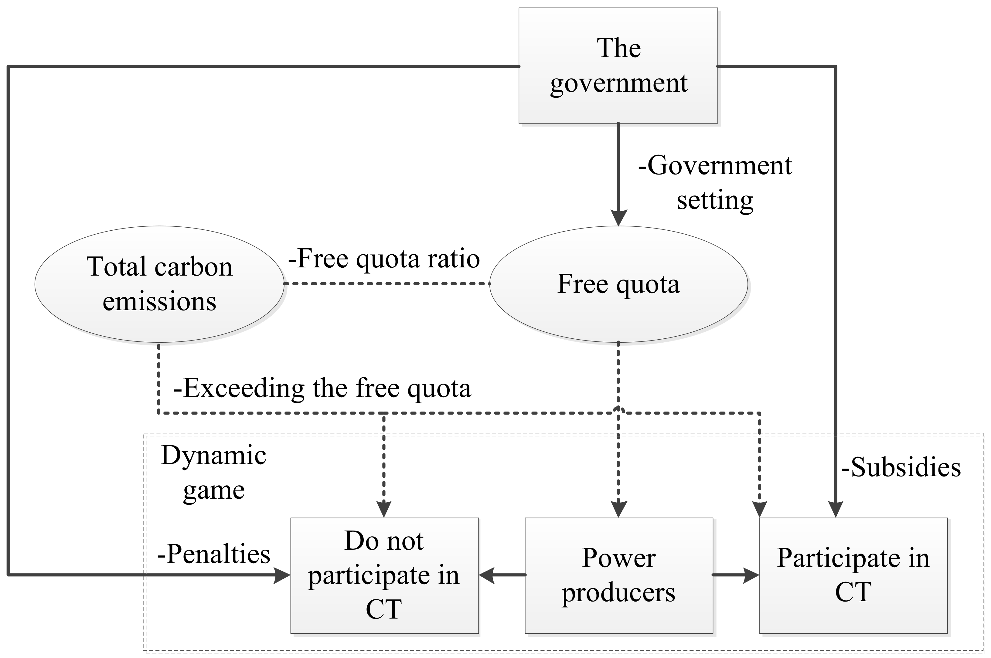
2.1. Theoretical Framing Analysis

It is necessary to explain the CT process and the relationship between the government and power producers under CT before establishing the evolutionary game model, as shown in Figure 1, in which the solid line indicates the behaviors of the government and power producers, and the dotted line indicates the CT amounts. In the CT market, the government acts by setting caps, legislating, motivating participation, introducing trading, and standardizing and supervising the market [4]. The government takes carbon emissions as the total amounts of transactions in the CT market, and accordingly sets a certain percentage of the free quotas, which is the maximum carbon emissions permitted by the power producers. The portion beyond the free quotas requires the power producers to trade at a certain CT price in the market, thereby completing the government’s mandatory carbon emission target for power producers. During the transaction process, the government will give certain incentives to the power producers involved in CT, that is, subsidies [20]. Similarly, the government will impose certain penalties on power producers that do not participate in CT, that is, fines [20]. We regard all the power producers in the market as one game subject in our study, and a dynamic game is formed between the government’s incentive/punishment measures and the decision of the power producers to participate in CT or not.

2.2. Evolutionary Game Model

2.2.1. Game Payment Function

(1) Participants in the game: The two participants in the evolution game of CT are the government and producers, and both of them have bounded rationality.

(2) Participants’ behavior strategies: Power producers have two strategies, which are to participate in CT or not participate in CT. “The strategy of participation in CT (PCT)” includes power producers reducing energy consumption through energy-efficient retrofitting of equipment, thereby reducing carbon emissions. “The strategy of no participation in CT (NPCT)” means that power producers do not take any measures to reduce carbon emissions. At the same time, the government has the duty to supervise the power producers. There are two strategies for the government, that is, supervise (S) and do not supervise (NS) whether the power producers participate in CT [25]. It can be seen as a result of the game between the government and power producers whether a power producer participates in CT or not.

(3) Probabilities of behavioral strategy: In the initial stage of the game between the government and power producers, we suppose that the probability of the government choosing “S” is $x\left(0\le x\le 1\right)$, and then the probability of choosing “NS” is $1-x$. The probability of power producers choosing “PCT” is $y\left(0\le y\le 1\right)$, and then the probability of choosing “NPCT” is $1-y$. The game strategy combination is shown in

Table 1. The game strategy combination of the government and power producers. PCT, participation in carbon trading; NPCT, no participation in carbon trading; S, supervise; NS, do not supervise.

Game Players		Power Producer
		PCT ($\mathit{y}$)	NPCT ($1-\mathit{y}$)
Government	S ($x$)	$\left(x,y\right)$	$\left(x,1-y\right)$
	NS ($1-x$)	$\left(1-x,y\right)$	$\left(1-x,1-y\right)$

.

(4) Game payment functions: The revenue of the game matrix between government and power producers is shown in

Table 2. The revenue of the game matrix between government and power producers.

Game Players		Power Producer
		PCT ($\mathit{y}$)	NPCT ($1-\mathit{y}$)
Government	S ($x$)	$\left({\pi }_1,u_1\right)$	$\left({\pi }_2,u_2\right)$
	NS ($1-x$)	$\left({\pi }_3,u_3\right)$	$\left({\pi }_4,u_4\right)$

. The payment function of each strategy on game players are as follows.

$${\pi }_1=-c_1-r_2=-UCC\times TCE-p_{sub}\times \left(TCE-FQ\right),$$

(1)

$${\pi }_2=-c_1-c_2+P=-UCC\times TCE-UTC\times TCE+f\times \left(TCE-FQ\right),$$

(2)

$${\pi }_3=0,$$

(3)

$${\pi }_4=-c_2=-UTC\times TCE,$$

(4)

$$\begin{array}{l}{u}_1=-c_3+r_1+r_2+r_3=-URC\times TCE\\ +\left(LM{C}_{NCT}-LM{C}_{CT}\right)\times TCE+p_{sub}\times \left(TCE-FQ\right)+p_{CT}\times \left(TCE-FQ\right),\end{array}$$

(5)

$$u_2=-P=-f\times \left(TCE-FQ\right),$$

(6)

$$\begin{array}{l}{u}_3=-c_3+r_1+r_3=-URC\times TCE\\ +\left(LM{C}_{NCT}-LM{C}_{CT}\right)\times TCE+p_{CT}\times \left(TCE-FQ\right),\end{array}$$

(7)

$$u_4=0.$$

(8)

All the variables and their economic meanings are shown in Appendix A. Formula (1) is the government’s revenues when the government supervises and power producers participate in CT. It is the negative value of expenditure costs, including the costs paid by the government during supervision, and subsidies for power producers, which are the product of the unit subsidy and the carbon emissions involved in the CT market. Formula (2) is the government’s revenues when the government supervises and power producers do not participate in CT. The incomes are penalties, which are the product of the unit fine and the carbon emissions should be involved in the CT market, and the expenditures are supervision costs and treatment costs of environmental pollution. Formula (3) which equals 0 is the government’s revenues when the government does not supervise and power producers participate in CT. Formula (4) is the government’s revenues when the government does not supervise and power producers do not participate in CT. It is treatment costs of environmental pollution. Formula (5) is the power producers’ revenues when power producers participate in CT and the government supervises. The incomes include the comprehensive benefits, the subsidies, and the market trading revenues when power producers participate in CT. The expenditures are the costs of energy-saving equipment, where the comprehensive benefits are the reduction of energy consumption costs, which is reflected in the reduction of the long-term marginal cost of carbon emissions. Formula (6) is the power producers’ revenues when power producers do not participate in CT and the government supervises. It is the penalties. Formula (7) is the power producers’ revenues when power producers participate in CT and the government does not supervise. It equals Formula (5) except for subsidies. Formula (8) which equals 0 is the power producers’ revenues when power producers do not participate in CT and the government does not supervise.

2.2.2. Evolutionarily Stable Strategy (ESS)

According to Table 1 and Table 2, the expected return of “S” (${\pi }_x$), the expected return of “NS” (${\pi }_{1-x}$), and average expected return ($\overline{\pi }$) are as follows [26,27,28]:

$${\pi }_x=y\times {\pi }_1+\left(1-y\right)\times {\pi }_2=y\times \left(c_2-r_2-P\right)-c_1-c_2+P,$$

(9)

$${\pi }_{1-x}=y\times {\pi }_3+\left(1-y\right)\times {\pi }_4=y\times c_2-c_2,$$

(10)

$$\overline{\pi }=x\times {\pi }_x+\left(1-x\right)\times {\pi }_{1-x}=-x\times y\times \left(r_2+P\right)+x\times \left(P-c_1\right)+\left(y-1\right)\times c_2.$$

(11)

Thus, the replicated dynamic equation of the government’s evolutionary strategy is:

$$\begin{array}{cc}\hfill F\left(x,y\right)& =\frac{dx}{dt}=x\times \left({\pi }_x-\overline{\pi }\right)=x\times \left(1-x\right)\times \left(P-c_1-y\times r_2-y\times P\right)\hfill \\ & =x\times \left(1-x\right)\times \left[\left(\left(1-y\right)\times f-y\times p_{sub}\right)\times \left(TCE-FQ\right)-UCC\times TCE\right],\hfill \end{array}$$

(12)

Similarly, the expected return of “CT” ($u_y$), the expected return of “NCT” ($u_{1-y}$), and average expected return ($\overline{u}$) are as follows:

$$u_y=x\times u_1+\left(1-x\right)\times u_3=x\times r_2+r_1+r_3-c_3,$$

(13)

$$u_{1-y}=x\times u_2+\left(1-x\right)\times u_4=-x\times P,$$

(14)

$$\overline{u}=y\times u_y+\left(1-y\right)\times u_{1-y}=x\times y\times \left(r_2+P\right)+y\times \left(-c_3+r_1+r_3\right)-x\times P.$$

(15)

Thus, the replicated dynamic equation of power producers’ evolutionary strategy is:

$$\begin{array}{cc}\hfill G\left(x,y\right)& =\frac{dy}{dt}=y\times \left(u_y-\overline{u}\right)=y\times \left(1-y\right)\times \left(r_1+r_3-c_3+x\times r_2+x\times P\right)\hfill \\ & =y\times \left(1-y\right)\times \left[\begin{array}{l}\left(x\times p_{sub}+x\times f+p_{CT}\right)\times \left(TCE-FQ\right)\\ +\left(LM{C}_{NCT}-LM{C}_{CT}-URC\right)\times TCE\end{array}\right].\hfill \end{array}$$

(16)

From Formulas (12) and (16), this can be expressed as a two-dimensional dynamic autonomy system:

$$\{\begin{array}{l}F\left(x,y\right)=\frac{dx}{dt}=x\times \left(1-x\right)\times \left[\left(\left(1-y\right)\times f-y\times p_{sub}\right)\times \left(TCE-FQ\right)-UCC\times TCE\right]\\ G\left(x,y\right)=\frac{dy}{dt}=y\times \left(1-y\right)\times \left[\begin{array}{l}\left(x\times p_{sub}+x\times f+p_{CT}\right)\times \left(TCE-FQ\right)\\ +\left(LM{C}_{NCT}-LM{C}_{CT}-URC\right)\times TCE\end{array}\right].\end{array}$$

(17)

According to the two-dimensional differential theorem, if and only if $0\le \frac{\left(URC-LM{C}_{NCT}+LM{C}_{CT}\right)\times TCE}{\left(p_{sub}+f\right)\times \left(TCE-FQ\right)}-\frac{p_{CT}}{p_{sub}+f}\le 1$ and $0\le \left(f-\frac{UCC\times TCE}{TCE-FQ}\right)/\left(f+p_{sub}\right)\le 1$, the equilibrium points of the system above are $\left(0,0\right)$, $\left(0,1\right)$, $\left(1,0\right)$, $\left(1,1\right)$, and $\left(x^{\ast },y^{\ast }\right)$, where $x^{\ast }=\frac{\left(URC-LM{C}_{NCT}+LM{C}_{CT}\right)\times TCE}{\left(p_{sub}+f\right)\times \left(TCE-FQ\right)}-\frac{p_{CT}}{p_{sub}+f}$, $y^{\ast }=\left(f-\frac{UCC\times TCE}{TCE-FQ}\right)/\left(f+p_{sub}\right)$.

According to the method proposed by Friedman [26,27,28], a system of differential equations describing population dynamics is known, and the stability of the local equilibrium point can be obtained by the analysis of the system’s Jacobian. Thus, the stability of five equilibrium points described above can be analysis according to the Jacobian of Formula (17), which is:

$$\begin{array}{cc}\hfill J& =\left[\begin{array}{cc}\frac{\partial F\left(x,y\right)}{\partial x}& \frac{\partial F\left(x,y\right)}{\partial y}\\ \frac{\partial G\left(x,y\right)}{\partial x}& \frac{\partial G\left(x,y\right)}{\partial y}\end{array}\right]=\left[\begin{array}{cc}\left(1-2x\right)\times \left(P-c_1-y\times P-y\times r_2\right)& x\times \left(x-1\right)\times \left(P+r_2\right)\\ y\times \left(1-y\right)\times \left(P+r_2\right)& \left(1-2y\right)\times \left(r_1+r_3-c_3+x\times r_2+x\times P\right)\end{array}\right]\hfill \\ & =\left[\begin{array}{cc}\left(1-2x\right)\times \left(\left(f-y\times f-y\times p_{sub}\right)\times \left(TCE-FQ\right)-UCC\times TCE\right)& x\times \left(x-1\right)\times \left(f+p_{sub}\right)\times \left(TCE-FQ\right)\\ y\times \left(1-y\right)\times \left(f+p_{sub}\right)\times \left(TCE-FQ\right)& \left(1-2y\right)\times \left(\begin{array}{l}\left(LM{C}_{NCT}-LM{C}_{CT}-URC\right)\times TCE\\ +\left(p_{CT}+x\times psub+x\times f\right)\times \left(TCE-FQ\right)\end{array}\right)\end{array}\right].\hfill \end{array}$$

The local stability of linear differential equations is determined by both determinant ($\det \left(J\right)$) and trace ($tr\left(J\right)$). When the equilibrium point satisfies $\det \left(J\right)=\frac{\partial F\left(x,y\right)}{\partial x}\times \frac{\partial G\left(x,y\right)}{\partial y}-\frac{\partial F\left(x,y\right)}{\partial y}\times \frac{\partial G\left(x,y\right)}{\partial x}>0$ and $tr\left(J\right)=\frac{\partial F\left(x,y\right)}{\partial x}+\frac{\partial G\left(x,y\right)}{\partial y}<0$, this equilibrium point is the ESS. If $\det \left(J\right)<0$, then this equilibrium point is a saddle point. The stability analysis is performed according to the analysis of Jacobian, and the results are shown in

Table 3. The stability analysis of equilibrium points.

Local Equilibrium Point	$\mathbf{det}\left(\mathit{J}\right)$	$\mathit{t}\mathit{r}\left(\mathit{J}\right)$	Stability
$\left(0,0\right)$	-	±	Saddle Point
$\left(0,1\right)$	-	±	Saddle Point
$\left(1,0\right)$	-	±	Saddle Point
$\left(1,1\right)$	-	±	Saddle Point
$\left(x^{\ast },y^{\ast }\right)$	+	0	Center Point

.

It can be seen that the game model has a central point as $\left(x^{\ast },y^{\ast }\right)=\left(\frac{\left(URC-LM{C}_{NCT}+LM{C}_{CT}\right)\times TCE}{\left(p_{sub}+f\right)\times \left(TCE-FQ\right)}-\frac{p_{CT}}{p_{sub}+f},\left(f-\frac{UCC\times TCE}{TCE-FQ}\right)/\left(f+p_{sub}\right)\right)$ and four saddle points as $\left(0,0\right)$, $\left(0,1\right)$, $\left(1,0\right)$, and $\left(1,1\right)$. Therefore, there is no ESS in the evolution of the system, and any slight change may have a huge impact on the system’s behavior [19].

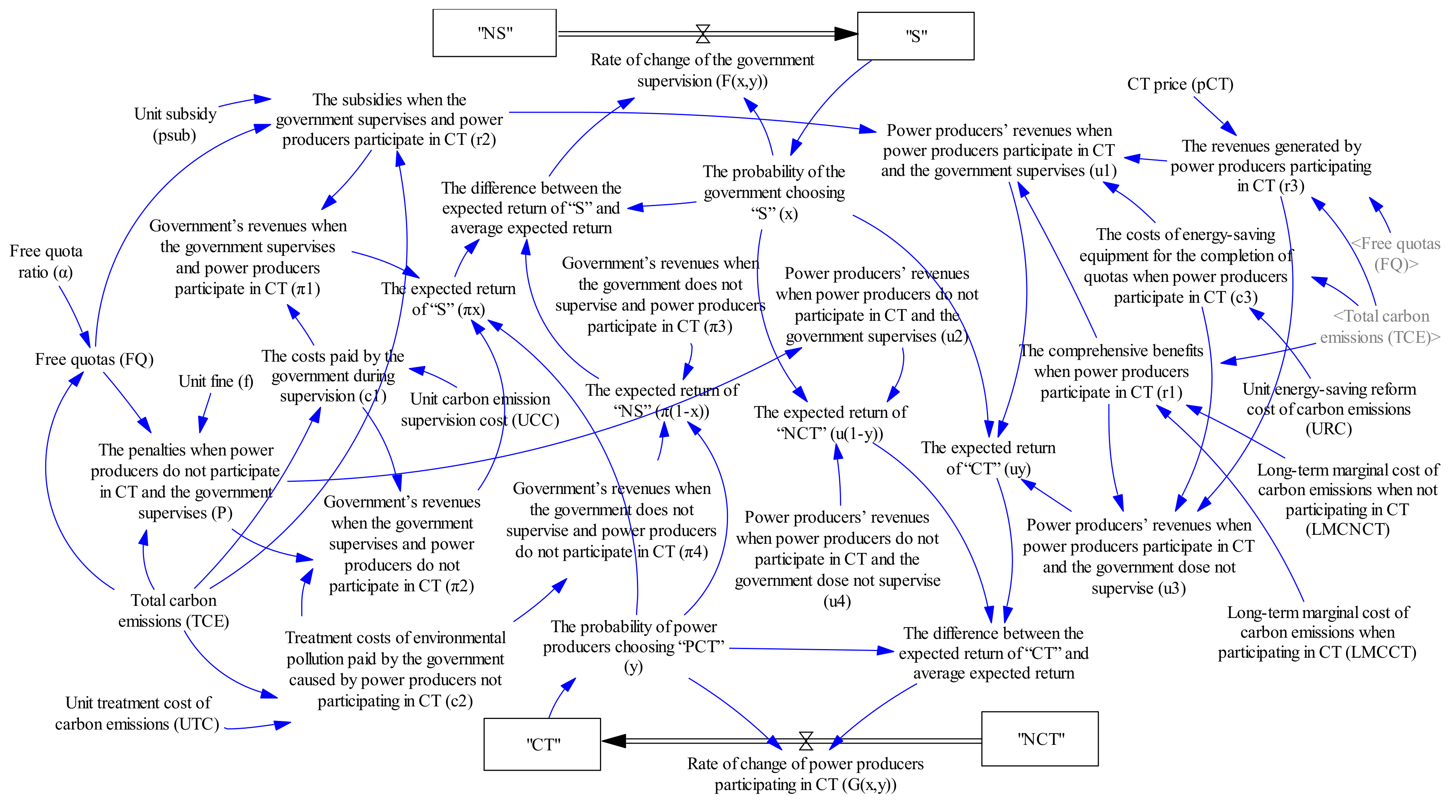
2.3. SD Simulation Model

Based on the analysis of the theoretical framing and evolutionary game model of the relationship between the government and power producers in the CT market, we believe that there are complex nonlinear relationships between the two game players. In order to clearly represent the dynamic evolution of the behavioral strategies of the game players, we establish a stock and flow diagram (SFD) of dynamic game between the government and power producers using Vensim based on the evolutionary game model above, as shown in Figure 2. The SFD is a good tool for modeling the cause and effect relationships between various components of the SD model [29].

There are about 30 functions used to represent the relationship between various factors in the SFD. As most of the functional relationships have been explained in the evolutionary game model, some of other main formulas and important function relationships in the flow chart are listed as follows.

$$x=x_0+{\displaystyle \int F\left(x,y\right)\cdot dt},$$

(18)

$$y=y_0+{\displaystyle \int G\left(x,y\right)\cdot dt}.$$

(19)

Formula (18) is the probability of the government choosing “S”, where, $x_0$ is the initial probability of government supervision. Similarly, Formula (19) is the probability of power producers choosing “PCT”, where, $y_0$ is the initial probability of power producers’ participation of CT.

3. Case Study

3.1. Data

We put the data of China’s CT market into the SD model for simulation. The data are collated according to [20,30,31,32,33,34], and the main sources are related literature, the Chinese Statistical Yearbook, and survey data of China Electricity Council (CEC). We assume that $TCE$ is one unit, and the data of other variables are shown in

Table 4. Data of simulation.

Variables	Data	Unit	Data Resource
Unit carbon emission supervision cost ($UCC$)	37	Yuan/Unit carbon emission	[30,31,32]
Unit treatment cost of carbon emissions ($UTC$)	220	Yuan/Unit carbon emission	[30,31,32]
Unit energy-saving reform cost of carbon emissions ($URC$)	2120	Yuan/Unit carbon emission	[30,31,32]
Long-term marginal cost of carbon emissions when participating in CT ($LM{C}_{CT}$)	3000	Yuan/Unit carbon emission	[33]
Long-term marginal cost of carbon emissions when not participating in CT ($LM{C}_{NCT}$)	5000	Yuan/Unit carbon emission	[33]
Unit subsidy ($p_{sub}$)	100	Yuan/Unit carbon emission	[20,33]
CT price ($p_{CT}$)	120	Yuan/Unit carbon emission	[20,33]
Unit fine ($f$)	150	Yuan/Unit carbon emission	[33,34]
Free quota ratio ($\alpha$)	60%	-	[33,34]

.

3.2. Results Analysis

According to the data, we obtain that $\frac{\left(URC-LM{C}_{NCT}+LM{C}_{CT}\right)\times TCE}{\left(p_{sub}+f\right)\times \left(TCE-FQ\right)}-\frac{p_{CT}}{p_{sub}+f}=0.72$, and $\left(f-\frac{UCC\times TCE}{TCE-FQ}\right)/\left(f+p_{sub}\right)=0.23$, which both meet the prerequisites of evolutionary equilibrium. Since the data in our study is the unit value based on the actual data, the simulation time in the SD model refers to the general time unit rather than a specific setting (such as year and month). In order to study whether the game players will be actively stable to a saddle point, we analyze three scenarios. By comparing the results of our study with that of the related literature [19,25,35,36], we find that the trend of game players’ probabilities and the evolution of the mixed strategy in our study are substantially the same as those in the related literature; this proves that our simulation results are consistent with those of other scholars.

Scenario 1: It is assumed that the initial probability of the government supervision is the equilibrium value of the mixed strategy, and that of power producers participating in CT is random.

Let $x_0=\frac{\left(URC-LM{C}_{NCT}+LM{C}_{CT}\right)\times TCE}{\left(p_{sub}+f\right)\times \left(TCE-FQ\right)}-\frac{p_{CT}}{p_{sub}+f}=0.72$, and the initial probability of power producers’ participation in CT is $y_0=0.2$ and $y_0=0.8$, respectively. The simulation results are shown in Figure 3. We can see that when the initial value of government supervision is set as the equilibrium value of mixed strategy, and the initial value of $y$ is given, the probability of power producers participating in CT fluctuates, and the system will not stabilize to the center point $\left(x^{\ast },y^{\ast }\right)$. In addition, as time and number of games increase, the amplitude of fluctuation of $y$ gradually increases, and it is difficult for the game process to reach a steady state.

Scenario 2: It is assumed that the initial probability of power producers participating in CT is the equilibrium value of the mixed strategy, and that of the government supervision is random.

Let $y_0=\left(f-\frac{UCC\times TCE}{TCE-FQ}\right)/\left(f+p_{sub}\right)=0.23$, the initial probability of the government supervision is $x_0=0.2$ and $x_0=0.8$, respectively. The simulation results are shown in Figure 4. We can see that when the initial value of power producers participating in CT is set as the equilibrium value of mixed strategy, and the initial value of $x$ is given, the probability of government supervision fluctuates, and the system will not stabilize to the center point $\left(x^{\ast },y^{\ast }\right)$. In addition, as time and number of games increase, the amplitude of fluctuation of $x$ gradually increases, and it is difficult for the game process to reach a steady state.

Scenario 3: It is assumed that both of the game players use the same value between 0 and 1 as the initial probability.

Let $x_0=0.5$ and $y_0=0.5$, the simulation results are shown in Figure 5. We can see that the evolution process of the system is a closed-loop line with periodic motion around the starting point, which indicates that the two game players of the government and power producers show a periodic behavior pattern.

4. Discussion

According to the simulation results, we can see that the game system cannot achieve equilibrium under the premise of given variables. The unit subsidy and fine are unchanged in the simulation, that is, the government subsidizes or punishes power producers at the same amount regardless of the probability of power producers participating in CT. The unit subsidy and unit fine are two important variables controlled by the government, which can be changed dynamically according to the degree of actual participation of the power producers in CT. In this section, we will discuss the system’s evolutionary process in the case of dynamic subsidies and dynamic penalties.

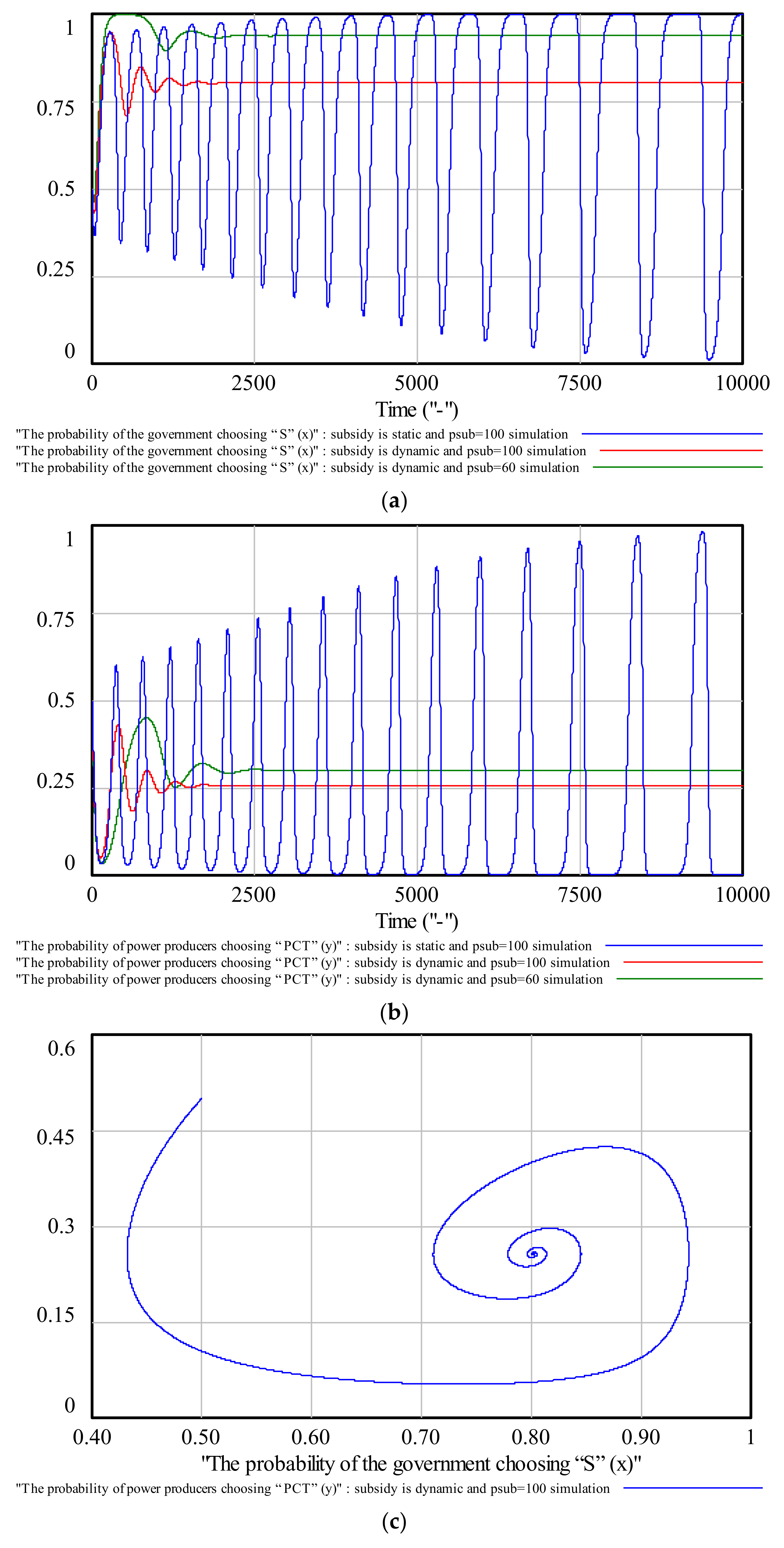
4.1. Dynamic Subsidies

The government adopts a subsidy incentive mechanism to promote the implementation of CT policy by power producers to fulfill emission reduction requirements. In the initial stage of subsidy implementation, when the proportion of power producers participating in CT is low, the government has a strong incentive to motivate power producers participated in CT; thus, the unit subsidy is relatively high. On the contrary, the higher the proportion of power producers participated in CT, the better the implementation of CT policy. Power producers can complete or even exceed the emission reduction targets. At this time, the government’s incentives for encouraging power producers to participate in CT will also reduce, thereby decreasing the unit subsidy. Thus, we assume that the government’s subsidies are inversely proportional to the probability that power producers participate in CT, that is, when power producers participate in CT and the government supervises, the unit subsidy changes from constant $p_{sub}$ to $\left(1-y\right)\times p_{sub}$.

First, we analyze the effect of dynamic subsidies on system’s stability according to replicated dynamic equations and Jacobian stability analysis. $\left(1-y\right)\times p_{sub}$ is substituted into Formula (17), and we obtain that:

$$\{\begin{array}{l}F\left(x,y\right)=\frac{dx}{dt}=x\times \left(1-x\right)\times \left[\left(1-y\right)\times \left(f-y\times p_{sub}\right)\times \left(TCE-FQ\right)-UCC\times TCE\right]\\ G\left(x,y\right)=\frac{dy}{dt}=y\times \left(1-y\right)\times \left[\begin{array}{l}\left(x\times \left(1-y\right)\times p_{sub}+x\times f+p_{CT}\right)\times \left(TCE-FQ\right)\\ +\left(LM{C}_{NCT}-LM{C}_{CT}-URC\right)\times TCE\end{array}\right].\end{array}$$

(20)

We obtain five equilibrium points as $\left(0,0\right)$, $\left(0,1\right)$, $\left(1,0\right)$, $\left(1,1\right)$, and $\left(\frac{\left(URC-LM{C}_{NCT}+LM{C}_{CT}\right)\times TCE}{\left(\left(1-y\right)\times p_{sub}+f\right)\times \left(TCE-FQ\right)}-\frac{p_{CT}}{\left(1-y\right)\times p_{sub}+f},\left(f-\frac{UCC\times TCE}{TCE-FQ}\right)/\left(f+\left(1-y\right)\times p_{sub}\right)\right)$, which satisfies $0<\frac{\left(URC-LM{C}_{NCT}+LM{C}_{CT}\right)\times TCE}{\left(\left(1-y\right)\times p_{sub}+f\right)\times \left(TCE-FQ\right)}-\frac{p_{CT}}{\left(1-y\right)\times p_{sub}+f}<1$ and $0<\left(f-\frac{UCC\times TCE}{TCE-FQ}\right)/\left(f+\left(1-y\right)\times p_{sub}\right)<1$. The Jacobian of the system is:

$$\begin{array}{l}{J}^{\prime }=\left[\begin{array}{cc}\frac{\partial F\left(x,y\right)}{\partial x}& \frac{\partial F\left(x,y\right)}{\partial y}\\ \frac{\partial G\left(x,y\right)}{\partial x}& \frac{\partial G\left(x,y\right)}{\partial y}\end{array}\right]\\ =\left[\begin{array}{cc}\left(1-2x\right)\times \left(\left(1-y\right)\times \left(f-y\times p_{sub}\right)\times \left(TCE-FQ\right)-UCC\times TCE\right)& x\times \left(x-1\right)\times \left(f\times \left(TCE-FQ\right)+\left(1-2y\right)\times p_{sub}\right)\\ y\times {\left(1-y\right)}^2\times \left(\frac{f}{1-y}+p_{sub}\right)\times \left(TCE-FQ\right)& \left(1-2y\right)\times \left(\begin{array}{l}\left(LM{C}_{NCT}-LM{C}_{CT}-URC\right)\times TCE\\ +\left(p_{CT}+x\times f\right)\times \left(TCE-FQ\right)\end{array}\right)+x\times \left(1-y\right)\times \left(1-3y\right)\times p_{sub}\end{array}\right].\end{array}$$

The stability analysis is performed according to the analysis of Jacobian, and the results are shown in

Table 5. The stability analysis of equilibrium points under dynamic subsidies.

Local Equilibrium Point	$\mathbf{det}\left({\mathit{J}}^{\prime }\right)$	$\mathit{t}\mathit{r}\left({\mathit{J}}^{\prime }\right)$	Stability
$\left(0,0\right)$	-	±	Saddle Point
$\left(0,1\right)$	-	±	Saddle Point
$\left(1,0\right)$	-	±	Saddle Point
$\left(1,1\right)$	-	±	Saddle Point
$\left(\begin{array}{l}\frac{\left(URC-LM{C}_{NCT}+LM{C}_{CT}\right)\times TCE}{\left(\left(1-y\right)\times p_{sub}+f\right)\times \left(TCE-FQ\right)}-\frac{p_{CT}}{\left(1-y\right)\times p_{sub}+f}\\ ,\left(f-\frac{UCC\times TCE}{TCE-FQ}\right)/\left(f+\left(1-y\right)\times p_{sub}\right)\end{array}\right)$	+	-	ESS

. It can be seen that the game system with dynamic subsidies has an ESS, which is $\left(\frac{\left(URC-LM{C}_{NCT}+LM{C}_{CT}\right)\times TCE}{\left(\left(1-y\right)\times p_{sub}+f\right)\times \left(TCE-FQ\right)}-\frac{p_{CT}}{\left(1-y\right)\times p_{sub}+f},\left(f-\frac{UCC\times TCE}{TCE-FQ}\right)/\left(f+\left(1-y\right)\times p_{sub}\right)\right)$.

Secondly, we use SD simulation to verify the above conclusion. The simulation results under dynamic subsidies are shown in Figure 6a–c. We can see that, when the subsidy is static and $p_{sub}=100$, $x$ and $y$ oscillate up and down as the time and number of games increase, and the amplitude of fluctuation increases, and it is difficult for the process to reach a steady state. However, when the subsidy is dynamic and $p_{sub}=100$, $x$ and $y$ converge gradually and eventually tend to be stable, and the ESS is $\left(0.8,0.26\right)$. Through SD simulation, we verify that the system has stability under dynamic subsidies.

In addition, we study the changes in probability by changing the value of $p_{sub}$. If the unit subsidy is reduced, namely, when the subsidy is dynamic and $p_{sub}=60$, $x$ and $y$ gradually become stable and improve, that is, reducing unit subsidy can promote the participation of power producers in CT, and at the same time, it can increase the probability of government supervision.

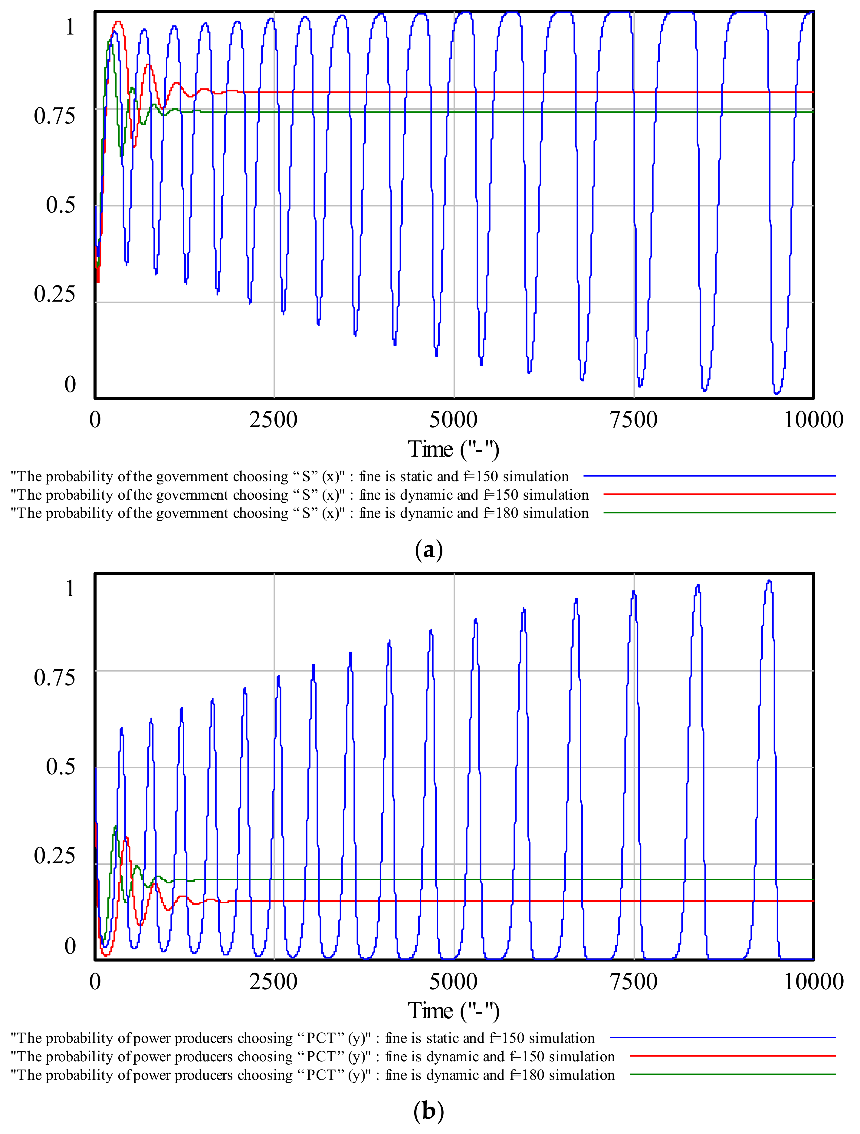
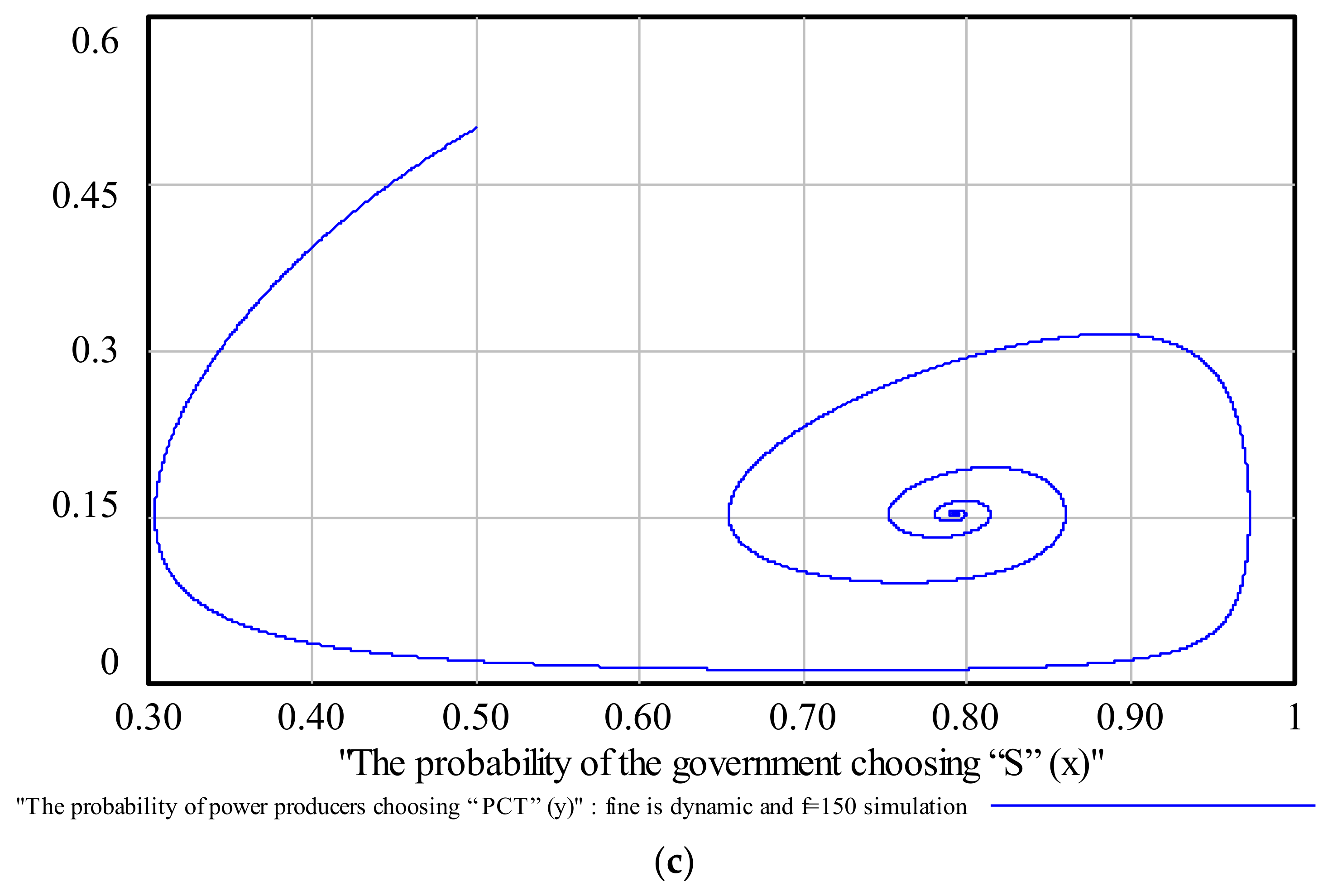
4.2. Dynamic Penalties

Similar to the subsidy mechanism, the government adopts a punitive measure mechanism to promote the implementation of CT policy by power producers from the opposite direction to fulfill emission reduction requirements. In the initial stage of punishment, when the proportion of power producers participating in CT is low, the government has a strong incentive to punish power producers who do not participate in CT; thus, the unit fine is relatively high. On the contrary, the higher the proportion of power producers participated in CT, the better the implementation of CT policy. Power producers can complete or even exceed the emission reduction targets. At this time, the government’s incentives for punishing power producers will also reduce, thereby decreasing the unit fine. Thus, we assume that the government’s penalties are inversely proportional to the probability that power producers participate in CT, that is, when power producers do not participate in CT and the government supervises, the unit fine changes from constant $f$ to $\left(1-y\right)\times f$.

First, we analyze the effect of dynamic penalties on system’s stability according to replicated dynamic equations and Jacobian stability analysis. $\left(1-y\right)\times f$ is substituted into Formula (17), and we obtain that:

$$\{\begin{array}{l}F\left(x,y\right)=\frac{dx}{dt}=x\times \left(1-x\right)\times \left[\left({\left(1-y\right)}^2\times f-y\times p_{sub}\right)\times \left(TCE-FQ\right)-UCC\times TCE\right]\\ G\left(x,y\right)=\frac{dy}{dt}=y\times \left(1-y\right)\times \left[\begin{array}{l}\left(x\times p_{sub}+x\times \left(1-y\right)\times f+p_{CT}\right)\times \left(TCE-FQ\right)\\ +\left(LM{C}_{NCT}-LM{C}_{CT}-URC\right)\times TCE\end{array}\right].\end{array}$$

(21)

We obtain five equilibrium points as $\left(0,0\right)$, $\left(0,1\right)$, $\left(1,0\right)$, $\left(1,1\right)$, and $\left(\frac{\left(URC-LM{C}_{NCT}+LM{C}_{CT}\right)\times TCE}{\left(p_{sub}+\left(1-y\right)\times f\right)\times \left(TCE-FQ\right)}-\frac{p_{CT}}{p_{sub}+\left(1-y\right)\times f},\left(\left(1-y\right)\times f-\frac{UCC\times TCE}{TCE-FQ}\right)/\left(\left(1-y\right)\times f+p_{sub}\right)\right)$, which satisfies $0<\frac{\left(URC-LM{C}_{NCT}+LM{C}_{CT}\right)\times TCE}{\left(p_{sub}+\left(1-y\right)\times f\right)\times \left(TCE-FQ\right)}-\frac{p_{CT}}{p_{sub}+\left(1-y\right)\times f}<1$ and $0<\left(\left(1-y\right)\times f-\frac{UCC\times TCE}{TCE-FQ}\right)/\left(\left(1-y\right)\times f+p_{sub}\right)<1$. The Jacobian of the system is:

$$\begin{array}{l}{J}^{″}=\left[\begin{array}{cc}\frac{\partial F\left(x,y\right)}{\partial x}& \frac{\partial F\left(x,y\right)}{\partial y}\\ \frac{\partial G\left(x,y\right)}{\partial x}& \frac{\partial G\left(x,y\right)}{\partial y}\end{array}\right]\\ =\left[\begin{array}{cc}\left(1-2x\right)\times \left({\left(1-y\right)}^2\times f-y\times p_{sub}\times \left(TCE-FQ\right)-UCC\times TCE\right)& x\times \left(x-1\right)\times \left(2\times \left(1-y\right)\times f-p_{sub}\times \left(TCE-FQ\right)\right)\\ y\times {\left(1-y\right)}^2\times \left(f+\frac{p_{sub}\times \left(TCE-FQ\right)}{1-y}\right)& \left(1-2y\right)\times \left(\begin{array}{l}\left(LM{C}_{NCT}-LM{C}_{CT}-URC\right)\times TCE\\ +\left(p_{CT}+x\times p_{sub}\right)\times \left(TCE-FQ\right)\end{array}\right)-x\times \left(1-y\right)\times \left(1-3y\right)\times f\end{array}\right].\end{array}$$

The stability analysis is performed according to the analysis of the Jacobian, and the results are shown in

Table 6. The stability analysis of equilibrium points under dynamic penalties.

Local Equilibrium Point	$\mathbf{det}\left({\mathit{J}}^{″}\right)$	$\mathit{t}\mathit{r}\left({\mathit{J}}^{″}\right)$	Stability
$\left(0,0\right)$	-	±	Saddle Point
$\left(0,1\right)$	-	±	Saddle Point
$\left(1,0\right)$	-	±	Saddle Point
$\left(1,1\right)$	-	±	Saddle Point
$\left(\begin{array}{l}\frac{\left(URC-LM{C}_{NCT}+LM{C}_{CT}\right)\times TCE}{\left(p_{sub}+\left(1-y\right)\times f\right)\times \left(TCE-FQ\right)}-\frac{p_{CT}}{p_{sub}+\left(1-y\right)\times f}\\ ,\left(\left(1-y\right)\times f-\frac{UCC\times TCE}{TCE-FQ}\right)/\left(\left(1-y\right)\times f+p_{sub}\right)\end{array}\right)$	+	-	ESS

. It can be seen that the game system with dynamic penalties has an ESS, which is $\left(\frac{\left(URC-LM{C}_{NCT}+LM{C}_{CT}\right)\times TCE}{\left(p_{sub}+\left(1-y\right)\times f\right)\times \left(TCE-FQ\right)}-\frac{p_{CT}}{p_{sub}+\left(1-y\right)\times f},\left(\left(1-y\right)\times f-\frac{UCC\times TCE}{TCE-FQ}\right)/\left(\left(1-y\right)\times f+p_{sub}\right)\right)$.

Secondly, we use SD simulation to verify the above conclusion. The simulation results under dynamic penalties are shown in Figure 7a–c. We can see that, when the fine is static and $f=150$, $x$ and $y$ oscillate up and down as the time and number of games increase, and the amplitude of fluctuation increases, and it is difficult for the process to reach a steady state. However, when the fine is dynamic and $f=150$, $x$ and $y$ converge gradually and eventually tend to be stable, and the ESS is $\left(0.79,0.15\right)$. Through SD simulation, we verify that the system has stability under dynamic penalties.

In addition, we study the changes in probability by changing the value of $f$. If the unit fine is increased, namely, when the fine is dynamic and $f=180$, $x$ and $y$ gradually become stable, and $x$ decreases and $y$ increases; that is, raising unit fine can not only promote the participation of power producers in CT, but also reduce the probability of government supervision.

5. Conclusions

Climate warming caused by carbon emissions has become a concern for human beings, and the CT mechanism is one of the effective means to promote carbon emission reduction and achieve green and low-carbon development. It is of great significance to study the evolutionary game process of government and power producers behavioral strategies when implementing CT policy. This paper first constructs the evolutionary game model of the game players, and then uses the SD model to simulate the evolution process of the behavioral strategies. Finally, the stability of the system under the government’s dynamic strategies is discussed. This study provides theoretical guidance and countermeasures for the realization of effective implementation of CT policy and carbon reduction. According to the results of the model, the conclusions of this paper are as follows.

(1)

The evolutionary game model and SD simulation model constructed in this paper can clearly and effectively demonstrate the evolutionary game process of government and power producers’ behavioral strategies under CT, which provide references for scholars to study related issues.

(2)

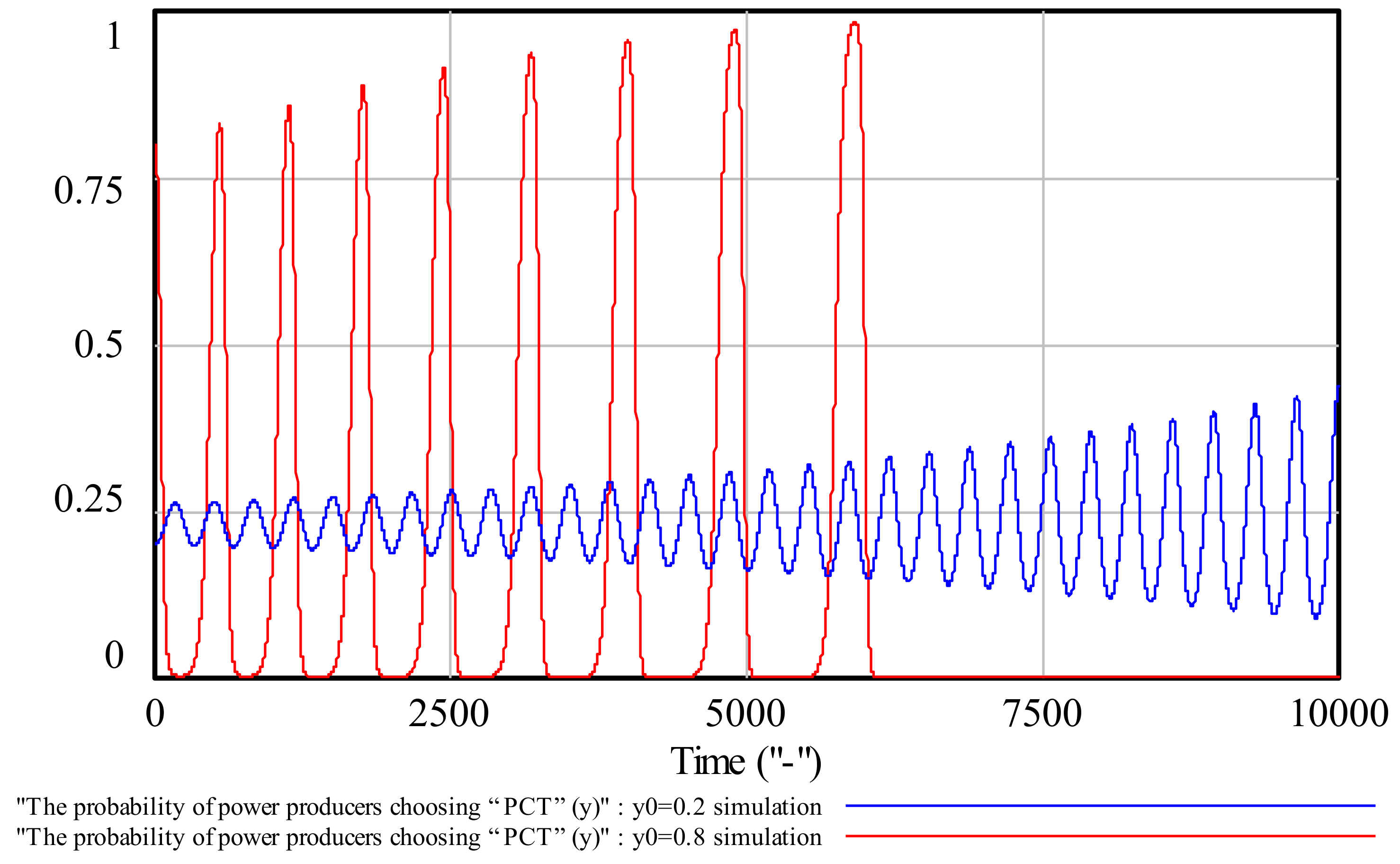
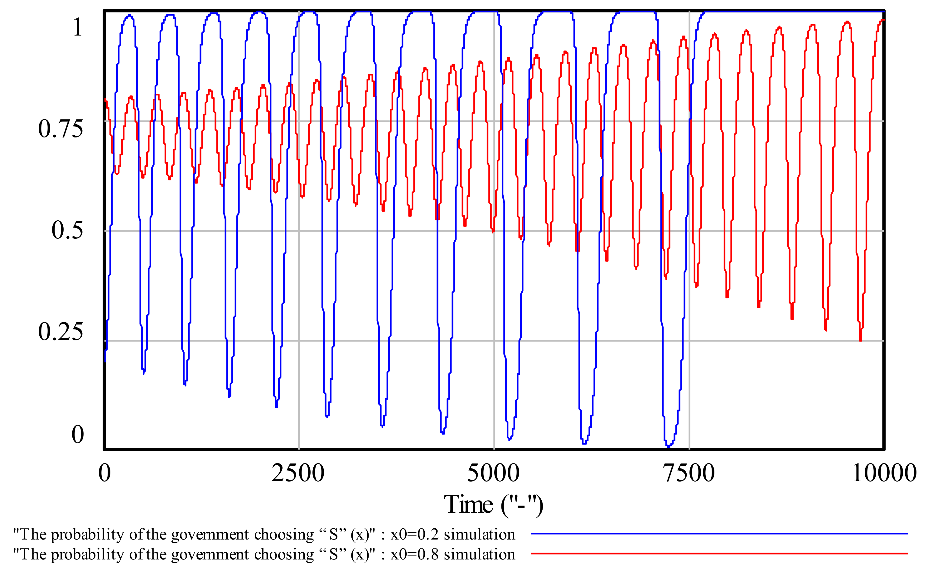
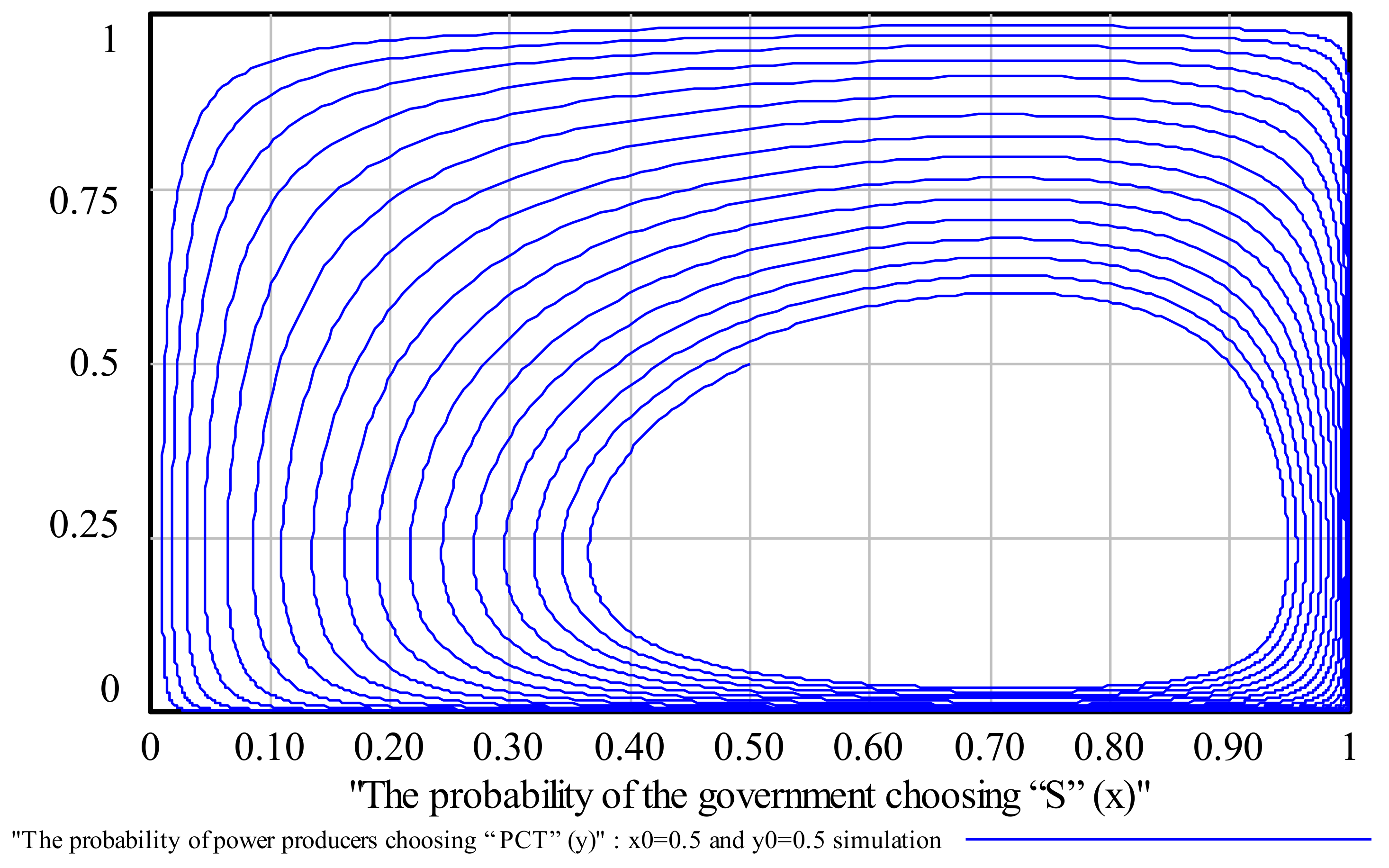
There is a central point and four saddle points in the game system between government and power producers under CT, and there is no ESS. The evolution process of the system is a closed-loop line with periodic motion, which indicates that the two game players of the government and power producers show a periodic behavior pattern.

(3)

The trajectories of game players are spiraling inward and tending to stabilize focus when the government implements dynamic subsidies or penalties. This shows that the probability of government supervision and power producers participating in CT gradually converge with the increase of time, and ultimately stabilizes at the ESS in the mixed strategy, so that the game system can reach equilibrium.

(4)

Reducing the unit subsidy and raising the unit fine can both promote the participation of power producers in CT, but the former increases the probability of government supervision. The purpose of CT implementation is to achieve the optimal allocation of resources through market-oriented means, and the government is only responsible for the basic supervision [37,38]. Thus, it is best to increase the fines when the government makes strategic adjustments, followed by reducing subsidies.

There are still some improvements that could be made in future studies. We believe that the government’s implementation of dynamic subsidies or penalties is conducive to the stability of the system, but in reality, it is difficult for the government to adjust the size of subsidies or fines at any time. Thus, scholars could make an in-depth study of the specific implementation process and mechanisms of dynamic subsidies and penalties in future studies.

References

1. Baidu Net. Paris Agreement. 2016. Available online: https://baike.baidu.com/item/%E5%B7%B4%E9%BB%8E%E5%8D%8F%E5%AE%9A/19138374?fr=aladdin (accessed on 22 April 2016).
2. Central People’s Government of the People’s Republic of China. National Carbon Emissions Trading System Starts. 19 December 2017. Available online: www.gov.cn/xinwen/2017-12/19/content_5248641.htm (accessed on 19 December 2017).
3. Zhao, X.G.; Wu, L.; Li, A. Research on the efficiency of carbon trading market in China. Renew. Sustain. Energy Rev. 2017, 79, 1–8. [Google Scholar] [CrossRef]
4. Zhao, X.G.; Jiang, G.W.; Nie, D.; Chen, H. How to improve the market efficiency of carbon trading: A perspective of China. Renew. Sustain. Energy Rev. 2016, 59, 1229–1245. [Google Scholar]
5. Song, Y.; Liang, D.; Liu, T.; Song, X. How China’s current carbon trading policy affects carbon price? An investigation of the Shanghai Emission Trading Scheme pilot. J. Clean. Prod. 2018, 181, 374–384. [Google Scholar] [CrossRef]
6. Fang, G.; Tian, L.; Liu, M.; Fu, M.; Sun, M. How to optimize the development of carbon trading in China-Enlightenment from evolution rules of the EU carbon price. Appl. Energy 2018, 211, 1039–1049. [Google Scholar]
7. Hu, H.; Xie, N.; Fang, D.; Zhang, X. The role of renewable energy consumption and commercial services trade in carbon dioxide reduction: Evidence from 25 developing countries. Appl. Energy 2018, 211, 1229–1244. [Google Scholar] [CrossRef]
8. Lin, B.; Jia, Z. Impact of quota decline scheme of emission trading in China: A dynamic recursive CGE model. Energy 2018, 149, 190–203. [Google Scholar] [CrossRef]
9. Li, W.; Jia, Z. The impact of emission trading scheme and the ratio of free quota: A dynamic recursive CGE model in China. Appl. Energy 2016, 174, 1–14. [Google Scholar] [CrossRef]
10. Yang, B.; Liu, C.; Gou, Z.; Man, J.; Su, Y. How Will Policies of China’s CO2 ETS Affect its Carbon Price: Evidence from Chinese Pilot Regions. Sustainability 2017, 10, 605. [Google Scholar] [CrossRef]
11. Jiang, H.; Shao, X.; Zhang, X.; Bao, J. A Study of the Allocation of Carbon Emission Permits among the Provinces of China Based on Fairness and Efficiency. Sustainability 2017, 9, 2122. [Google Scholar] [CrossRef]
12. Chen, Y.; Sun, Y.; Wang, C. Influencing Factors of Companies’ Behavior for Mitigation: A Discussion within the Context of Emission Trading Scheme. Sustainability 2018, 10, 414. [Google Scholar] [CrossRef]
13. Song, X.; Lu, Y.; Shuai, C. Optimal Carbon Reduction Strategies in the Building Sector with Emission Trading System. Energy Procedia 2017, 143, 307–312. [Google Scholar] [CrossRef]
14. Zhu, Y.; Li, Y.P.; Huang, G.H. An optimization decision support approach for risk analysis of carbon emission trading in electric power systems. Environ. Model. Softw. 2015, 67, 43–56. [Google Scholar] [CrossRef]
15. Yang, L.; Li, F.; Zhang, X. Chinese companies’ awareness and perceptions of the Emissions Trading Scheme (ETS): Evidence from a national survey in China. Energy Policy 2016, 98, 254–265. [Google Scholar] [CrossRef]
16. Wang, Y.; Chen, W.; Liu, B. Manufacturing/remanufacturing decisions for a capital-constrained manufacturer considering carbon emission cap and trade. J. Clean. Prod. 2017, 14 Pt 3, 1118–1128. [Google Scholar] [CrossRef]
17. Wang, C.; Wang, W.; Huang, R. Supply chain enterprise operations and government carbon tax decisions considering carbon emissions. J. Clean. Prod. 2017, 152, 271–280. [Google Scholar] [CrossRef]
18. Qin, Q.; Liu, Y.; Li, X.; Li, H. A multi-criteria decision analysis model for carbon emission quota allocation in China’s east coastal areas: Efficiency and equity. J. Clean. Prod. 2017, 168, 410–419. [Google Scholar] [CrossRef]
19. Cai, L.R.; Wang, H.W.; Zeng, W. System dynamics model for a mixed-strategy game of environmental pollution. Comput. Sci. 2009, 36, 234–238. [Google Scholar]
20. Zhao, X.; Zhang, Y.; Liang, J.; Li, Y.; Jia, R.; Wang, L. The Sustainable Development of the Economic-Energy-Environment (3E) System under the Carbon Trading (CT) Mechanism: A Chinese Case. Sustainability 2018, 10, 98. [Google Scholar] [CrossRef]
21. Kamarzaman, N.A.; Tan, C.W. A comprehensive review of maximum power point tracking algorithms for photovoltaic systems. Renew. Sustain. Energy Rev. 2014, 37, 585–598. [Google Scholar] [CrossRef]
22. Kim, D.H. A system dynamics model for a mixed-strategy game between police and driver. Syst. Dyn. Rev. 1997, 13, 33–53. [Google Scholar] [CrossRef]
23. Sice, P.; Mosekilde, E.; Moscardini, A.; Lawler, K.; French, I. Using system dynamics to analyse interactions in duopoly competition. Syst. Dyn. Rev. 2000, 16, 113–133. [Google Scholar] [CrossRef]
24. Liu, L.; Feng, C.; Zhang, H.; Zhang, X. Game Analysis and Simulation of the River Basin Sustainable Development Strategy Integrating Water Emission Trading. Sustainability 2015, 7, 4952–4972. [Google Scholar] [CrossRef]
25. Zhu, Q.H.; Wang, Y.L.; Tian, Y.H. Analysis of evolutionary game between local governments and manufacturing enterprises under carbon reduction policies based on system dynamics. Oper. Res. Manag. Sci. 2014, 23, 71–82. [Google Scholar]
26. Friedman, D. Evolutionary games in economics. Econometrica 1991, 59, 637–666. [Google Scholar] [CrossRef]
27. Friedman, D. On economic applications of evolutionary game theory. J. Evol. Econ. 1998, 8, 15–43. [Google Scholar] [CrossRef]
28. Ginits, H. Game Theory Evolving, 2nd ed.; Princeton University Press: Princeton, UK, 2009. [Google Scholar]
29. Zhang, Y.Z.; Zhao, X.G.; Ren, L.Z.; Liang, J.; Liu, P.K. The development of China’s biomass power industry under feed-in tariff and renewable portfolio standard: A system dynamics analysis. Energy 2017, 139, 947–961. [Google Scholar]
30. State Statistical Bureau. China Statistical Yearbook 2016; China Statistics Press: Beijing, China, 2017.
31. State Statistical Bureau. China Energy Statistical Yearbook 2016; China Statistics Press: Beijing, China, 2017.
32. State Statistical Bureau. China Environmental Statistical Yearbook 2016; China Statistics Press: Beijing, China, 2017.
33. China Electricity Council. Statistics. 2017. Available online: www.cec.org.cn/guihuayutongji/tongjxinxi/ (accessed on 1 January 2018).
34. Hang, J.R.; Wang, Z.D.; Tang, L.; Yu, L.A. The Simulation of Carbon Emission Trading System in Beijing-Tianjin-Hebei Region: An Analysis Based on System Dynamics. Chin. J. Manag. Sci. 2016, 24, 1–8. [Google Scholar]
35. Fan, R.; Dong, L. The dynamic analysis and simulation of government subsidy strategies in low-carbon diffusion considering the behavior of heterogeneous agents. Energy Policy 2018, 117, 252–262. [Google Scholar] [CrossRef]
36. Fang, G.; Tian, L.; Fu, M.; Sun, M. Government control or low carbon lifestyle? Analysis and application of a novel selective-constrained energy-saving and emission-reduction dynamic evolution system. Energy Policy 2014, 68, 498–507. [Google Scholar] [CrossRef]
37. Tanpaifang Net. Nature and Institutional Framework of Carbon Trading. 18 November 2015. Available online: www.tanpaifang.com/tanguwen/2015/1118/49044.html (accessed on 18 November 2015).
38. Tengxun Net. Carbon Emissions Trading: Marketization Measures Promote Green and Low Carbon Sustainable Development. 14 March 2017. Available online: http://sh.qq.com/a/20170314/037275.htm (accessed on 14 March 2017).
Figure 1. The carbon trading (CT) process and the relationship between the government and power producers under CT.
Sustainability 10 01150 g001
Figure 2. The stock and flow diagram (SFD) of dynamic game between the government and power producers.
Sustainability 10 01150 g002
Figure 3. The evolution of the probability of power producers participating in CT under different initial values.
Sustainability 10 01150 g003
Figure 4. The evolution of the probability of government supervision under different initial values.
Sustainability 10 01150 g004
Figure 5. The game evolution process of the mixed strategy.
Sustainability 10 01150 g005
Figure 6. The system’s game process under dynamic subsidies.
Sustainability 10 01150 g006
Figure 7. The system’s game process under dynamic penalties.
Sustainability 10 01150 g007aSustainability 10 01150 g007b