The Effects of Land-Use Patterns on Home-Based Tour Complexity and Total Distances Traveled: A Path Analysis

Abstract

This work studies the relationships between the number of complex tours (with one or more intermediate stops) and simple home-based tours, total distances traveled by mode, and land-use patterns both at the residence and at the workplace using path analysis. The model includes commuting distance, car ownership and motorcycle ownership, which are intermediate variables in the relationship between land use, tour complexity and distances traveled by mode. The dataset used here was collected in a region comprising four municipalities located in the north of Portugal that are made up of urban areas, their sprawling suburbs, and surrounding rural hinterland. The results confirm the association between complex tours and higher levels of car use. Land-use patterns significantly affect travelled distances by mode either directly and indirectly via the influence of longer-term decisions like vehicle ownership and commuting distance. The results obtained highlight the role of socioeconomic variables in influencing tour complexity; in particular, households with children, household income, and workers with a college degree tend to do more complex tours. Land-use patterns mediate the effects of tour complexity on the kilometers travelled by different modes. Increasing densities in central areas, and particularly the concentration of jobs, have relevant benefits by reducing car kilometers driven.

1. Introduction

During the 1970s and early 1980s, several researchers recognized the limitations and pitfalls of the trip-based approach as materialized by the 4-step model (e.g., [1,2,3,4,5]). One relevant criticism was that the focus on individual trips ignored the interrelationships between different trips and between trips and activities [6]. From this stemmed the notion that the object of analysis should consist of sequences of patterns of behavior and not individual trips [6]. Therefore, tours, defined as a series of chained trips starting and ending at the same anchor point (usually home or workplace) [7], allow to preserve the consistency of the transport mode, destination and time-of-day throughout the trips undertaken during the day [7,8,9]. Since a tour involves the chaining of trips, both concepts tend to be used interchangeably. Chaining trips, resulting in a smaller number of more complex tours during a day, have been considered as an individual strategy to reduce the total amount of travel, particularly total distances traveled.

Tours are a relevant component of activity-based models (e.g., [10,11]), but compared to other dimensions of travel behavior (e.g., travel mode choice and vehicle distance traveled) tour type and tour complexity have not been the object of much attention in the research relating travel behavior to land-use patterns/urban environment. Theoretically, more dense and diverse urban areas induce trip-chaining as a way to reduce travel distances, but since they could reduce the marginal costs of additional trips that could be included in the chain, the resulting effect might be an increase in the total number of trips [12]. Therefore, denser and more diverse urban areas could actually induce more travel [13,14]. From a sustainability point of view, it is important to know the impact of this in terms of total distances traveled by mode. Changes in lifestyles and more atomized travel patterns have impacts on the levels of trip-chaining and tour complexity. Trip-chaining increased in the past decades, in great part due to changes in the location of specific activities which have moved from in-home to out-home (e.g., stopping for coffee or meals) [15] and to escorting activities (mainly escorting children to school). Trip-chaining leads to more complex travel patterns which, as previous research has highlighted, are correlated with higher levels of car use (e.g., [15,16,17]). This can impact negatively on public transport patronage and result in even more unsustainable travel patterns.

This work aims to study the relationships between the number of complex tours (with one or more intermediate stops) and simple tours, total distances traveled by mode, and land-use patterns both at the residence and at the workplace using path analysis. It draws its inspiration from previous work that studied the relationships between several short- and long-term travel behavior-related dimensions and land-use patterns both at the residence and employment locations while accounting for self-selection [18]; and work that studied the effects of land-use patterns on choice of tour type [14]. The model also includes commuting distance, car ownership and motorcycle ownership, which are intermediate variables in the relationships between land use, tour complexity and distances traveled by mode. The dataset used here was collected in a region comprising four municipalities (Barcelos, Braga, Guimarães and Vila Nova de Famalicão), with a combined total population of 594,841 inhabitants. These four municipalities are located in the north of Portugal and comprise both urban areas (the four cities which are the seats of the four municipalities) their sprawling suburbs and surrounding rural hinterland. The rural hinterland is characterized by a pattern of small villages and hamlets intersected by small farms. From a travel diary with a sample of 4433 surveys, collected in 2012, a subsample of 1153 workers who live and work inside these four municipalities is used here.

This paper makes several contributions to the literature. It develops a modeling framework that incorporates explicitly the endogenous relationships in the chain of decisions relating residence and workplace characteristics, commuting distance, car and motorcycle ownership, tour complexity and travel distances by mode. To the best of my knowledge, this is the first time that trip-chaining behavior has been integrated in such a comprehensive framework. Secondly, it incorporates motorcycle ownership which is generally overlooked in travel-behavior studies. Thirdly, it studies these relationships in a region which includes both urban and rural areas where most studies on trip-chaining and tour frequency and complexity have focused mainly on urban and metropolitan areas.

The remainder of this work is organized as follows: a literature review focusing on the relationships between tour complexity and trip-chaining and land-use patterns is offered. The following section describes the model global framework, the modeling method used here, and a description of the case study and the data used. Section 3 presents and discusses the model results. The paper ends with the conclusions and a brief discussion of policy implications.

Literature Review

Increasing tour complexity by chaining trips enables individuals to link secondary and primary activities [19]. Besides consolidating trips, trip-chaining might also induce new travel [13]. Empirical research on the relationships relating land-use patterns with trip-chaining, tour frequency and tour complexity have so far produced mixed results. Several studies focused on different components of tours and trip-chaining and also on different tour purposes. In some cases, the focus has been on commuting tours, but there is also research on non-work tours. The dimensions studied included tour frequency, tour complexity and tour transport mode choice. Land-use variables included in these studies varied significantly, both in scope and in location: home-related land-use variables, work-related land-use variables and tour main destination characteristics. Only a limited number of studies have considered self-selection effects [13,14,20,21,22] and even fewer have studied tours in the context of other travel-related decisions, e.g., car ownership [20,23,24] and mode choice [17,20,25].

The effects of land-use characteristics on tour complexity and frequency are mixed. Density has been found to reduce tour complexity [21,26,27], increase it [28,29,30] or be neutral [31]. Lee [32] argues that living in more walkable neighborhoods increases the likelihood of performing simple tours. Mixing urban activities could increase trip-chaining [12,33,34,35] and, therefore, increase tour complexity. The effects of accessibility are also mixed. Neighborhood accessibility together with regional accessibility was found to decrease tour complexity [36,37]. On the contrary, other authors [26,38], argue that greater public transport accessibility increases trip-chaining. Noland and Thomas [27] claim that higher accessibility leads to more travel and Cao et al. [13] that it increases tour complexity. Other authors found out that land-use characteristics at the workplace have stronger effects on tour complexity [22,28,39] than the ones in the vicinity of the residence. Land-use patterns at the workplace could have different effects than similar patterns at the residence area. Higher density, mixed uses and transit accessibility at the workplace location lead to more complex tours [26,30]. Retail density and accessibility of destinations can also increase tour complexity [40,41]. The effects of land-use patterns on tour frequency are also mixed. Living in zones with higher accessibility was found not to influence shopping tours’ frequency [40], while other studies argue that higher density and walkability in the residence area increases tour frequency [26,32].

Another characteristic that land use could influence is tour travel mode choice [31,32,39,42]. In general, these results tend to corroborate the reported effects of land-use patterns/urban environment on transport mode choice (e.g., [14,34,35,43,44,45]). Transit access, mixed and dense land uses, and higher levels of walkability increase the probability of using transit and non-motorized modes [32,39,42]. Increasing tour complexity diminishes the likelihood of using non-motorized modes [32] and public transport [16,46]. More complex tours are associated with higher levels of car use [19,20,24,47,48]. The use of public transport in more complex trip chains is dependent on the adequacy of transit supply and the concentration of activities around its stops [47,49,50]. Tour complexity creates relevant challenges to public transport operators [17,51]. Besides land-use patterns, socioeconomic characteristics also influence tour characteristics. Several socioeconomic characteristics have been found to be associated with increased tour complexity. The presence of children in the household is associated with more complex tours [25,29,30,46,47,52]. Household income also correlates positively with tour complexity [29,46,52], although Chen and Akar [30] argue otherwise. Women tend to have more complex tour patterns [25,29,52]. Having a college degree increases tour complexity [25]. Members of larger households [30,46] and older people [25,30] engage in simpler tours.

2. Materials and Methods

2.1. Model Framework

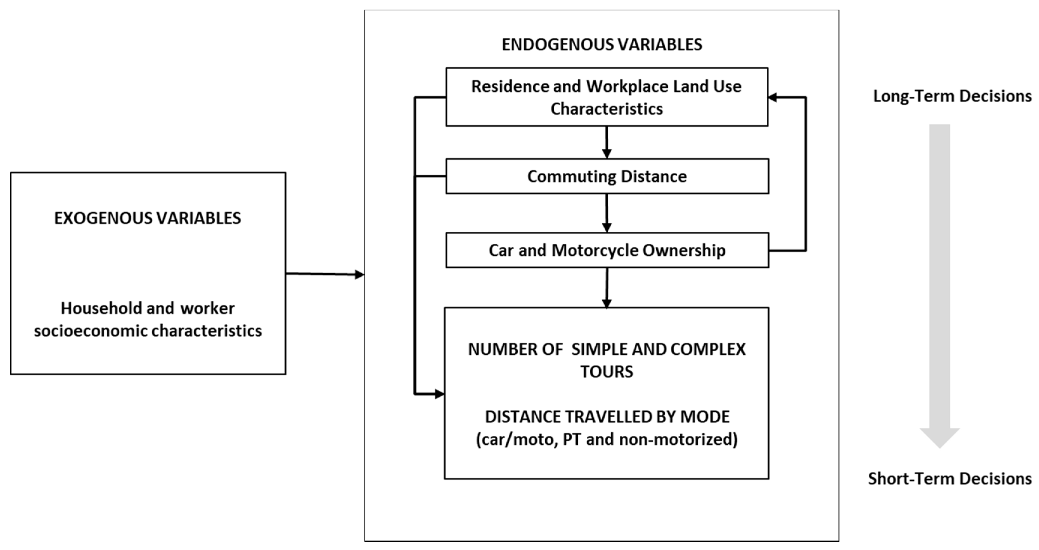
The model global structure (Figure 1) was devised explicitly to introduce the frequency of simple and complex tours (tours with at least one intermediate stop) within a framework that considers both longer-term decisions related to location patterns, spatial self-selection [42], commuting distance, car and motorcycle ownership and shorter-term decisions related to daily distances travelled by mode. Apart from the socioeconomic variables, all the other variables are endogenous to the model. Thus, the model incorporates self-selection effects due to needs (e.g., household composition, presence of children), abilities and restrictions (e.g., income) [45,53,54] that could be correlated with socioeconomic characteristics. Globally the effects go from long-term decisions to short-term ones, but feedback effects [55], in which car ownership affects location patterns, are also considered. Although some studies focused on several of the referred relationships, like self-selection [13,14,20,21,22], car ownership [20,23,24], and the relationship between tour complexity and mode choice [17,20,25], none of the reviewed studies has included all the relationships modeled here.

2.2. Model Methodology

The modelling method used here is path analysis (also known as simultaneous equation modelling). Path analysis is a special case of structural equation modelling (SEM) [56,57] when all variables included in the different model equations are observed. The general equation for this method is:

Y = By + Γx + ζ

(1)

where,

• B is the matrix containing the coefficients for the equations relating the endogenous variables;
• y is the vector of the endogenous variables;
• Γ is the matrix containing the coefficients for the equations relating the exogenous with the endogenous variables;
• x is the vector of the exogenous variables;
• ζ is the vector of the residuals from the structural relationships between y and x.

The fact that these methods are able to model simultaneously several endogenous variables and handle direct and indirect relationships makes them particularly adequate to study complex relationships between travel behavior and urban environment. The model results include direct (equivalent to regression coefficients), indirect (sum of the effects mediated by other variables) and total effects (sum of the total and indirect effects). Direct effects give a clear image about the model structure, but the total effects allow for a better interpretation, since due to possible contradictory direct and indirect effects, model interpretation based only in the direct effects might lead to misleading conclusions. The estimation method used here is Weighted Least Squares (WLS). This method was developed to deal with binary, ordered and censored variables [58] as in the present case. Since WLS uses correlation matrices, the resulting coefficients are standardized, facilitating a direct comparison between the magnitudes of the different effects.

2.3. Case Study and Data

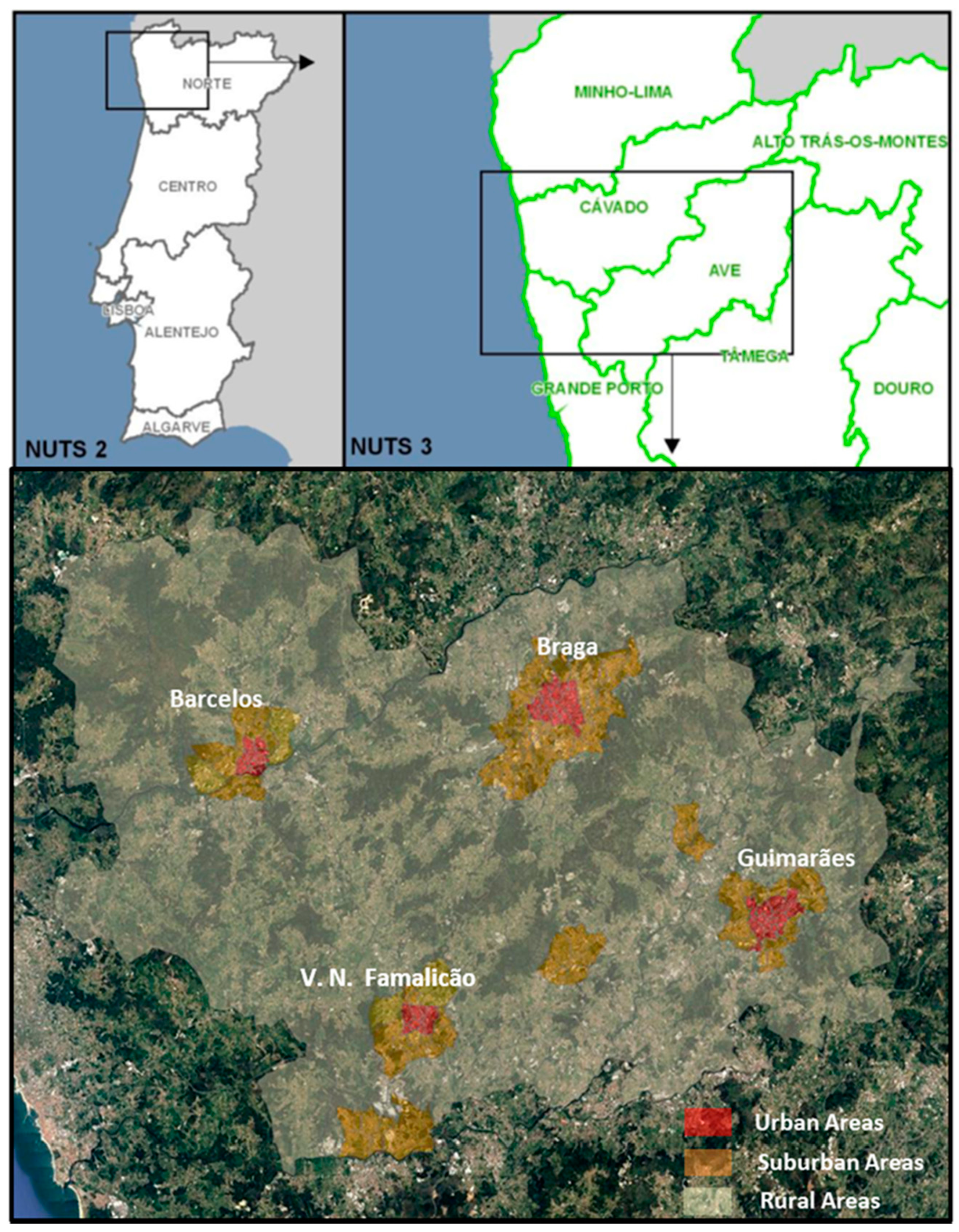
The data used here is a subsample from a mobility survey implemented in four neighboring municipalities (Barcelos, Braga, Guimarães and Vila Nova de Famalicão), belonging to the NUTS 3 (Nomenclature of territorial units for statistics) of Cávado (Braga and Barcelos) and Ave (Guimarães and Vila Nova de Famalicão), in the north of Portugal (Figure 2). The data was collected, between May and June of 2012, for an Integrated Mobility Plan developed for these 4 municipalities [59]. The survey was implemented by the consultants who developed the mobility plan, using stratified random sampling. Six different strata differentiated by age (15–17-year-olds; 18–65-year-olds; and older than 65) and gender were used. Households were contacted, and one of each household members was randomly selected and asked to fill a travel diary for the last weekday. The socioeconomic characteristics of all the individuals in the household where collected, as well as the characteristics of the vehicles owned by its members. The subsample included only households where the interviewed member was a worker with a workplace inside of the study area, so that the land-use characteristics of the employment location could also be measured. The 4 referred municipalities, with a total population of 593,841 inhabitants and occupying 1005 km², form a homogeneous sub-region with similar occupation patterns and economic specialization. Besides the cities which are the seats of each of the 4 municipalities’ the study area is characterized by dispersed occupations where small villages and hamlets are intersected by small farms and more recently by small industrial units. Although its population density (590 inhab/km²) is five times larger than mainland Portugal (114 inhab/km²) the percentage of urban population (people residing in urban agglomerations with 2000 or more inhabitants) is smaller (51.0% against 63.1% for mainland Portugal). Within the study area, different zones were classified as urban (4% of the study area), suburban (9% of the study area), and rural (the remaining 87% of the study area) based on population densities. The urban areas correspond also to the seats of the four municipalities and are surrounded by less dense suburban areas. The zones classified as urban are on average denser, more urbanized, with a higher proportion of multi-family buildings, and have a denser road network (

Table 1. Land-use indicators (mean values).

Zones	Global Density (Residents, Workers and Students) (People/ha)	% of Urban Residents	% of Urban Space	% of Multi-Family Buildings	Road Network Density (km/ha)
Urban	51.62	62%	33%	38%	0.023
Suburban	21.13	66%	20%	22%	0.006
Rural	5.25	22%	3%	7%	0.003
Global	8.46	28%	6%	10%	0.004

).

Most of the travel is internal to the study area and the commuting relationships between the 4 municipalities are relatively balanced. Although there are some specific locations in the road network with congestion problems, the global average saturation level is 23% [59]. The study area is served both by rail and road public transport services, although the former mostly serve external trips. Internal public transport services are provided by 18 different operators, resulting in a heterogeneous spatial and temporal coverage, being that the more exurban and rural areas experience the worst levels of service. This atomization of operators exacerbates the perceived problems of physical and tariff integration.

Table 2. Sample characteristics and descriptive statistics.

Variables	Global Sample (4433 Observations)		Workers Subsample (1153 Observations)
	Mean	Coefficient of Variation	Mean	Coefficient of Variation
Age	41.509	0.430	38.183	0.266
% man	48.2%		50.7%
% university degree	23.6%		27.8%
Household size	3.279	0.375	3.486	0.328
Average age of the household	42.589	0.363	36.850	0.315
Number of household workers	1.566	0.714	2.192	0.415
% of households with children	20.5%		30.9%
Household income (€/month)	1348.748	0.790	1614.918	0.704
Number of cars in the household	1.598	0.616	1.807	0.513
Number of motorcycles in the household	0.117	3.232	0.129	3.173
Simple commuting tours (without intermediate stops)/individual	0.446	1.439	0.973	0.728
Complex commuting tours (with intermediate stops)/individual	0.054	4.254	0.112	2.867
Simple tours for other purpose (without intermediate stops)/individual	0.347	1.745	0.241	2.077
Complex tours for other purpose (with intermediate stops)/individual	0.075	3.689	0.108	3.107
Km travelled by private vehicles/individual	15.130	3.336	17.505	1.833
Km travelled by public transport/individual	3.070	6.506	1.054	6.058
Km travelled by non-motorized/individual	0.515	3.378	0.584	3.308
Implied modal shares (distances traveled)
% private vehicles	80.8%		91.4%
% public transport	16.4%		5.5%
% non-motorized	2.8%		3.0%
Implied tour shares
% simple commuting tours	48.4%		67.9%
% complex commuting tours	5.8%		7.8%
% simple tours other purpose	37.7%		16.8%
% complex tours other purpose	8.1%		7.5%

presents the descriptive statistics from both the global survey sample (representative of the global population older than 14 years old) and the workers’ subsample. As expected, the workers’ subsample presents some differences: workers are younger, more educated belonging to wealthier and bigger households. They are also more mobile, chain more trips, leading to a higher proportion of more complex tours, rely more on private vehicles and much less on public transport.

The socioeconomic variables included in the model were selected based on the literature review adjusted to take into account potential problems of collinearity. They comprised age, gender, household size, household average age, possession of a college degree, number of household workers, presence of children (10 years old and younger) in the household and household monthly income.

The study area was divided into 142 transport analysis zones (TAZs) and several land-use variables were collected for each TAZ. Urban form exhibits a multidimensionality that is difficult to capture [60] with interconnections between different land-use variables [20,61]. One way to solve this issue is to group land-use variables into global indexes [61]. Principal components factor analysis was used to reduce the collected land-use variables in 5 factors capturing the multidimensional characteristics of urban space both at the residence and workplace TAZs.

Table 3. Rotated land-use factor matrix loadings (KMO = 0.867, % of explained variance = 77.43%).

Land Use Factor	Land Use Variable	Loadings
Living in a dense central urban area	Residence zone is an urban center (1 = yes)	0.846
	Road network density at the residence zone	0.758
	% of multi-family buildings at the residence zone	0.855
	Global density at the residence zone	0.882
	% of urban residents at the residence zone	0.774
	% of urban space at the residence zone	0.927
Working in a dense central urban area	Workplace zone is an urban center (1 = yes)	0.834
	Road network density at the workplace zone	0.685
	% of multi-family buildings at the workplace zone	0.767
	Global density at the workplace zone	0.839
	% of urban residents at the workplace zone	0.716
	% of urban space at the workplace zone	0.891
Living in an accessible area	Public transport accessibility at the residence zone	0.792
	Car accessibility at the residence zone	0.807
	Travel time to the nearest freeway intersection at the residence zone	−0.778
	Travel time to the nearest railway station at the residence zone	−0.825
Working in an accessible area	Public transport accessibility at the workplace zone	0.749
	Car accessibility at the workplace zone	0.766
	Travel time to the nearest freeway intersection at the workplace zone	−0.804
	Travel time to the nearest railway station at the workplace zone	−0.699
Entropy	Entropy at the residence zone	0.774
	Entropy at the workplace zone	0.614

presents the obtained factors, their defining variables and respective loadings.

These variables include a binary variable classifying the TAZ as being part of an urban center; a global density (considering the sum of residents, workers and students); the road network density (excluding freeways); the percentage of residents living in urban areas inside the TAZ; the percentage of urban space in the TAZ; the percentage of multifamily buildings; public transport and car gravity-based accessibility indicators; travel time to the nearest railway station and freeway intersection; and an entropy index [45], measuring the diversity of different categories of urban space (residential, industrial, infrastructures and construction spaces).

The first four factors present a clear distinction between resident and workplace TAZs. The first and second factors present high loadings in several variables associated with more urbanized, denser and central areas; therefore, they were named, respectively, “Living in a dense and central” area and “Working in a dense and central area”. The third and fourth factors are mainly associated with higher levels of accessibility both at the residence and workplace TAZs; therefore, they were named “Living in an accessible area” and “Working in an accessible area”. The fifth factor is associated with higher land-use diversity both at the residence and workplace TAZ, and was named “Entropy”.

3. Results and Discussion

The model presents a very good fit. The chi-square statistic is 96.708 (with 127 degrees of freedom and a p-value of 0.979), resulting in a ratio between the chi-square and the degrees of freedom, smaller than 1, which is indicative of a good fit [62,63]. The Goodness of Fit Index (GFI) is 0.997 and, in addition, both Bayesian-fit indicators, the Akaike Information Criterion (AIC) and the consistent Akaike Information Criterion (CAIC), present values smaller than the saturated model and independence model, indicating that the estimated model is superior to both. The results are presented in

Table 4. Standardized direct and total effects due to exogenous variables.

Endogenous Variables	Effects	Exogenous Variables
		Age	Gender (1 = Man)	HH Size	HH Average Age	University Degree (1 = Yes)	HH # Employees	HH Children (1 = Yes)	HH Income
Km travelled car/motorcycle	direct	-	0.142	-	-	-	-	-	0.481
	total	-	0.142	0.000	−0.022	−0.085	0.000	0.032	0.563
Km travelled Public Transport	direct	-	−0.151	-	-	-	-	-	-
	total	-	−0.170	−0.054	0.031	−0.093	−0.034	−0.023	−0.024
Km travelled non-motorized	direct	-	-	-	0.102	-	-	-	-
	total	0.019	−0.048	−0.083	0.134	−0.045	−0.062	0.100	−0.028
# Complex tours	direct	-	-	-	-	0.162	-	0.162	-
	total	-	0.000	0.001	−0.107	0.205	0.000	0.161	0.015
# Simple tours	direct	-	-	-	0.127	−0.081	-	-	-
	total	-	0.000	0.008	0.125	−0.103	0.002	−0.004	−0.001
# Cars	direct	-	0.149	0.395	−0.237	0.244	0.257	−0.481	0.127
	total	-	0.151	0.395	−0.240	0.241	0.257	−0.481	0.127
# Motos	direct	−0.210	0.206	-	0.207	-	0.095	-	-
	total	−0.210	0.194	0.015	0.198	−0.056	0.098	−0.007	0.025
Ln Commuting distance	direct	-	-	-	-	0.135	-	-	-
	total	-	0.014	0.033	−0.008	0.081	0.008	−0.016	0.021
Living in a dense central urban area	direct	-	-	−0.096	-	0.235	-	-	-
	total	-	−0.024	−0.158	0.037	0.197	−0.040	0.075	−0.020
Working in a dense central urban area	direct	-	-	-	-	0.338	-	-	−0.211
	total	-	-	-	-	0.338	-	-	−0.211
Living in an accessible area	direct	-	−0.046	-	0.056	0.080	-	-	-
	total	-	−0.046	-	0.056	0.080	-	-	-
Working in an accessible area	direct	-	0.078	-	-	0.109	-	-	-
	total	-	0.078	-	-	0.109	-	-	-
Entropy	direct	-	0.082	-	-	-	-	-	−0.062
	total	-	0.082	-	-	-	-	-	−0.062

Note: coefficients significant at 95% presented in bold; HH stands for Household; Ln stands for natural logarithm; # stands for number.

, which presents the direct and total effects due to the exogenous (socioeconomic) variables, and in

Table 5. Standardized direct and total effects due to endogenous variables.

Endogenous Variables	Effects	Endogenous Variables
		# Complex Tours	# Simple Tours	# Cars	# Motos	Ln Commuting Distance	Living in a Dense Central Urban Area	Working in a Dense Central Urban Area	Living in an Accessible Area	Working in an Accessible Area	Entropy
Km travelled car/motorcycle	direct	0.201	-	-	-	-	-	−0.374	-	-	-
	total	0.201	−0.170	0.000	-	−0.001	−0.001	−0.388	0.000	0.000	-
Km travelled Public Transport	direct	−0.531	−0.451	−0.127	-	-	-	-	-	-	-
	total	−0.531	−0.002	−0.131	-	0.046	0.025	0.034	0.006	0.006	-
Km travelled non-motorized	direct	-	-	−0.206	−0.088	-	-	-	-	-	-
	total	-	-	−0.207	−0.088	−0.010	0.008	0.007	0.018	0.014	0.007
# Complex tours	direct	-	−0.845	-	-	−0.087	−0.065	−0.071	-	-	-
	total	-	−0.845	0.001	-	−0.005	−0.003	−0.071	0.000	−0.001	-
# Simple tours	direct	-	-	-	-	−0.096	−0.072	-	-	-	-
	total	-	-	0.008	-	−0.096	−0.052	0.007	0.000	−0.012	-
# Cars	direct	-	-	-	-	-	-	-	−0.043	-	-
	total	-	-	-	-	-	-	-	−0.043	-	-
# Motorcycles	direct	-	-	-	-	0.112	−0.069	−0.076	−0.101	−0.168	−0.084
	total	-	-	0.014	-	0.112	−0.092	−0.084	−0.102	−0.154	−0.084
Ln Commuting distance	direct	-	-	-	-	-	−0.208	−0.078	-	0.120	-
	total	-	-	0.033	-	-	−0.208	−0.078	−0.001	0.120	-
Living in a dense central urban area	direct	-	-	−0.156	-	-	-	-	-	-	-
	total	-	-	−0.156	-	-	-	-	0.007	-	-

Note: coefficients significant at 95% presented in bold. # stands for number.

, presenting the direct and total effects between endogenous variables.

3.1. Effects Due to Exogenous Variables

The effects of socioeconomic variables on travel are in accordance with previous findings on the literature, income has a very strong effect on private vehicle miles driven followed by gender. Being a man increases the likelihood of travelling more by private vehicle and much less by public transport and non-motorized modes. The higher percentage of adult men with a driver’s license (89% of adult men own a driver’s license compared with 65% of adult women) contributes to explain these effects and the higher use of public transport and non-motorized modes by women. Wealthier, more educated workers, with children [19,25,26,27,29,46,52] and belonging to younger households are more likely to engage in more complex tours. These results highlight the behavioral effects resulting from the presence of children in the household and related activities of escorting them (mainly to school activities) in conditioning their parents travel patterns. Although escorting trips only represent around 4% of all trips in this region, they are almost exclusively made by car (98%). Escorting trips made by workers are almost exclusively (around 88%) from households with children or teenagers, being that 62% of the escorting trips are made in households with children. Between 2001 and 2011, the share of students commuting to school as car passengers almost doubled (from 21% to 41%). The share of car-driver commuters also rose substantially, from 43% to 64%. These parallel increases highlight the interrelationship between commuting by car and escorting students to school. They are aligned with similar children-commuting patterns observed in other European countries [64,65]. Car-oriented lifestyles, distances to school and perceptions about safety contributed to increase the share of car use in children’s trips [64,66,67,68], thus impacting adult travel patterns. The positive total effects of the presence of children in the number of kilometers driven by car are passed via their effects on the number of complex tours on car travel.

The effects of gender on the number of tours are passed via the effects of gender on commuting distance and car and motorcycle ownership, resulting in non-significant total effects of gender. The effects of having a college degree are negative on travelled distances by all modes. This might be a result of the location patterns of more educated people, which tend to live and work in more urban and accessible environments, therefore contributing to reduce their amount of travel. The total effects of education levels on the distance travelled by non-motorized modes are about half the total effects on car and public transport traveled distances, an indication of their preferences for the former. The negative total effects on public transport have a higher magnitude than the effects on private vehicle travel, hinting that more educated workers do not see it as a viable alternative to the car.

The results also show the existence of self-selection effects due to individual and household characteristics and preferences captured by socioeconomic variables. Workers with a university degree have a higher likelihood of working and living in central and denser areas as well as in more accessible ones, indicating both preferences for more urban environments, in accordance with recent studies (e.g., [69]), and reflecting the concentration of jobs in the service sector in central and accessible areas, which are more aligned with the skills of these workers. Also, by living and working in central areas they are able to reduce commuting distances, as evidenced by Table 4, an attractive feature of urban areas to middle-class and knowledge workers [70,71].

The effects on commuting distance are in accordance with previous findings (e.g., [16]); workers with higher income, with a university degree and also men have longer commutes. Nevertheless, the indirect effects from the location patterns of more educated workers reduce substantially the total effects on commuting distance. The model shows some evidence that motorcycles are representative of a first wave of motorization, and that motorcycle owners are more concentrated in less dense, central and accessible areas (see Table 5) as Yamamoto [72] has found. It can be seen that differences exist between households who own more motorcycles when compared with those who own more cars. Income has a much stronger effect on car ownership and having a university degree has a contrary effect on car and motorcycle ownership. Also, households with more cars tend to be older and larger than those who own motorcycles.

3.2. Effects between Endogenous Variables

Making more complex tours increases the number of kilometers travelled by private vehicles and strongly reduces the kilometers travelled by public transport, indicating that people with more complex patterns of mobility do not see public transport as an alternative. The total effects of simple tours reduce the kilometers travelled by private vehicles but their total effect on public transport is non-significant. These results confirm previous research [16,17], which found an association between complex tours and higher levels of car use. They are in accordance with Ye at al. [17] who pointed out that the direction of influence goes from tour type choice to mode choice. These results also highlight the specific characteristics of the study area, in which public transport supply is mainly based on buses which do not serve adequately the more exurban areas and has a very low urban form efficiency related to access to public transport services [73]. Land-use patterns affect travel distances by mode significantly, but their magnitude is much smaller in promoting the use of both public transport and non-motorized modes than in reducing the number of kilometers driven by car/motorcycle (working in a dense central urban area is the strongest determinant of the number of kilometers driven). These results, together with the fact that the levels of congestion within the studied area are low [59], suggest that the effects of land use on private vehicle use consist mainly in reducing travel distances (and making them more compatible with non-motorized modes), rather than transferring demand to public transport by influencing relative travel costs.

Performing more simple tours implies a reduction in the number of complex tours. All the other total effects on complex tours, with the exception of working in a dense and central area, are non-significant, meaning that different indirect effects coming from commuting distance, number of simple tours and land-use patterns tend to annul each other. This corroborates findings that point to the stronger effects of work locations on tour complexity [22,28,39], but it is contrary to the positive effects of denser areas on tour complexity [26,30]. The effect of working in central and dense areas is related to the effect this land-use factor has on commuting distance (reducing it). Longer commutes might be associated with more complex tours, as some research has shown [15]. Here, commuting distance negatively influences the number of simple tours, thereby capturing this effect. Commuting is the result of location patterns of both workplace and residence; not accounting for the influence of land-use patterns on commuting distance might inflate the effects of the former on the number of complex tours. Besides commuting distance, the number of simple tours is mainly negatively influenced by living in dense and central urban areas. These results suggest that commuting to more exurban areas induces more complex tours in order to save time and reduce total travel distances. In these exurban areas, schools and other urban functions are also dispersed (increasing travel distances) and have lower accessibility by public transport. These spatial patterns are also an incentive for parents to escort their children to school [66,67], thus contributing to more complex tours. These results point to the difficulties in reducing the levels of private vehicle use in low-density sprawled areas where public transport supply has to cope with low levels of demand and, therefore, reduce frequency to balance operating costs with revenues, thus limiting its attractiveness. Comparing the standardized total effects due to the endogenous variables (Table 5) with those from the exogenous variables (Table 4), it can be concluded that socioeconomic factors are stronger determinants of tour complexity than land-use patterns. The role of land use seems to be more relevant in influencing kilometers driven by mode.

Self-selection effects resulting from individual preferences, given by the effects of car ownership in reducing the likelihood of living in more central and urban areas, evidence the important role of car ownership as an intermediate variable between location patterns and travel behavior. This effect has also emerged in several studies using the same modeling approach and a similar structure supporting the robustness of the model [14,74]. Car ownership is only influenced by living in an accessible area, showing the effects of land use on car ownership. But this relatively weak effect could be partly due to two aspects. The first is the strong increase of motorization rates in Portugal during the last two decades, motivated both by economic growth and easy access to credit. The second is the combined result of public transport levels of service, the absence of strong parking regulations’ enforcement, and the percentage of housing with dedicated parking, which reduce the effects of density on the costs of car ownership and use. Living in more remote, urban and less-accessible areas increases the likelihood of owning more motorcycles, corroborating the findings of Yamamoto [72], reinforcing the perception that rural populations tend to own more motorcycles than urban ones, a sign of the differences in the motorization patterns of both rural and urban households. Living and working in central and dense urban areas reduces commuting distance. By contrast, working in accessible areas will increase commuting distance clearly, showing the polarizing effects of more accessible areas.

4. Conclusions

A path-analysis model was built to study the relationships between the frequency of simple and complex tours and distances travelled by mode while incorporating within the same framework, vehicle ownership, commuting distance and land-use patterns. The results confirm the association between complex tours and higher levels of car use. Land-use patterns significantly affect travelled distances by mode both directly and indirectly, via the influence of longer-term decisions like vehicle ownership, a strong determinant of mode choice, and commuting distance. The results obtained also highlight the role of socioeconomic variables in tour complexity, in particular households with children, household income, and workers with a college degree. They were found to increase the frequency of complex tours strongly. The conditions imposed by the presence of children in the household (e.g., escorting them to school and other activities) lead to more complex tours, not compatible with the current public transport system, and result in higher levels of car use and a reduction of transit patronage. These socioeconomic variables, which can capture the effects of workers’ needs and preferences, are stronger determinants of tour complexity than land-use characteristics. But land-use patterns can also mediate the effects of tour complexity on the kilometers travelled by different modes. A clear example of this effect is the case of workers with a university degree. Although they have a higher propensity to engage in more complex tours, their location patterns induce a negative effect on the kilometers driven by car.

In this low-density, sprawled region, the effects of land use reside mainly in affecting travel distances, making some of them (in the denser areas) more compatible with non-motorized modes. The effects on public transport use although positive have a small magnitude. Global low densities and reduced congestion levels prevent public transport being a competitive alternative to the car. The low transit patronage contributes to an increase in the operational deficits of public transport operators and, consequently, prevents any increase in services, particularly in the less dense and more outlying areas, reinforcing their residents’ dependence on private transport (car/motorcycles). All of these effects contribute to a challenging policy context where the low levels of children’s independent mobility [68] patterns coupled with a sprawled region contribute to unsustainable mobility patterns. But the model results also show that increasing densities in central areas, and particularly the concentration of jobs in these central areas, has relevant benefits by reducing car kilometers driven.

References

- Fried, M.; Havens, J.; Thall, M. Travel Behavior—A Synthesized Theory; Laboratory of Psychosocial Studies, Boston College: Chestnut Hill, MA, USA, 1977; p. 145. [Google Scholar]
- Häagerstraand, T. What about people in regional science? Pap. Reg. Sci. 1970, 24, 7–24. [Google Scholar] [CrossRef]
- Jones, P.M.; Dix, M.C.; Clarke, M.I.; Heggie, I.G. Understanding Travel Behaviour; Gower: Aldershot, UK, 1983; ISBN 0-566-00606-5. [Google Scholar]
- Chapin, F.S. Free time activities and quality of urban life. J. Am. Inst. Plan. 1971, 37, 411–417. [Google Scholar] [CrossRef]
- Heggie, I.G. Putting behaviour into behavioural models of travel choice. J. Oper. Res. Soc. 1978, 29, 541–550. [Google Scholar] [CrossRef]
- McNally, M.; Rindt, C. The activity-based approach. In Handbook of Transport Modelling, 2nd ed.; Hensher, D.A., Button, K.J., Eds.; Pergamon: Oxford, UK, 2007; pp. 55–73. ISBN 978-0-08-045376-7. [Google Scholar]
- Davidson, W.; Donnelly, R.; Vovsha, P.; Freedman, J.; Ruegg, S.; Hicks, J.; Castiglione, J.; Picado, R. Synthesis of first practices and operational research approaches in activity-based travel demand modeling. Transp. Res. Part Policy Pract. 2007, 41, 464–488. [Google Scholar] [CrossRef]
- Gunn, H. The Netherlands national model: A review of seven years of application. Int. Trans. Oper. Res. 1994, 1, 125–133. [Google Scholar] [CrossRef]
- Bowman, J.L.; Ben-Akiva, M.E. Activity-based disaggregate travel demand model system with activity schedules. Transp. Res. Part Policy Pract. 2000, 35, 1–28. [Google Scholar] [CrossRef]
- Kitamura, R. An Evaluation of Activity-Based Travel Analysis; Kluwer Academic Publishers: Dordrecht, The Netherlands, 1988; Volume 15, ISBN 0049-4488. [Google Scholar]
- Shiftan, Y. The use of activity-based modeling to analyze the effect of land-use policies on travel behavior. Ann. Reg. Sci. 2008, 42, 79–97. [Google Scholar] [CrossRef]
- Crane, R. On form versus function: Will the new urbanism reduce traffic, or increase it? J. Plan. Educ. Res. 1996, 15, 117–126. [Google Scholar] [CrossRef]
- Cao, X.; Mokhtarian, P.L.; Handy, S.L. Differentiating the influence of accessibility, attitudes, and demographics on stop participation and frequency during the evening commute. Environ. Plan. B Plan. Des. 2008, 35, 431–442. [Google Scholar] [CrossRef]
- de Abreu e Silva, J.; Sottile, E.; Cherchi, E. Effects of land use patterns on tour type choice application. TRR J. Transp. Res. Board 2014, 2453, 100–108. [Google Scholar] [CrossRef]
- McGuckin, N.; Zmud, J.; Nakamoto, Y. Trip-chaining trends in the United States: Understanding travel behavior for policy making. Transp. Res. Rec. J. Transp. Res. Board 2005, 1917, 199–204. [Google Scholar] [CrossRef]
- Ho, C.; Mulley, C. Intra-household Interactions in tour-based mode choice: The role of social, temporal, spatial and resource constraints. Transp. Policy 2015, 38, 52–63. [Google Scholar] [CrossRef]
- Ye, X.; Pendyala, R.M.; Gottardi, G. An exploration of the relationship between mode choice and complexity of trip chaining patterns. Transp. Res. Part B Methodol. 2007, 41, 96–113. [Google Scholar] [CrossRef]
- e Silva, J.; Golob, T.; Goulias, K. Effects of land use characteristics on residence and employment location and travel behavior of urban adult workers. Transp. Res. Rec. J. Transp. Res. Board 2006, 1977, 121–131. [Google Scholar] [CrossRef]
- Primerano, F.; Taylor, M.A.P.; Pitaksringkarn, L.; Tisato, P. Defining and Understanding Trip Chaining Behaviour; Springer: New York, NY, USA, 2008; Volume 35, pp. 55–72. ISBN 1111600791348. [Google Scholar]
- Pinjari, A.R.; Pendyala, R.M.; Bhat, C.R.; Waddell, P.A. Modeling the choice continuum: An integrated model of residential location, auto ownership, bicycle ownership, and commute tour mode choice decisions. Transportation 2011, 38, 933–958. [Google Scholar] [CrossRef]
- La Paix, L.; Bierlaire, M.; Cherchi, E.; Monzón, A. How urban environment affects travel behaviour: Integrated choice and latent variable model for travel schedules. In Choice Modelling: The State of the Art and the State of Practice: Selected Papers from the Second International Choice Modelling Conference; Hess, S., Daly, A., Eds.; Edward Elgar Publishing: Cheltenham, UK, 2013; pp. 211–228. ISBN 978-1-78100-726-6. [Google Scholar]
- van Acker, V.; Witlox, F. Commuting trips within tours: How is commuting related to land use? Transportation 2011, 38, 465–486. [Google Scholar] [CrossRef]
- Ding, C.; Wang, D.; Liu, C.; Zhang, Y.; Yang, J. Exploring the influence of built environment on travel mode choice considering the mediating effects of car ownership and travel distance. Transp. Res. Part Policy Pract. 2017, 100, 65–80. [Google Scholar] [CrossRef]
- Konduri, K.C.; Ye, X.; Sana, B.; Pendyala, R.M. A joint tour-based model of vehicle type choice and tour length. Transp. Res. Rec. J. Transp. Res. Board 2011, 28–37. [Google Scholar] [CrossRef]
- Islam, M.T.; Habib, K.M.N. Unraveling the relationship between trip chaining and mode choice: Evidence from a multi-week travel diary. Transp. Plan. Technol. 2012, 35, 409–426. [Google Scholar] [CrossRef]
- Ma, J.; Mitchell, G.; Heppenstall, A. Daily travel behaviour in Beijing, China: An analysis of workers’ trip chains, and the role of socio-demographics and urban form. Habitat Int. 2014, 43, 263–273. [Google Scholar] [CrossRef]
- Noland, R.B.; Thomas, J.V. Multivariate analysis of trip-chaining behavior. Environ. Plan. B Plan. Des. 2007, 34, 953–970. [Google Scholar] [CrossRef]
- Maat, K.; Timmermans, H. Influence of land use on tour complexity: A Dutch case. Transp. Res. Rec. J. Transp. Res. Board 2007, 1977, 234–241. [Google Scholar] [CrossRef]
- Antipova, A.; Wang, F. Land use impacts on trip-chaining propensity for workers and nonworkers in Baton Rouge, Louisiana. Ann. GIS 2010, 16, 141–154. [Google Scholar] [CrossRef]
- Chen, Y.; Akar, G. Using trip chaining and joint travel as mediating variables to explore the relationships among travel behavior, socio-demographics, and urban form. J. Transp. Land Use 2017, 10, 573–588. [Google Scholar] [CrossRef]
- Portoghese, A.; Spissu, E.; Bhat, C.R.; Eluru, N.; Meloni, I. A copula-based joint model of commute mode choice and number of non-work stops during the commute. Int. J. Transp. Econ. 2011, 38, 337–362. [Google Scholar]
- Lee, J. Impact of neighborhood walkability on trip generation and trip chaining: Case of Los Angeles. J. Urban Plan. Dev. 2016, 142, 05015013. [Google Scholar] [CrossRef]
- Crane, R. Cars and drivers in the new suburbs: Linking access to travel in neotraditional planning. J. Am. Plann. Assoc. 1996, 62, 51–65. [Google Scholar] [CrossRef]
- Van Wee, B. Land use and transport: Research and policy challenges. J. Transp. Geogr. 2002, 10, 259–271. [Google Scholar] [CrossRef]
- Naess, P. Urban structures and travel behaviour. Experiences from empirical research in Norway and Denmark. Land Use Travel Behav. 2000, 3, 1–24. [Google Scholar]
- Krizek, K.J. Residential relocation and changes in urban travel: Does neighborhood-scale urban form matter? J. Am. Plann. Assoc. 2003, 69, 265–281. [Google Scholar] [CrossRef]
- Krizek, K.J. Neighborhood services, trip purpose, and tour-based travel. Transportation 2003, 30, 387–410. [Google Scholar] [CrossRef]
- Greenwald, M.J.; McNally, M.G. Land-use influences on trip-chaining in Portland, Oregon. Proc. Inst. Civ. Eng. Urban Des. Plan. 2008, 161, 61–73. [Google Scholar] [CrossRef]
- Frank, L.; Bradley, M.; Kavage, S.; Chapman, J.; Lawton, T.K. Urban form, travel time, and cost relationships with tour complexity and mode choice. Transportation 2008, 35, 37–54. [Google Scholar] [CrossRef]
- Limanond, T.; Niemeier, D.A. Effect of land use on decisions of shopping tour generation: A case study of three traditional neighborhoods in WA. Transportation 2004, 31, 153–181. [Google Scholar] [CrossRef]
- Srinivasan, S. Quantifying spatial characteristics for travel behavior models. Transp. Res. Rec. 2001, 1777, 1–15. [Google Scholar] [CrossRef]
- Srinivasan, S. Quantifying spatial characteristics of cities. Urban Stud. 2002, 39, 2005–2028. [Google Scholar] [CrossRef]
- de Abreu e Silva, J.; Martinez, L.; Goulias, K. Using a multi equation model to unravel the influence of land use patterns on travel behavior of workers in Lisbon. Transp. Lett. 2012, 4, 193–209. [Google Scholar] [CrossRef]
- Aditjandra, P.T. The impact of urban development patterns on travel behaviour: Lessons learned from a British metropolitan region using macro-analysis and micro-analysis in addressing the sustainability agenda. Res. Transp. Bus. Manag. 2013, 7, 69–80. [Google Scholar] [CrossRef]
- de Abreu e Silva, J. Spatial self-selection in land-use–travel behavior interactions: Accounting simultaneously for attitudes and socioeconomic characteristics. J. Transp. Land Use 2014, 7, 63–84. [Google Scholar] [CrossRef]
- Hensher, D.A.; Reyes, A.J. Trip chaining as a barrier to the propensity to use public transport. Transportation 2000, 27, 341–361. [Google Scholar] [CrossRef]
- Currie, G.; Delbosc, A. Exploring the trip chaining behaviour of public transport users in Melbourne. Transp. Policy 2011, 18, 204–210. [Google Scholar] [CrossRef]
- Wu, Z.; Ye, X. Joint modeling analysis of trip-chaining behavior on round-trip commute in the context of Xiamen, China. Transp. Res. Rec. J. Transp. Res. Board 2008, 2076, 62–69. [Google Scholar] [CrossRef]
- Concas, S.; DeSalvo, J. The effect of density and trip-chaining on the interaction between urban form and transit demand. J. Public Transp. 2014, 17, 16–38. [Google Scholar] [CrossRef]
- Aditjandra, P.T.; Cao, X.; Mulley, C. Exploring changes in public transport use and walking following residential relocation: A British case study. J. Transp. Land Use 2015. [Google Scholar] [CrossRef]
- Vande Walle, S.; Steenberghen, T. Space and time related determinants of public transport use in trip chains. Transp. Res. Part Policy Pract. 2006, 40, 151–162. [Google Scholar] [CrossRef]
- Lee, Y.; Hickman, M.; Washington, S. Household type and structure, time-use pattern, and trip-chaining behavior. Transp. Res. Part Policy Pract. 2007, 41, 1004–1020. [Google Scholar] [CrossRef]
- Cao, X.; Mokhtarian, P.L.; Handy, S.L. Examining the Impacts of Residential Self-Selection on Travel Behaviour: A Focus on Empirical Findings; Routledge Taylor and Francis Group: London, UK, 2009; Volume 29, ISBN 0144164080253. [Google Scholar]
- Cao, X. Residential self-selection in the relationships between the built environment and travel behavior: Introduction to the special issue. J. Transp. Land Use 2014, 7, 1–3. [Google Scholar] [CrossRef]
- Domencich, T.; McFadden, D.L. Urban Travel Demand: A Behavioral Analysis; North-Holland Publishing Co.: Amsterdam, The Netherlands, 1975; ISBN 0-444-10830-0. [Google Scholar]
- Bollen, K.A. Structural Equations with Latent Variables; John Wiley and Sons: Hoboken, NJ, USA, 1989; ISBN 0-471-011711-1. [Google Scholar]
- Kaplan, D. Structural Equation Modeling: Foundations and Extensions; SAGE: Thousand Oaks, CA, USA, 2000. [Google Scholar]
- Golob, T.F. Structural equation modeling for travel behavior research. Transp. Res. Part B Methodol. 2003, 37, 1–25. [Google Scholar] [CrossRef]
- Atkins Way2Go Consultores Associados. Estudo de Mobilidade Integrada—Barcelos, Braga, Famalicão, Guimarães, Tomo 2.1 Relatório de Caracterização; Way2Go Consultores Associados: Lisbon, Portugal, 2013. [Google Scholar]
- Krizek, K.J. Planning, household travel, and household lifestyles. In Transportation Systems Planning, Methods and Applications; New Directions in Civil Engineering; CRC Press: Boca Raton, FL, USA, 2002; p. 456. ISBN 978-1-4200-4228-3. [Google Scholar]
- Stead, D.; Marshall, S. The relationships between urban form and travel patterns: An international review and evaluation. Eur. J. Transp. Infrastruct. Res. 2001, 1, 113–141. [Google Scholar]
- Schermelleh-Engel, K.; Moosbrugger, H.; Müller, H. Evaluating the fit of structural equation models: Tests of significance and descriptive goodness-of-fit measures. Methods Psychol. Res. Online 2003, 8, 23–74. [Google Scholar] [CrossRef]
- Joreskog, K.G.; Sorbom, D. LISREL 8: Structural equation modeling with the SIMPLIS command language. Sci. Softw. Int. 1993, XVI, 202. [Google Scholar]
- Mackett, R.L. Children’s travel behaviour and its health implications. Transp. Policy 2013, 26, 66–72. [Google Scholar] [CrossRef]
- Kyttä, M.; Hirvonen, J.; Rudner, J.; Pirjola, I.; Laatikainen, T. The last free-range children? Children’s independent mobility in Finland in the 1990s and 2010s. J. Transp. Geogr. 2015, 47, 1–12. [Google Scholar] [CrossRef]
- Fyhri, A.; Hjorthol, R. Children’s independent mobility to school, friends and leisure activities. J. Transp. Geogr. 2009, 17, 377–384. [Google Scholar] [CrossRef]
- Fyhri, A.; Hjorthol, R.; Mackett, R.L.; Fotel, T.N.; Kyttä, M. Children’s active travel and independent mobility in four countries: Development, social contributing trends and measures. Transp. Policy 2011, 18, 703–710. [Google Scholar] [CrossRef]
- Lopes, F.; Cordovil, R.; Neto, C. Children’s independent mobility in Portugal: Effects of urbanization degree and motorized modes of travel. J. Transp. Geogr. 2014, 41, 210–219. [Google Scholar] [CrossRef]
- Frenkel, A.; Bendit, E.; Kaplan, S. Residential location choice of knowledge-workers: The role of amenities, workplace and lifestyle. Cities 2013, 35, 33–41. [Google Scholar] [CrossRef]
- Karsten, L. Housing as a way of life: Towards an understanding of middle-class families’ preference for an urban residential location. Hous. Stud. 2007, 22, 83–98. [Google Scholar] [CrossRef]
- Lawton, P.; Murphy, E.; Redmond, D. Residential preferences of the “creative class”? Cities 2013, 31, 47–56. [Google Scholar] [CrossRef]
- Yamamoto, T. Comparative analysis of household car, motorcycle and bicycle ownership between Osaka metropolitan area, Japan and Kuala Lumpur, Malaysia. Transportation 2009, 36, 351–366. [Google Scholar] [CrossRef]
- Jacobs-Crisioni, C.; Kompil, M.; Baranzelli, C.; Lavalle, C. Indicators of Urban Form and Sustainable Urban Transport; Joint Research Centre, European Commission: Ispra, Italy, 2015; pp. 1–36. [Google Scholar]
- de Abreu e Silva, J.; Morency, C.; Goulias, K.G. Using structural equations modeling to unravel the influence of land use patterns on travel behavior of workers in Montreal. Transp. Res. Part Policy Pract. 2012, 46, 1252–1264. [Google Scholar] [CrossRef]
Figure 1.
Model global structure.
Figure 2.
The study area.