Optimal Placement and Sizing of PV-STATCOM in Power Systems Using Empirical Data and Adaptive Particle Swarm Optimization

Department of Electrical and Electronic Engineering, Eastern Mediterranean University, Gazimagusa, 99628 Mersin 10, Turkey
Sustainability 2018, 10(3), 727; https://doi.org/10.3390/su10030727
Submission received: 12 February 2018
/
Revised: 1 March 2018
/
Accepted: 4 March 2018
/
Published: 7 March 2018
(This article belongs to the Collection Power System and Sustainability)
Abstract
:Solar energy is a source of free, clean energy which avoids the destructive effects on the environment that have long been caused by power generation. Solar energy technology rivals fossil fuels, and its development has increased recently. Photovoltaic (PV) solar farms can only produce active power during the day, while at night, they are completely idle. At the same time, though, active power should be supported by reactive power. Reactive power compensation in power systems improves power quality and stability. The use during the night of a PV solar farm inverter as a static synchronous compensator (or PV-STATCOM device) has recently been proposed which can improve system performance and increase the utility of a PV solar farm. In this paper, a method for optimal PV-STATCOM placement and sizing is proposed using empirical data. Considering the objectives of power loss and cost minimization as well as voltage improvement, two sub-problems of placement and sizing, respectively, are solved by a power loss index and adaptive particle swarm optimization (APSO). Test results show that APSO not only performs better in finding optimal solutions but also converges faster compared with bee colony optimization (BCO) and lightening search algorithm (LSA). Installation of a PV solar farm, STATCOM, and PV-STATCOM in a system are each evaluated in terms of efficiency and cost.
1. Introduction
In power systems, active power should be supported by reactive power for power system requirements [1]. Reactive power is required due to loaded generators and transmission lines [2]. The technique of reactive power generation at loadside is called compensation. Many reactive compensation devices are used, each device having its own properties and constraints. Among reactive compensation devices, flexible AC transmission devices (FACTS) play an important role in regulating the reactive power flow in the power system, which affects the fluctuations and stability of the system voltage [3]. The static synchronous compensator (STATCOM), as one of most the important members of the FACTS family, is a shunt compensator which is increasingly used in modern power systems. The STATCOM has various applications for the operation and management of a power system [4].
Solar energy is a unique renewable energy source, the source of all available energy on Earth. It can be directly or indirectly transformed into other forms of energy, and a photovoltaic (PV) system is one of the most used applications of renewable energies. However, a photovoltaic solar farm can only produce active power during the day, while at night, it is completely idle, meaning that this expensive component is not utilized during the night. In any PV system, the voltage source converter/inverter is a key component, and it is also the most important element of a static synchronous compensator (STATCOM) [5]. The idea of utilizing a PV solar farm inverter as a STATCOM during the night was proposed by Varma et al. in [5]. According to this idea, during the night, the entire inverter capacity can be utilized for STATCOM, and during the day, the remaining inverter capacity can be utilized for STATCOM.
The application of a 10 kW solar system as STATCOM in the local distribution company London Hydro was presented in [6]. Many advantages have been suggested for the proposed concept, such as an increase in the utility of a PV solar farm, acceptable voltage regulation, improvement in the power factor, electrical system performance improvement and additional revenue earning for solar power system owners during both the day and night. The optimal utilization of a PV solar system inverter as a STATCOM for controlling the voltage and improving the power factor of the Bluewater Power Corporation distribution network was evaluated in [7]. The proposed PV-STATCOM was installed in 2011 after testing in the lab. A real-time digital simulation of the PV-STATCOM controller in a digital real-time simulator was presented in [8]. The controller’s performance was checked in both steady-state and transient modes for both the voltage regulation mode and the power factor correction mode.
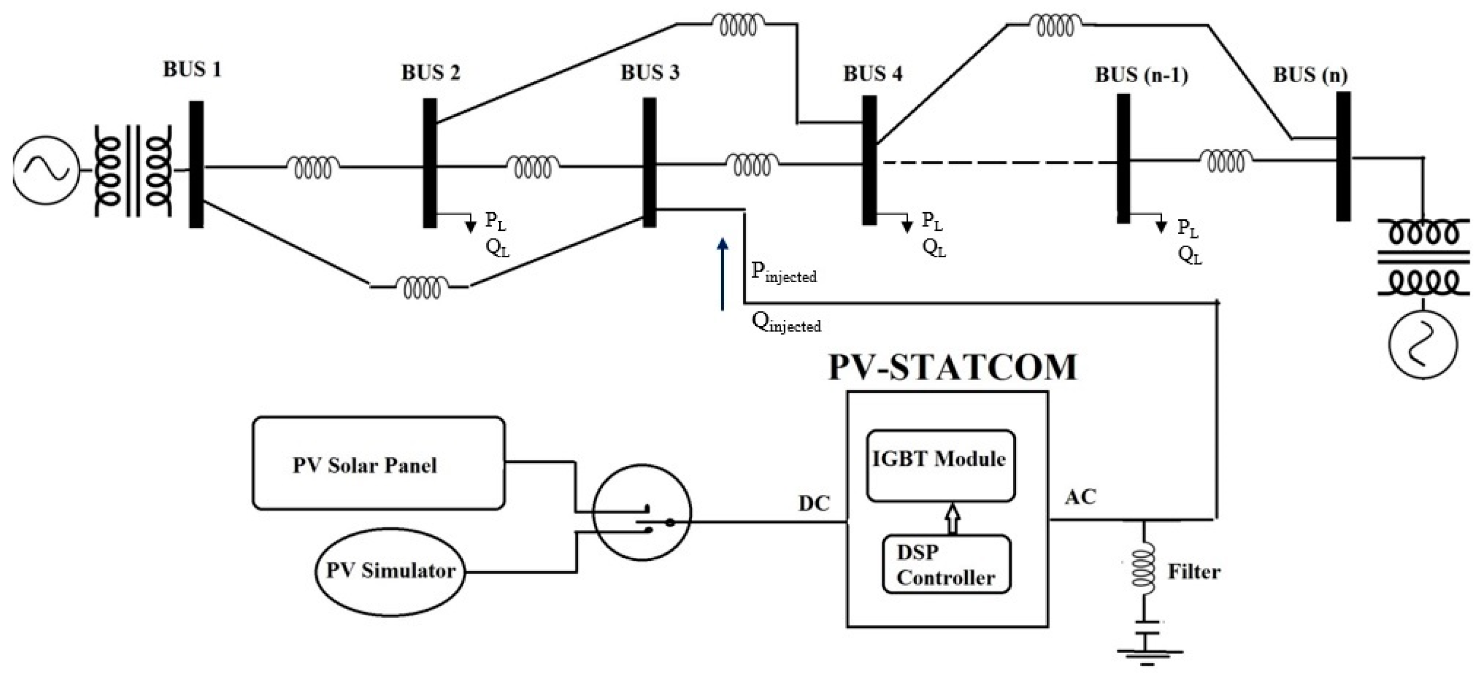
Another PV-STATCOM model was proposed in [9] as a voltage control with auxiliary damping control for increasing the transient stability and, consequently, the power transmission limit. The results demonstrated that a PV-STATCOM was not only applicable in distribution networks but that it can also substantially improve the stable transmission limits during both the day and night, even while generating tens of megawatts of real power [9]. The topology of a PV-STATCOM device connected to a transmission system is illustrated in Figure 1.
The benefits of active/reactive power compensation greatly depend on the placement and size of the added controllers. Although there are many different models proposed for new applications and constraints of PV-STATCOM, there are only a few published studies about the optimal placement and sizing of this device in a power system. In [10], an optimal distributed generation placement and sizing of a PV solar farm utilized as a STATCOM was proposed which concerned the necessity of fast reactive power compensation during voltage recovery processes under voltage sag or post-fault conditions. By adding weighted voltage support ability index analysis to the distributed generation planning constraints, the problem was solved to minimize the total annual cost.
In the present paper, a simple, novel method of optimal PV-STATCOM placement and sizing is proposed using empirical data. If solar irradiance data, solar power generation data and load data for all 8760 h of the year for a specific case study are available, then by modelling the active and reactive power of a PV-STATCOM in all time intervals, we can find the maximum portion of load that should be considered in the simulation. After that, we can find the candidate buses by calculating and sorting the power loss index, and finally, we can use an optimization technique to find the optimum PV-STATCOM size for those candidate buses.
The case study selected for this research is the power network of Northern Cyprus, which has quite high, almost uniform solar irradiation in all regions. In the Turkish Republic of Northern Cyprus (TRNC), the demand for electrical energy keeps increasing, and consequently, so does its price. However, the quality and price of electrical energy should be maintained at an optimum level. Unfortunately, electrical energy authorities in the TRNC have not set rules or regulations for reactive power compensation, and as a result, voltage drop, harmonics, overvoltage, noises and unnecessary reactive power on lines often occur. In fact, these cause a lack of quality electricity [11].
In this study, a multi-objective function is considered to minimize total power loss, voltage deviation and cost; the results of the optimal placement and sizing of one PV-STACOM using three different optimization techniques are also presented and compared.
The results show that installing one PV-STATCOM in a system can produce a greater reduction in power loss and voltage deviation than installing only one solar farm or only one STATCOM. In this study, the installation costs of a PV solar farm and a PV-STATCOM are also approximated, according to their size. Since PV-STACOM can both generate active power and improve the system power quality, its annual profit is much higher than a PV solar farm.
2. Objective Function
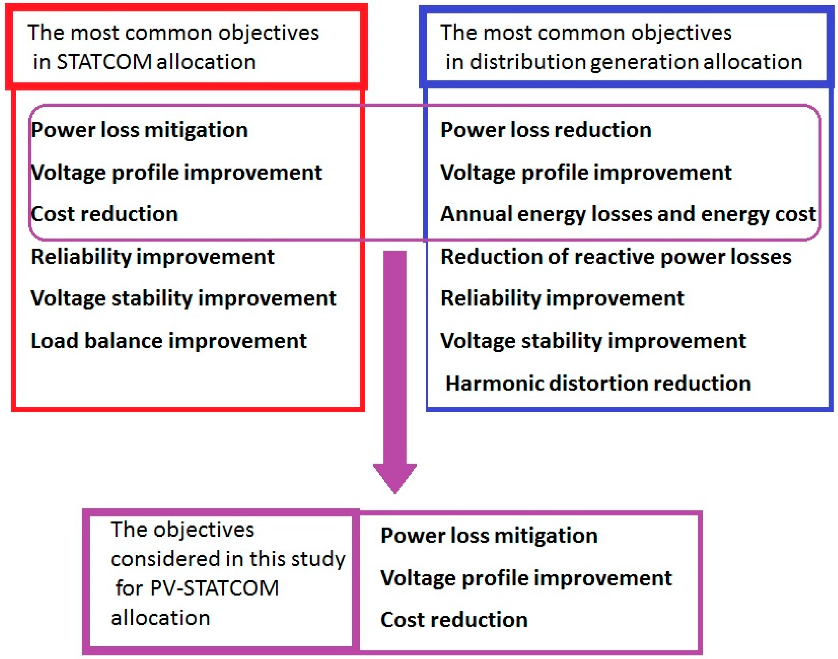
In the literature, there are too many publications in the field of optimal allocation of STATCOM in the power systems with different objective functions [12,13]. Moreover, in the examination of solutions for the problem of distributed generation placement and sizing, various objective functions have been presented in numerous publications [14]. The most common objectives which have been considered for two problems of optimal distributed generation allocation and optimal STATCOM placement are presented in Figure 2. Among these objectives, active power loss mitigation, voltage improvement and cost reduction are considered in this study for optimal PV-STATCOM placement and sizing. The objectives which are related to system dynamic support can be evaluated in the future works.
A multi-objective function is considered in searching for an optimal solution which minimizes power loss, voltage deviation and cost, described as follows.
2.1. Active Power Loss
In a power system, the total power loss is given by [12,15], as follows:
where b is the number of lines, and Rl and Il are the resistance and the current, respectively, through line l. Vi and θi are, respectively, the voltage magnitude and angle at bus i, and Yij and ϕij, respectively, are the magnitude and angle of the line admittance.
2.2. Voltage Deviation
The index of improvement of the voltage of a power system is defined as the deviation from the amplitude of the unit voltage on a bus. Thus, for a given system, the index of improvement of the voltage is given by [15]:
where n is the number of buses, ViN is the nominal voltage at bus i and Vi is the actual voltage at bus i. The nominal voltage is considered as 1 p.u in this study.
2.3. Investment Cost
A PV-STATCOM is an expensive device, and therefore, the investment cost for installing such controllers must be considered to justify the economic viability of the devices. In order to evaluate the profitability of PV-STATCOM owners a cost function should be taken into account. To calculate the cost of a PV-STATCOM, the following equation can be defined:
where Eloss is the total energy loss. Ke is average price of the unsold energy. Ka and Kb are yearly depreciation of installation and the maintenance costs of PV-STATCOM, respectively. Bj is defined as a binary variable and is equal to 1 if a PV-STATCOM is present at bus j and to 0 if no PV-STATCOM is present. SPV-STATCOM is the size of PV-STATCOM.
2.4. Operational Constraints
For optimal placement and sizing of PV-STATCOM, the following constraints are considered [12].
2.4.1. Power Flow Balance Equations
The power balance with respect to a bus can be formulated as:
where PGi and QGi, respectively, are the generated real and reactive powers, and PLi and QLi, respectively, are the load real and reactive powers at bus i. The conductance G’ik and the susceptance B’ik represent the real and imaginary components of element Y’ij in the bus admittance matrix.
2.4.2. Size Limit
The apparent power of a PV-STATCOM as an active/reactive power compensator must not exceed its limiting value:
2.4.3. Bus Voltage Limits
Bus voltages must be maintained within the limits of their nominal value given by:
In practice, the difference can reach 10% of the value of the voltage [12].
2.5. Fitness Function
An overall fitness function, in which each objective function is normalized with respect to the base system without a PV-STATCOM, is considered. This fitness function is given by:
subject to:
where Ploss, Lv and CostPV-STATCOM are the total active power loss, voltage deviation index and total cost, respectively. ω1, ω2 and ω3 are the coefficients of the corresponding objective functions, is the total active power loss in the network of the base case before installing PV-STATCOM, is the total voltage deviation of the base case and CostMax is the maximum allowed cost.
Considering Equation (3), the cost function consists of two terms. In the first term, the total energy loss is the product of total power loss and 8760 h of a year. In the other words, in the cost function, Eloss is directly proportional to Ploss which has been already considered as the first objective function component of Equation (8). In addition, the second term of cost function in Equation (3), only varies by the change in size of PV-STATCOM. It means due to consideration of power loss in the fitness function of Equation (8), to avoid redundancy, for the case that we are installing only one PV-STATCOM on the system and the size of that single additional device is determinative, rather than considering the cost of PV-STATCOM, it is reasonable to consider its size. In this way, all objectives will be taken to account by a small modification in the fitness function. Hence, in this study, the third objective function component of Equation (8), has been defined to have the minimum possible PV-STATCOM sizes regarding the control of a PV-STATCOM instead of considering the total PV-STATCOM cost. Since, in this study, only one PV-STATCOM has been considered, it is reasonable that:
where SPV-STATCOM is the PV-STATCOM size in MVA, and Smax is the maximum possible PV-STATCOM size, defined as its maximum apparent power.
According to the importance of any objective function component, the coefficients of ω1, ω2 and ω3 are different. In this study, due to importance of power loss reduction and voltage improvement, we consider that ω1 = 40%, ω2 = 40% and ω3 = 20%.
3. Power Loss Index
The power loss in transmission lines between buses i and j can be given by the following equation:
where Ploss and Qloss, respectively, are the active and reactive power losses. Rij and Xij, respectively, are the resistance and reactance of the line connected to the buses i and j, Pj and Qj are the real and reactive powers of the load at bus j, and Vj is the voltage magnitude at bus j [16].
Since we only consider real power loss minimization in the objective function, we can define the power loss index as follows [17].
For the case :
The power loss index is used to specify which buses are candidates to be a critical bus in the system in order to select locations at which to install a PV-STATCOM. The buses with higher power loss index values are critical buses; therefore, these will be suitable locations at which to install a PV-STACOM.
4. Adaptive Particle Swarm Optimization (APSO)
Particle swarm optimization (PSO) is a metaheuristic optimization technique based on populations inspired by bird flocking and fish schooling [15]. Initially, PSO was used to solve continuous nonlinear optimization problems, but it has now been extended to solutions of constrained nonlinear optimization problems with both discrete and continuous variables [18,19]. The basic idea behind the PSO algorithm is that a population called a swarm is generated randomly. The swarm is made up of individuals called particles, where each particle in the swarm represents a potential solution to the problem under consideration. Each particle moves through a dimensional search space at a random velocity. A particle updates its velocity and position according to the following equations:
where w is the inertia weight, c1 and c2 are acceleration constants, r1 and r2 are two random numbers in the range of [0,1], pbestik is the best position ever visited by a particle i at the kth iteration and gbestik is the global best position in the entire swarm.
The implementation of the PSO algorithm can be described by the following steps [18]:
- Step 1: Randomly initialize a swarm of particles in a D-dimensional search space.
- Step 2: Evaluate the fitness of the entire swarm.
- Step 3: Record the best position of each particle, pbest, and the global best position, gbest.
- Step 4: Update the velocity vector and position vector of each particle.
- Step 5: Repeat steps 2–4 until a stopping criterion is satisfied.
A global search can be facilitated by a large inertia weight, while a local search can be facilitated by a small inertia weight. In an adaptive version of PSO, the inertia weight can be updated dynamically by increasing the number of iterations [20]:
where Wmax and Wmin, respectively, are the upper and lower bounds of the inertia weight. This modification can increase the speed of convergence in conventional PSO.
5. Proposed Method for Optimal PV-STATCOM Placement in a Power Network
A PV-STATCOM is a device added to a power network which can inject active power in the daytime period and inject reactive power during the night. Since the apparent power of this device is constant, there is always a specific mathematical relationship between the amounts of active and reactive power injected into the system. The active power depends on the power generated by the solar power system, and the reactive power can be computed as:
where S is the PV-STATCOM apparent MVA power, P is the active power in MW produced by PV, and Q is the reactive power of the controller in MVar.
In Figure 3 and Figure 4, two samples of active/reactive power injected by a PV-STATCOM are presented for 24-h periods of different days. Figure 3 shows solar power production through a summer day, where active power of up to 800 kW can be generated. Figure 4 shows solar power production through a winter day, where active power of up to 520 kW can be generated, while the solar generation curve has fluctuations. For both figures, the reactive power graphs have been drawn.
Apart from the shape of the solar power production graphs, there are two points, indicated by stars, at which the amounts of the active and reactive powers are equal, or Q = P. The times during which Q = P in a PV-STATCOM are a few hours before and a few hours after the maximum solar irradiance time.
In the problem of the optimal placement and sizing of a PV-STATCOM, the capacity of the PV-STACOM is defined as its apparent power, but we do not know the amount of apparent power to calculate Q in each step; thus, we use the Q = P points, above, to try to find the apparent power, as follows:
in which Q (PV-STATCOM) = P (PV-STATCOM).
S (PV-STATCOM) = P(PV-STATCOM) + j Q (PV-STATCOM),
At the Q = P points, the load is a portion of the maximum load. There is no need to consider the given peak load of the case study when doing the power flow calculation. The load ratio in Q = P points can be defined as:
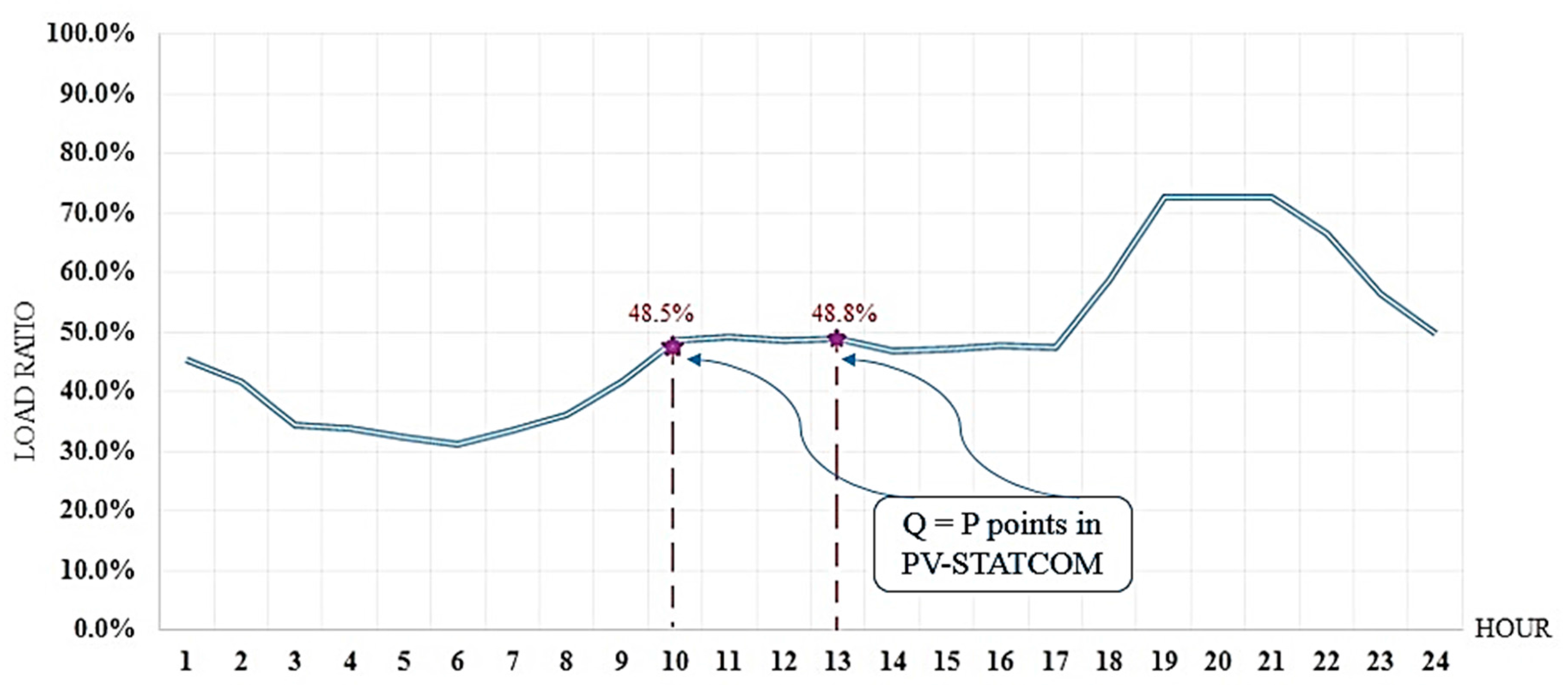
Figure 5 and Figure 6 are showing the graphs of load ratio in different time intervals for two different days which were already considered in Figure 3 and Figure 4, respectively. In Q = P points, the load ratio (LR) is obtained and shown. The highest LR on 22/08/2012 was 67.9% which happened on 4:00 p.m. and the maximum LR on 14/02/2012 was 48.8% that happened on 1:00 p.m. Annual peak load for the case study was considered as 313 MW using the load data.
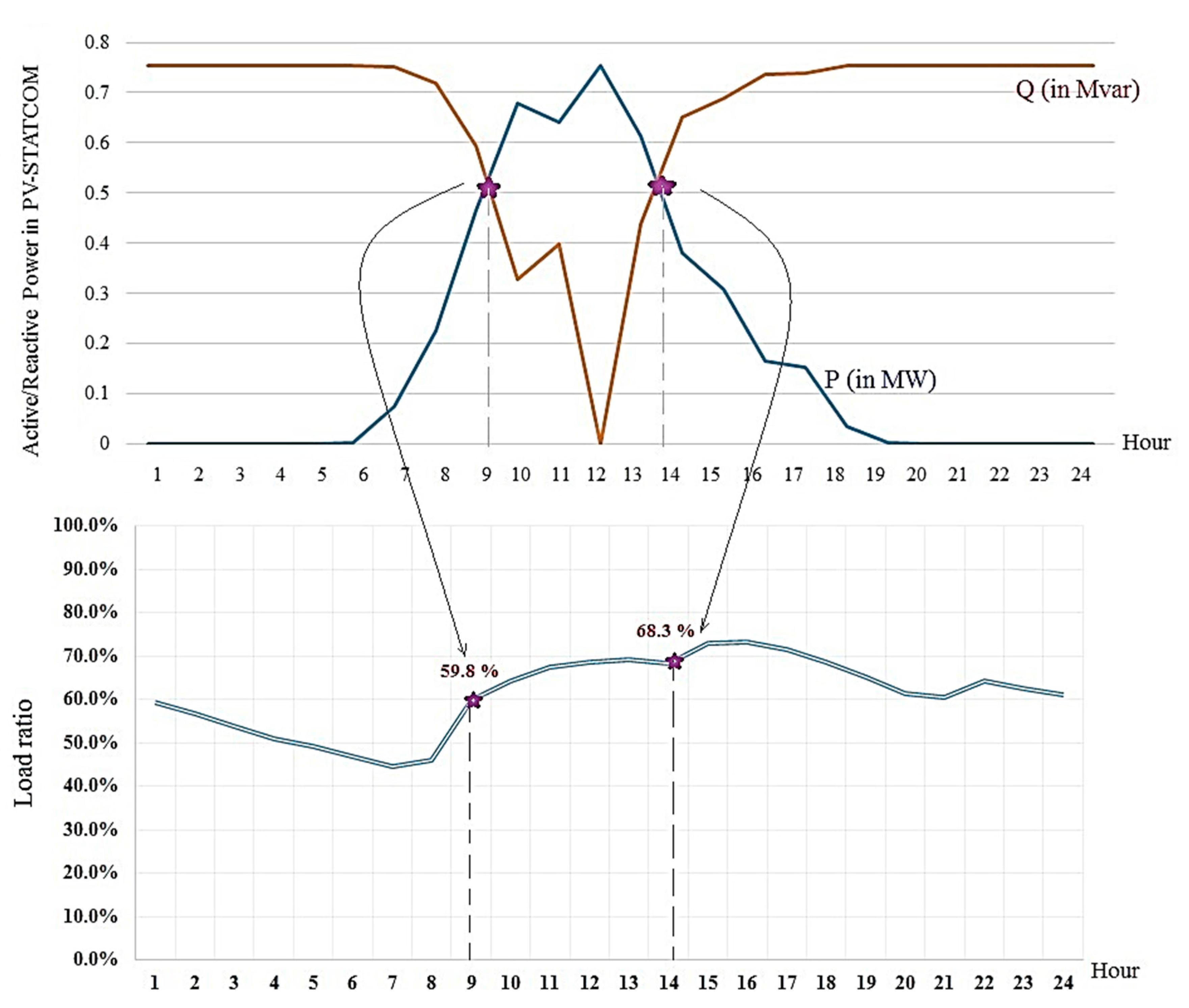
After finding all Q = P points for different days of the year and considering the load ratio in those points, the maximum LR value in Q = P points were obtained as 68.3% which was happened on 29 June 2012 at 2:00 p.m. as shown in Figure 7. The given peak load in the case study should be reduced by this LRmax.
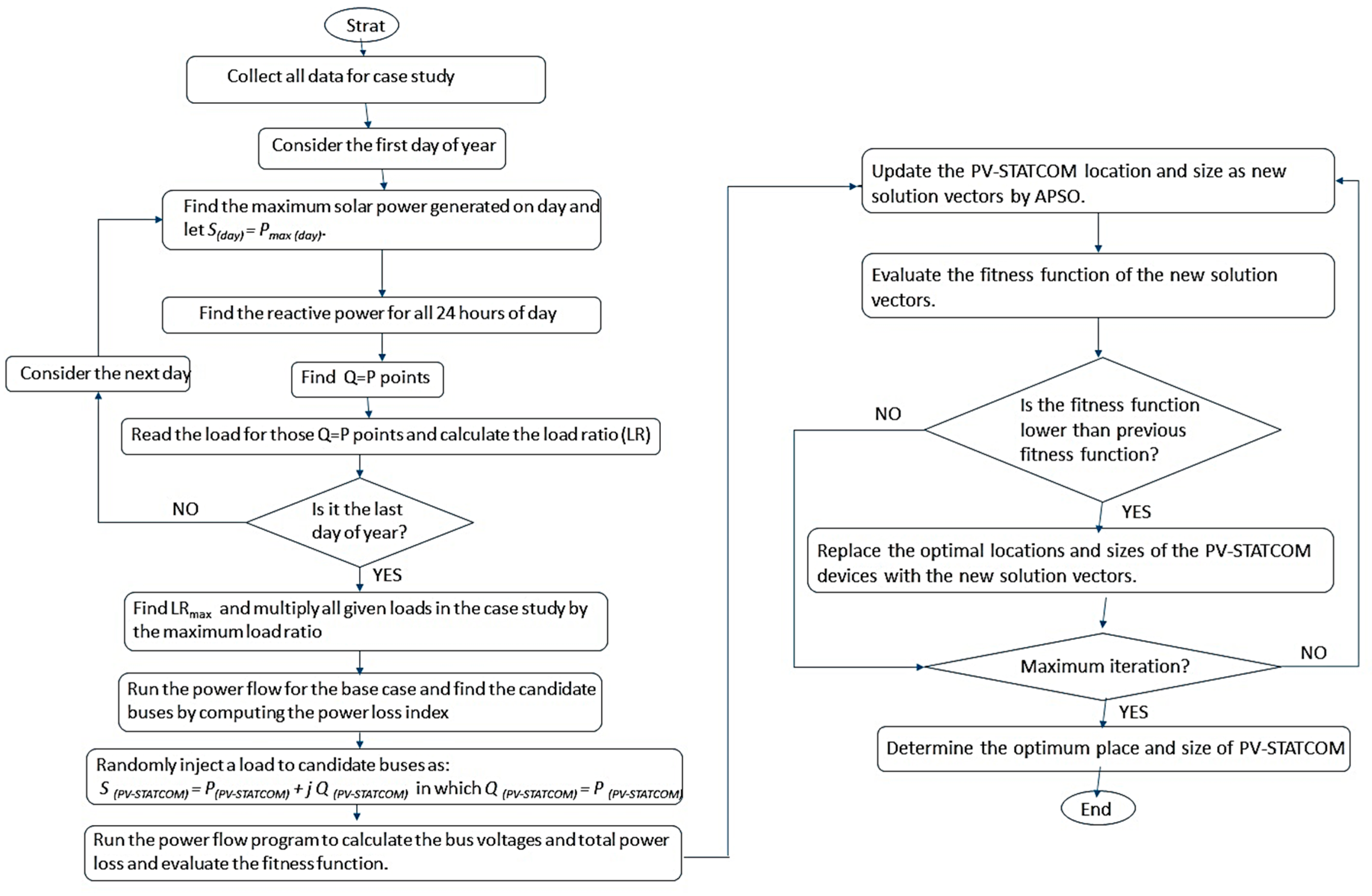
The proposed procedure for the optimal placement and sizing of a PV-STATCOM in a power network, when we have all data in terms of solar power production and load for 8760 h of a year for a specific case study, is as follows:
- (1)
- Collect all solar irradiance data, solar power generation data and load data for all 8760 h of a year for the case study.
- (2)
- Consider a day in the year, find the maximum solar power generated on that day (Pmax (day)) and suppose that the apparent power of that day is constant as S(day) = Pmax (day).
- (3)
- Find the reactive power for all 24 h of that day by
- (4)
- Find two time intervals of a 1-hour period in that day in which has the smallest value. Read the load for those time intervals and calculate the load ratio as
- (5)
- Repeat steps 2 to 4 for all days of a year and find the maximum LR value among all calculated LRs of different days of the year, as LRmax.
- (6)
- Multiply all given loads in the case study by the maximum load ratio of LRmax and run the power flow for the base case.
- (7)
- Find the candidate buses for installing a PV-STATCOM by computing the power loss index.
- (8)
- Randomly inject a load to candidate buses as:in which Q (PV-STATCOM) = P (PV-STATCOM).S (PV-STATCOM) = P(PV-STATCOM) + j Q (PV-STATCOM)
- (9)
- Run the power flow program to calculate the bus voltages and total power loss.
- (10)
- Evaluate the fitness function.
- (11)
- Update the PV-STATCOM location and size as new solution vectors through the optimization technique.
- (12)
- Evaluate the fitness function of the new solution vectors.
- (13)
- Check whether the PV-STATCOM set (i.e., the new solution vector) has a lower fitness function value than the previous solution vector. If yes, the optimal locations and sizes of the PV-STATCOM devices are replaced with the new solution vectors. Otherwise, go to step 11.
- (14)
- Determine the optimum PV-STATCOM placement and sizing which provides minimum power loss, voltage deviation and total cost.
Figure 8 describes the proposed procedure in terms of flowchart.
6. Case Study and Results
The case study in this paper is the electrical transmission network in Northern Cyprus, which has 23 substations as shown in Figure 9. The total power generated in the system is 345 MW. There are two types of transmission lines, depending on the voltage rate, the first being 132 kV and the second 66 kV.
The five most critical buses with high power loss index values are illustrated in Table 1. These buses are suitable for installing a PV-STATCOM. The problem of the optimal placement and sizing of PV-STATCOM devices will be solved to find the best size to be installed on a bus among these critical buses.
All solar irradiance data, solar power generation data and load data for all 8760 h of a year were available for this case study [22]. The maximum load ratio value among all calculated LRs of different days of the year in Q = P points were obtained, as LRmax = 0.683. This meant that the given peak load in the case study should be reduced by 68.3%. In the new load condition, we ran the power flow to obtain the results for the base case without any PV-STATCOM, and afterwards, we conducted the procedure proposed in the previous section in order to find the best location and size of PV-STATCOM at the candidate buses. The total power loss in the base case with the new load condition was obtained as 9.75 MW, and the voltage deviation was 0.249. The maximum apparent power of the PV-STATCOM was supposed to be 2 MVA. Using the base case values, the fitness function could be calculated in each iteration.
For a fair comparison of the results—since the concept of ‘particle and population’ in PSO is very similar to the term ‘scot bee and colony’ in bee colony optimization (BCO) [23] and also to the term ‘projectile and step leader’ used in the lightening search algorithm (LSA) [24], BCO and LSA were also selected for this study [25]. The optimal parameters of these three optimization techniques are shown in Table 2.
The results for the optimal placement and sizing of one PV-STACOM device, using the three different optimization techniques, were obtained and are presented in Table 3. The optimum locations and sizes of PV-STATCOM devices, obtained by these different methods, differ from each other. The size of PV-STATCOM in terms of apparent power is calculated by
where PPV-STATCOM and QPV-STATCOM are the optimum values of active and reactive power obtained by optimization techniques and they are both equal to each other.
Among these three optimization techniques, the results of APSO in terms of power loss reduction, voltage improvement and fitness function value were better. The size for PV-STATOM obtained by PSO was higher than the values obtained using the other objective function components. Even the computational time using APSO was smaller, which meant that the APSO algorithm produced better results in terms of accuracy and speed in optimal PV-STATCOM placement and sizing.
By considering different objective function coefficients in Equation (8), the proposed algorithm is implemented and the obtained results are presented in Table 4. According to the importance of any objective function component, the coefficients of ω1, ω2 and ω3 are different. We can see the lowest fitness function value is for the case that ω1 = 40%, ω2 = 40% and ω3 = 20%.
Then we considered and compared the results of three cases as follows:
- Case 1: Installing only one solar farm in the system, in which |S| = PPV and QSTATCOM = 0.
- Case 2: Installing only one STATCOM in the system, in which |S| = QSTATCOM and PPV = 0.
- Case 3: Installing PV-STATCOM in the system, in which
A comparison of the results for these three cases obtained by APSO is presented in Table 5. The results show that installing one PV-STATCOM at GIRNE II can reduce power loss and voltage deviation to a greater extent than the cases of installing only a solar farm or only a STATCOM.
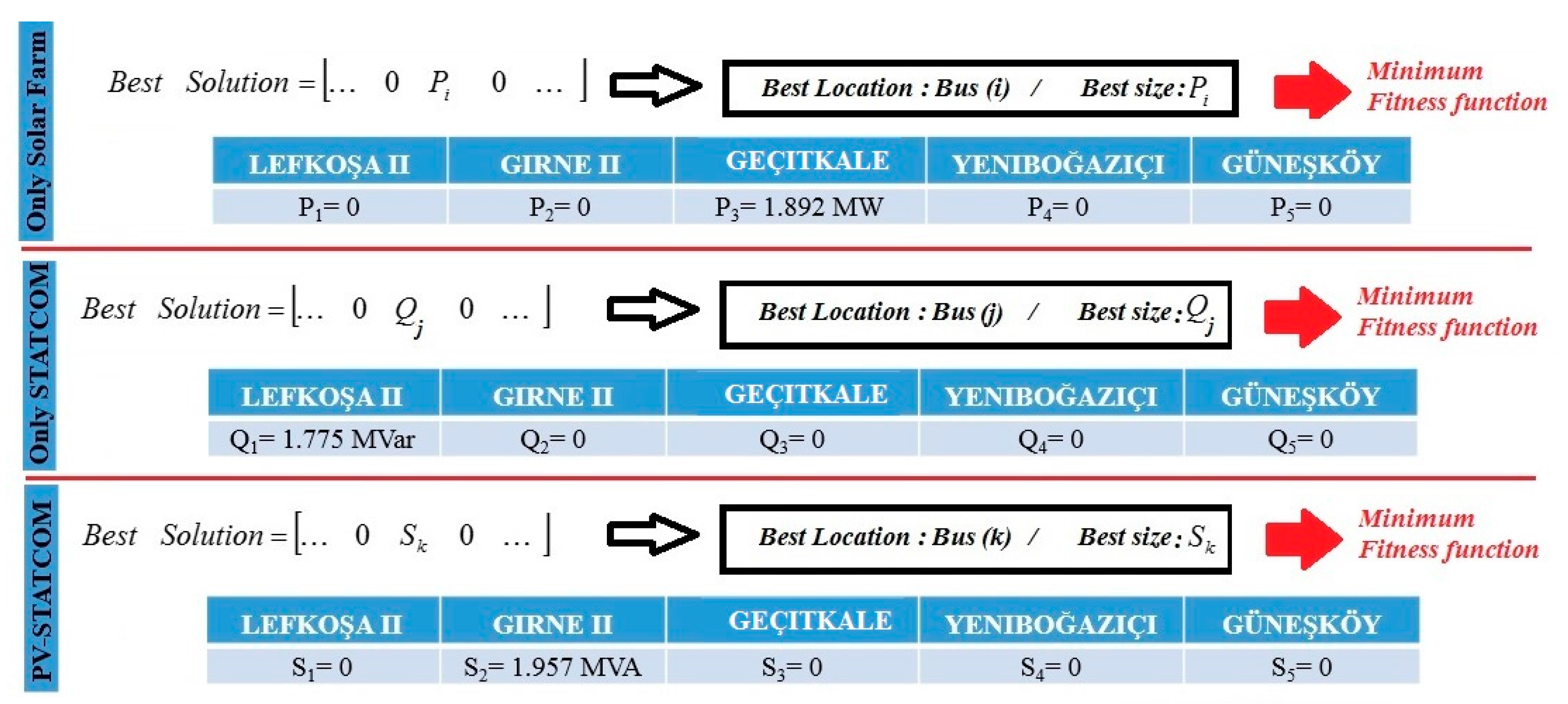
Since five busbars have been selected as the most critical buses with high power loss index, the best solution to be found by the proposed optimization algorithm is a (1 × 5) matrix where four arrays values are 0. A value of 0 in the matrix means that there is no need to install any additional device at that bus. Consider the best solutions shown in Figure 10 which are obtained for different cases. For any case, the best solution is a (1 × 5) matrix which has only one nonzero array. That array shows the best location and size of the additional devices.
The solutions indicate that the best solar farm, STATCOM and PV-STATCOM placement are at buses i, j, k, respectively. Moreover, the best solar farm, STATCOM and PV-STATCOM sizes are Pi, Qj and Sk, respectively. The optimal solution in all cases leads to maximum power loss reduction, minimum voltage deviation, considering the size of additional components.
In Table 6, the installation cost of each additional device according to its size is approximated for case 1 and case 3. The installation cost of one PV solar farm is considered as 1.2 USD/W while the installation costs of one PV-STATCOM have been approximated using Ref. [26]. From these installation costs, we can see that if the installed solar farm used as PV-STATCOM, the cost of installing a solar farm and after utilizing as PV-STATCOM would be around 100,000 USD. In comparison to the cost of installing a separate STATCOM in [23]; this is certainly more reasonable.
In addition, yearly depreciation of the installation and the maintenance costs, yearly profit by power loss reduction and yearly earning by sold energy for these two case are obtained as shown in Table 6. Consequently, the annual profits of using a single solar farm and a PV-STATCOM are presented and compared. Since PV-STACOM can both generate active power and improve the system power quality, its annual profit is much higher than using a single solar farm.
7. Conclusions
Recently, the concept of utilizing a PV solar farm inverter as a STATCOM during the night has been proposed. According to this concept, during the night, the entire inverter capacity would be utilized for a STATCOM, while during the day, the remaining inverter capacity would be utilized for a STATCOM. Increasing the utility of a PV solar farm, engaging in acceptable voltage regulation, improving the power factor and electrical system performance and providing additional revenue earnings for solar power system owners during both the day and night are only some of the objectives to be achieved by using PV-STATCOM in power systems. In this paper, a simple, novel method for optimal PV-STATCOM placement and sizing was proposed which used empirical data. The maximum load ratio needed was found from the solar irradiance and load data and was used instead of the peak load. The two sub-problems of placement and sizing were solved, respectively, by the power loss index and adaptive particle swarm optimization, considering the objectives of power loss and cost minimization as well as voltage improvement. The obtained results for the power network of Northern Cyprus, which has quite high and almost uniform solar irradiation in all regions, showed that installing one PV-STATCOM in the system can reduce power loss and voltage deviation to a greater extent than installing one solar farm alone or one STATCOM alone. The annual profit of installing PV-STATCOM is much higher than using solar farm. The problem of optimal PV-STATCOM placement and sizing in both transmission and distribution systems considering the effect of harmonics and the objectives which are related to system dynamic support can be evaluated in the future works.
Acknowledgments
The author would like to thank the electric company of Northern Cyprus (KIBTEK) for the information given.
Conflicts of Interest
The author declares no conflict of interest.
References
- Gayatri, M.T.L.; Alivelu, M.; Parimi, A.V.; Pavan, K. A review of reactive power compensation techniques in microgrids. Renew. Sustain. Energy Rev. 2018, 81, 1030–1036. [Google Scholar] [CrossRef]
- Kevin Schönleber, K.; Collados, C.; Teixeira Pinto, R.; Ratés-Palau, S.; Gomis-Bellmunt, O. Optimization-based reactive power control in HVDC-connected wind power plants. Renew. Energy 2017, 109, 500–509. [Google Scholar] [CrossRef]
- Jordehi, A.R. Optimal allocation of FACTS devices for static security enhancement in power systems via imperialistic competitive algorithm (ICA). Appl. Soft Comput. 2016, 48, 317–328. [Google Scholar] [CrossRef]
- Sirjani, R.; Mohamed, A.; Shareef, H. Comparative study of effectiveness of different var compensation devices in large-scale power networks. J. Cent. South Univ. 2013, 20, 715–723. [Google Scholar] [CrossRef]
- Varma, R.K.; Khadkikar, V.; Seethapathy, R. Nighttime application of PV solar farm as STATCOM to regulate grid voltage. IEEE Trans Energy Convers. 2009, 24, 983–985. [Google Scholar] [CrossRef]
- Varma, R.K.; Rangarajan, S.S.; Axente, I.; Sharma, V. Novel Application of a PV Solar Plant as STATCOM During Night and Day in a Distribution Utility Network. In Proceedings of the 2011 IEEE/PES Power Systems Conference and Exposition, Phoenix, AZ, USA, 20–23 March 2011; pp. 1–8. [Google Scholar] [CrossRef]
- Varma, R.K.; Das, B.; Axente, I.; Vanderheide, T. Optimal 24-hr Utilization of a PV Solar System as STATCOM (PV-STATCOM) in a Distribution Network. In Proceedings of the 2011 IEEE Power and Energy Society General Meeting, San Diego, CA, USA, 24–29 July 2011; pp. 1–8. [Google Scholar] [CrossRef]
- Varma, R.K.; Siavashi, E.M.; Das, B.; Sharma, V. Real-Time Digital Simulation of a PV solar system as STATCOM (PV-STATCOM) for voltage regulation and power factor correction. In Proceedings of the 2012 IEEE Electrical Power and Energy Conference, London, ON, Canada, 10–12 October 2012; pp. 157–163. [Google Scholar] [CrossRef]
- Varma, R.K.; Rahman, S.A.; Vanderheide, T. New control of PV solar farm as STATCOM (PV-STATCOM) for increasing grid power transmission limits during night and day. IEEE Trans Power Deliv. 2015, 30, 755–763. [Google Scholar] [CrossRef]
- Luo, L.; Gu, W.; Zhang, X.-P.; Cao, G.; Wang, W.; Zhu, G.; You, D.; Wu, Z. Optimal siting and sizing of distributed generation in distribution systems with PV solar farm utilized as STATCOM (PV-STATCOM). Appl. Energy 2018, 210, 1092–1100. [Google Scholar] [CrossRef]
- Özerdem, Ö.C.; Biricik, S.A. Research and Solution Proposal for Reactive Power Problems in North Cyprus Industries. In Proceedings of the 2009 International Conference on Electrical and Electronics Engineering—ELECO 2009, Bursa, Turkey, 5–8 November 2009. [Google Scholar] [CrossRef]
- Sirjani, R. Optimal placement and sizing of statcom in power systems using heuristic optimization techniques. In Static Compensators (STATCOMs) in Power Systems; Power Systems Series; Shahnia, F., Rajakaruna, S., Ghosh, A., Eds.; Springer: Singapore, 2015; pp. 437–476. [Google Scholar]
- Sirjani, R.; Jordehi, A.R. Optimal placement and sizing of distribution static compensator (D-STATCOM) in electric distribution networks: A review. Renew. Sustain. Energy Rev. 2017, 77, 688–694. [Google Scholar] [CrossRef]
- Jordehi, A.R. Allocation of distributed generation units in electric power systems: A review. Renew. Sustain. Energy Rev. 2016, 56, 893–905. [Google Scholar] [CrossRef]
- Sirjani, R.; Mohamed, A.; Shareef, H. Optimal allocation of shunt Var compensators in power systems using a novel global harmony search algorithm. Int. J. Electr. Power 2012, 43, 562–572. [Google Scholar] [CrossRef]
- Ali, E.S.; Abd Elazim, S.M.; Abdelaziz, A.Y. Improved harmony algorithm and power loss index for optimal locations and sizing of capacitors in radial distribution systems. Int. J. Electr. Power 2016, 80, 252–263. [Google Scholar] [CrossRef]
- Samimi, A.; Golkar, M.A. A novel method for optimal placement of FACTS based on sensitivity analysis for enhancing power system static security. Asian J. Appl. Sci. 2012, 5, 1–19. [Google Scholar] [CrossRef]
- Eajal, A.A.; El-Hawary, M.E. Optimal capacitor placement and sizing in unbalanced distribution systems with harmonics consideration using particle swarm optimization. IEEE Trans Power Deliv. 2010, 25, 1734–1741. [Google Scholar] [CrossRef]
- Liang, X.; Li, W.; Zhang, Y.; Zhong, Y.; Zhou, M. Recent Advances in Particle Swarm Optimization via Population Structuring and Individual Behavior Control. In Proceedings of the 2013 10th IEEE International Conference on Networking, Sensing and Control (ICNSC), Evry, France, 10–12 April 2013; pp. 503–508. [Google Scholar] [CrossRef]
- Zhan, Z.H.; Zhang, J.; Li, Y.; Chung, H.S.H. Adaptive particle swarm optimization. IEEE Trans Syst. Man Cybern B 2009, 39, 1362–1381. [Google Scholar] [CrossRef] [PubMed]
- KIB-TEK Transmission Development Plan. 2017. Available online: http://shewkee.com/kib-tek-iletim-sebekesi-planlanan-yatirimlar/ (accessed on 1 January 2018).
- The Electric Company of Northern Cyprus (KIBRIS TÜRK ELEKTRİK KURUMU). Available online: https://www.kibtek.com/ (accessed on 1 January 2018).
- Teodorović, D. Bee colony optimization (BCO). In Innovations in Swarm Intelligence. Studies in Computational Intelligence; Lim, C.P., Jain, L.C., Dehuri, S., Eds.; Springer: Berlin/Heidelberg, Germany, 2009; Volume 248. [Google Scholar]
- Shareef, H.; Ibrahim, A.A.; Mutlag, A.H. Lightning search algorithm. Appl. Soft Comput. 2015, 36, 315–333. [Google Scholar] [CrossRef]
- Sirjani, R.; Shareef, H. Parameter extraction of solar cell models using the lightning search algorithm in different weather conditions. J. Sol. Energy Eng. 2016, 138, 041007. [Google Scholar] [CrossRef]
- Varma, R.K.; Siavashi, E. Lab Validation of PV Solar Inverter Control as STATCOM (PV-STATCOM), IEEE-PES Presentation 2014. pp. 1–31. Available online: https://www.ieee-pes.org/presentations/td2014/td2014p-000714.pdf (accessed on 1 January 2018).
Figure 1.
Topology of a photovoltaic solar farm inverter as a static synchronous compensator (PV-STATCOM) device connected to a transmission system.
Figure 1.
Topology of a photovoltaic solar farm inverter as a static synchronous compensator (PV-STATCOM) device connected to a transmission system.


Figure 3.
Active/Reactive power of PV-STATCOM on 22 August 2012.
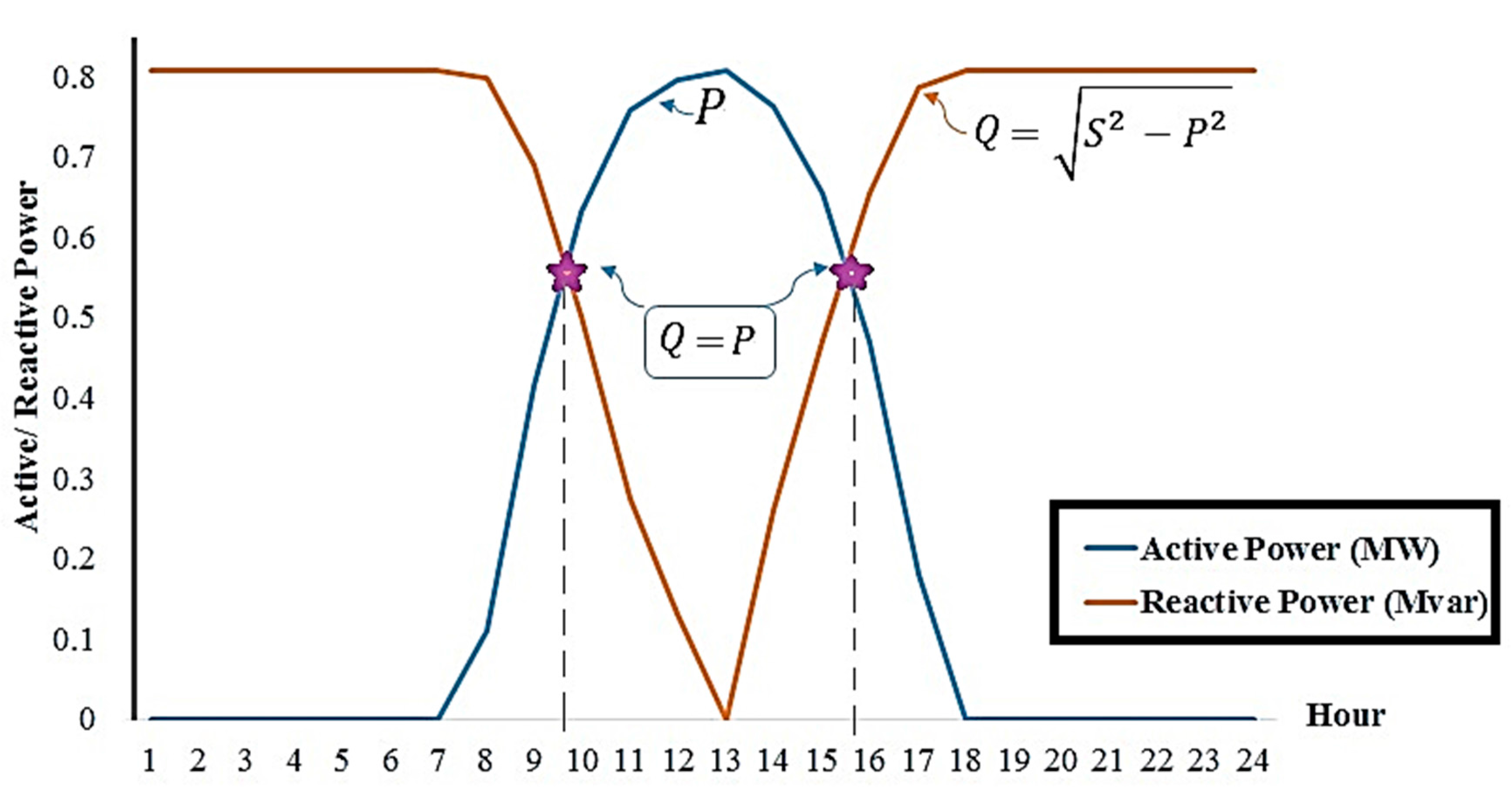
Figure 4.
Active/reactive power of PV-STATCOM on 14 February 2012.
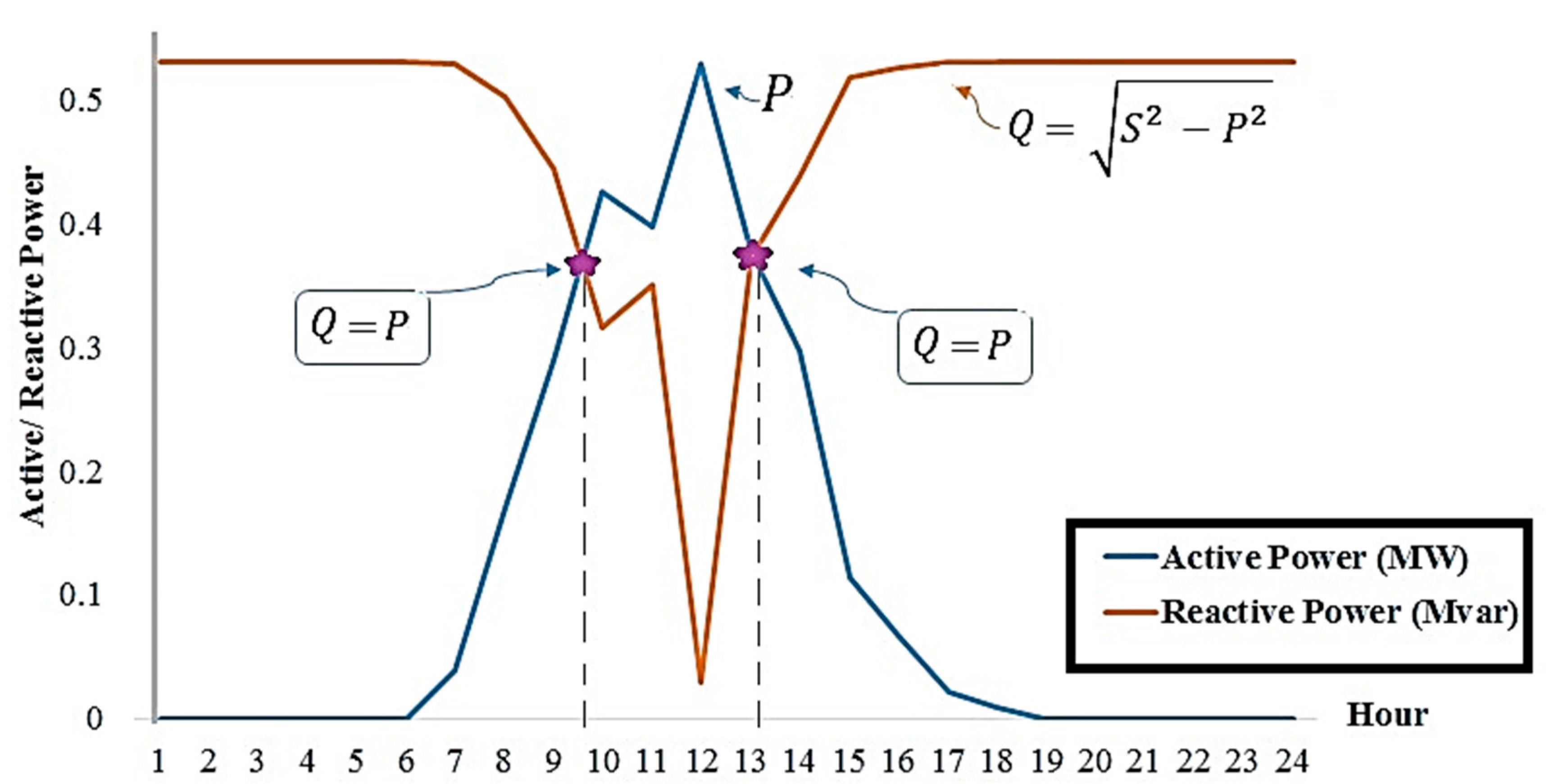
Figure 5.
Load ratio in different time intervals on 22 August 2012.
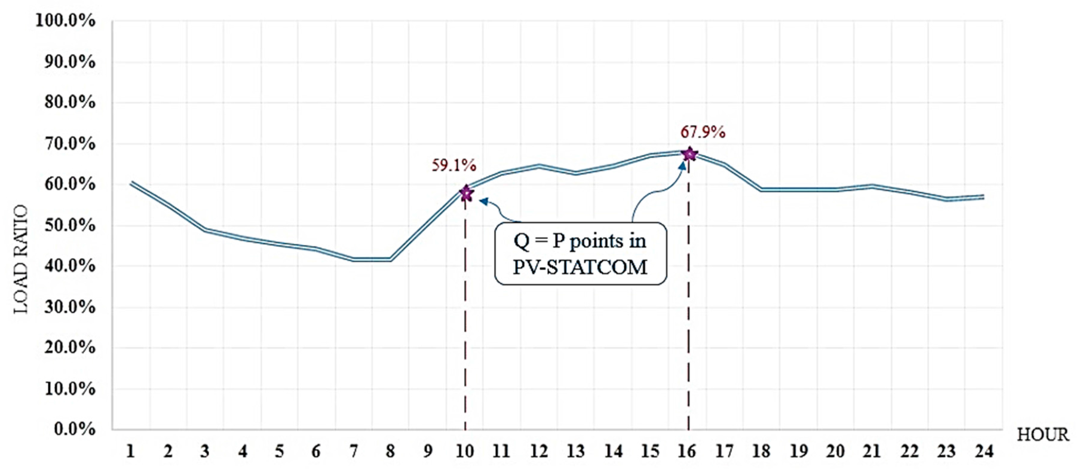
Figure 6.
Load ratio in different time intervals on 14 February 2012.

Figure 7.
The maximum load ratio in Q = P points among all days of year (on 29 June 2012).

Figure 8.
Flowchart of the proposed procedure.

Figure 9.
Northern Cyprus power network [21].
Figure 9.
Northern Cyprus power network [21].
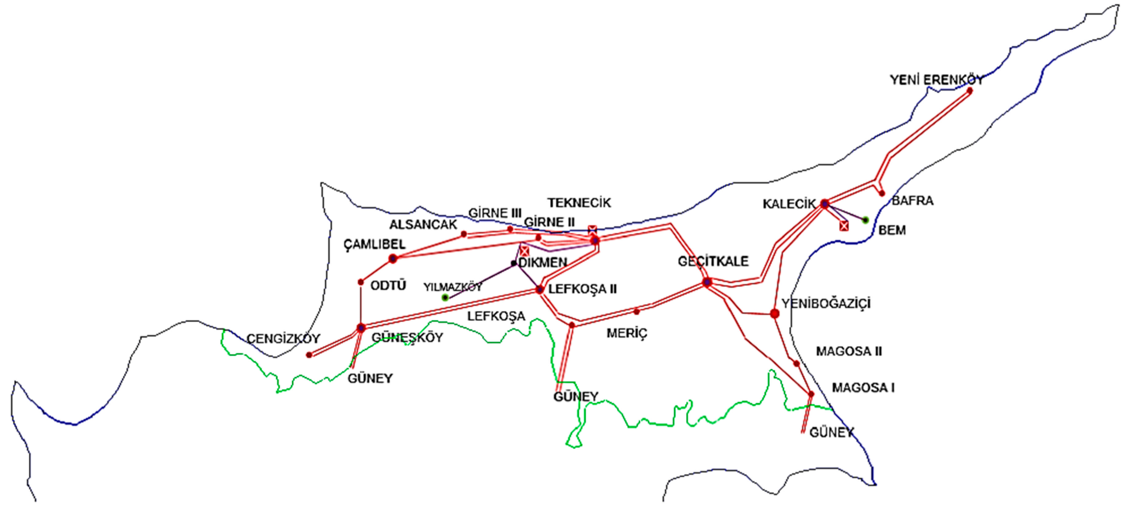
Figure 10.
Investigating the optimal solution for different cases.


Table 1.
The most critical buses with high power loss index.
| Substation Name | LEFKOŞA II | GIRNE II | GEÇITKALE | YENIBOĞAZIÇI | GÜNEŞKÖY |
|---|---|---|---|---|---|
| Power Loss Index | 0.8911 | 0.8518 | 0.7092 | 0.6787 | 0.6104 |
Table 2.
Optimal parameters of different optimization techniques.
| BCO | LSA | APSO | |||
|---|---|---|---|---|---|
| Run time | 5 | Maximum channel | 5 | Acceleration constants | 1.2 |
| Colony size | 25 | Step leader size | 25 | Population size | 25 |
| Number of iterations | 300 | Number of iterations | 300 | Number of iterations | 300 |
Table 3.
Comparison of the results of different techniques.
| Objective Function Components | Base Case | LSA | BCO | APSO |
|---|---|---|---|---|
| Location and Size | - | 1.872 MVA (at GÜNEŞKÖY) | 1.843 MVA (at LEFKOŞA II) | 1.957 MVA (at GIRNE II) |
| Total Power Loss (MW) | 9.75 | 9.39 | 9.57 | 9.31 |
| Voltage Deviation | 0.249 | 0.1898 | 0.2071 | 0.1641 |
| Fitness Function Value | 1 | 0.8773 | 0.9096 | 0.8412 |
| Computational Time (s) | - | 8.62 | 12.11 | 7.48 |
Table 4.
Comparison of the results the proposed algorithm using different objective function coefficients.
Table 4.
Comparison of the results the proposed algorithm using different objective function coefficients.
| ω1 | ω2 | ω3 | Best Size (MVA) | Best Location | Power Loss (MW) | Voltage Deviation | Fitness Function Value |
|---|---|---|---|---|---|---|---|
| 40% | 40% | 20% | 1.957 | GIRNE II | 9.31 | 0.1641 | 0.8412 |
| 35% | 35% | 30% | 1.812 | GIRNE II | 9.47 | 0.1732 | 0.8552 |
| 50% | 40% | 10% | 1.976 | LEFKOŞA II | 9.29 | 0.1673 | 0.8439 |
| 50% | 25% | 25% | 1.894 | GIRNE II | 9.33 | 0.2001 | 0.9161 |
| 25% | 25% | 50% | 1.643 | LEFKOŞA II | 9.56 | 0.2119 | 0.8686 |
Table 5.
Comparison of the results of three cases obtained by adaptive particle swarm optimization (APSO).
Table 5.
Comparison of the results of three cases obtained by adaptive particle swarm optimization (APSO).
| Items | Only Solar Farm | Only STATCOM | PV-STATCOM |
|---|---|---|---|
| Location and Size | 1.892 MW | 1.775 MVar | 1.957 MVA |
| (at GEÇITKALE) | (at LEFKOŞA II) | (at GIRNE II) | |
| Power Loss Reduction | 1.32% | 2.87% | 4.51% |
| Voltage Improvement | 8.53% | 22.45% | 34.01% |
Table 6.
Comparison of the costs of Case 1 and Case 3.
| Costs | Only Solar Farm | PV-STATCOM |
|---|---|---|
| Approximate Installation Cost | $2.3 Million | $2.4 Million |
| Yearly depreciation of the installation and the maintenance costs | $0.56 Million | $0.7 Million |
| Yearly profit by power loss reduction | $0.11 Million | $0.39 Million |
| Yearly earning by sold energy | $0.83 Million | $0.86 Million |
| Annual profit | $0.37 Million | $0.54 Million |
© 2018 by the author. Licensee MDPI, Basel, Switzerland. This article is an open access article distributed under the terms and conditions of the Creative Commons Attribution (CC BY) license (http://creativecommons.org/licenses/by/4.0/).
Share and Cite
MDPI and ACS Style
Sirjani, R. Optimal Placement and Sizing of PV-STATCOM in Power Systems Using Empirical Data and Adaptive Particle Swarm Optimization. Sustainability 2018, 10, 727. https://doi.org/10.3390/su10030727
AMA Style
Sirjani R. Optimal Placement and Sizing of PV-STATCOM in Power Systems Using Empirical Data and Adaptive Particle Swarm Optimization. Sustainability. 2018; 10(3):727. https://doi.org/10.3390/su10030727
Chicago/Turabian StyleSirjani, Reza. 2018. "Optimal Placement and Sizing of PV-STATCOM in Power Systems Using Empirical Data and Adaptive Particle Swarm Optimization" Sustainability 10, no. 3: 727. https://doi.org/10.3390/su10030727
Note that from the first issue of 2016, this journal uses article numbers instead of page numbers. See further details here.