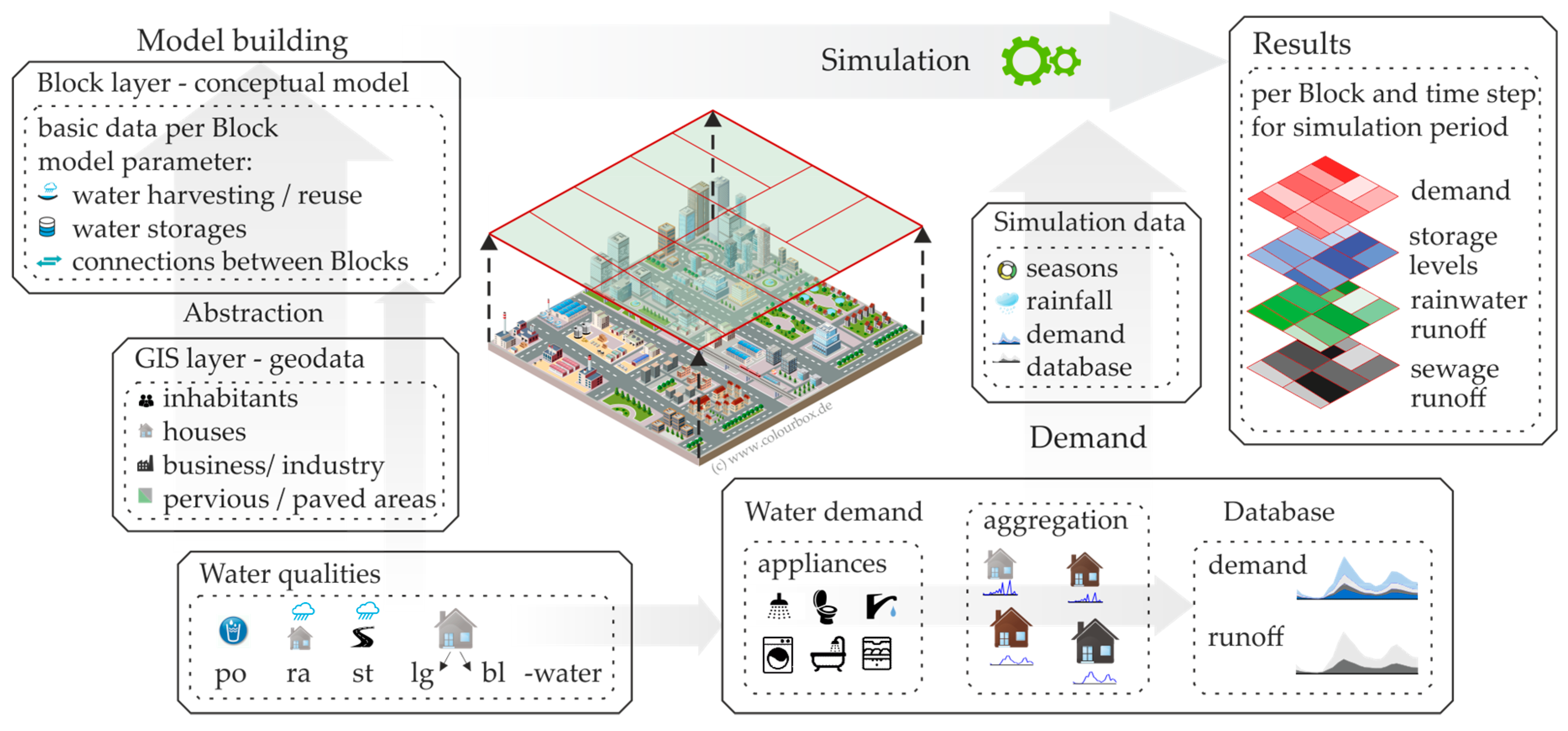
Figure 1.
Scheme of the model development: abstraction of detailed data to a conceptual model (assignment of water qualities—potable (po), rain (ra), storm (st), light grey (lg), and black (bl)—water—end-user water demand to Block demand curves, areal data to Block parameters and implementation of decentralised measures), simulation (with statistical data) and spatially presentation of the results.
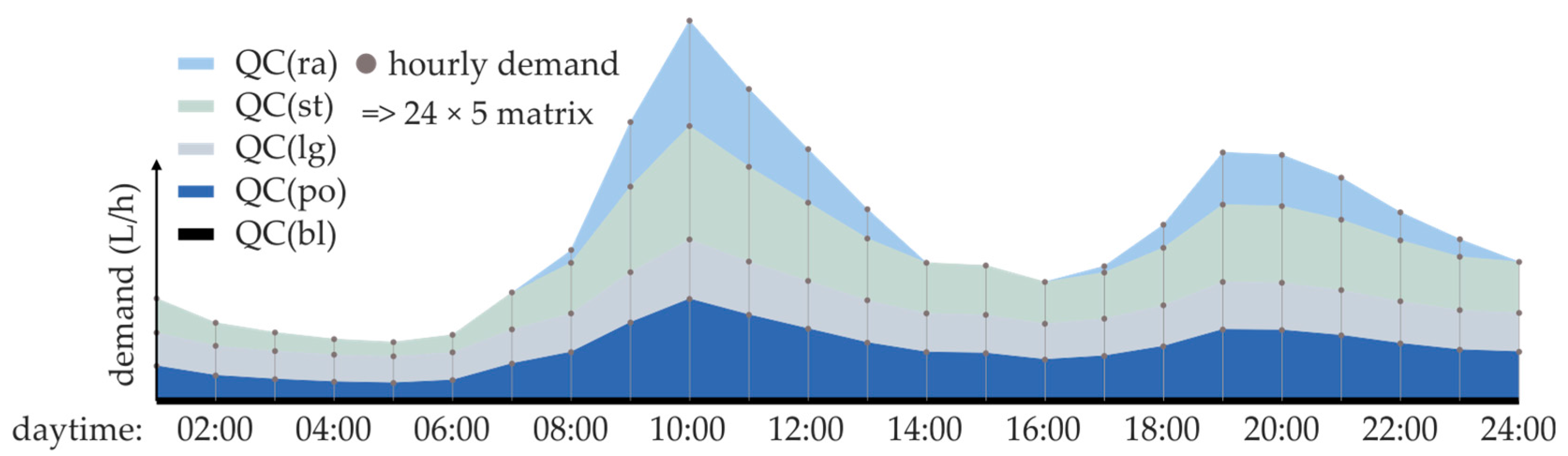
Figure 2.
Schematic example for a quality-based daily demand curve (DC) containing five Quality Classes (QC; QC(bl) = 0) over 24 h.
Figure 2.
Schematic example for a quality-based daily demand curve (DC) containing five Quality Classes (QC; QC(bl) = 0) over 24 h.
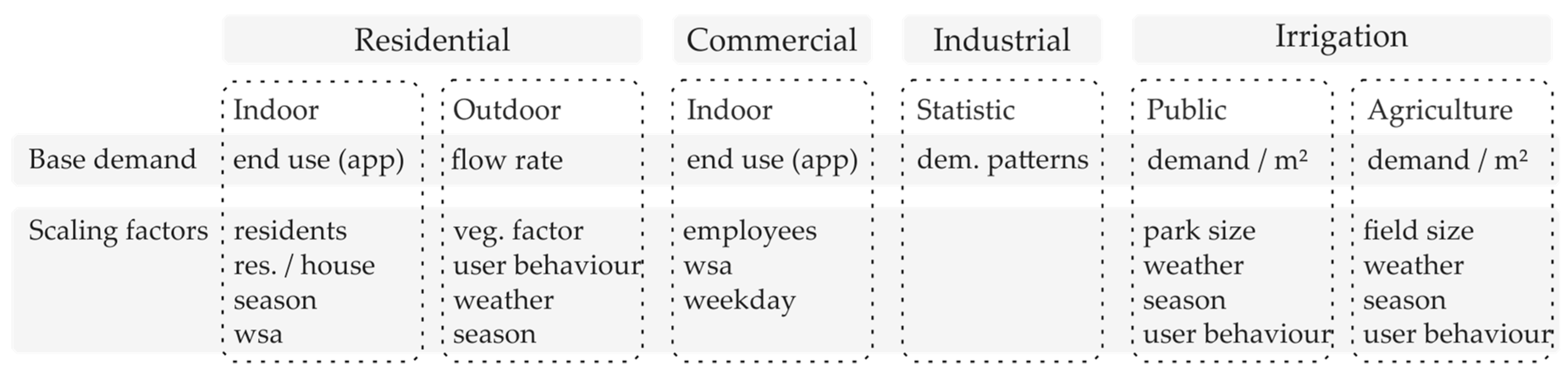
Figure 3.
Demand types (residential, commercial, industrial, and irrigation). The base demand originates from statistical data; scaling factors are Block-dependent parameters to assemble the individual Block demand.
Figure 3.
Demand types (residential, commercial, industrial, and irrigation). The base demand originates from statistical data; scaling factors are Block-dependent parameters to assemble the individual Block demand.
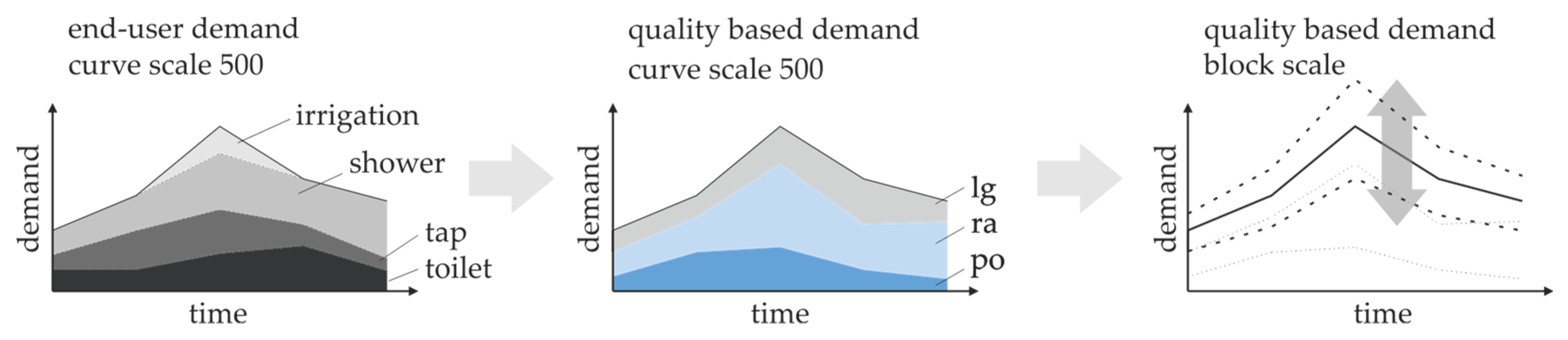
Figure 4.
From end-use demand to standard DC (curve scale of 500 people, schematic diagram) and scaled Block demand.
Figure 4.
From end-use demand to standard DC (curve scale of 500 people, schematic diagram) and scaled Block demand.
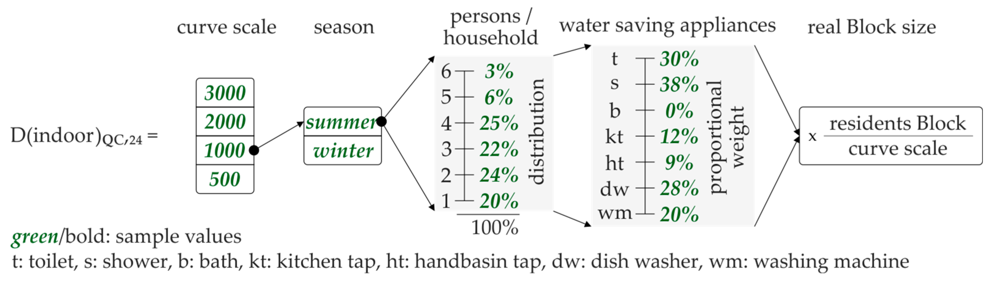
Figure 5.
Example for DC sampling (Curve scale: 1000 residents, summer, distribution of household size and water saving appliances).
Figure 5.
Example for DC sampling (Curve scale: 1000 residents, summer, distribution of household size and water saving appliances).
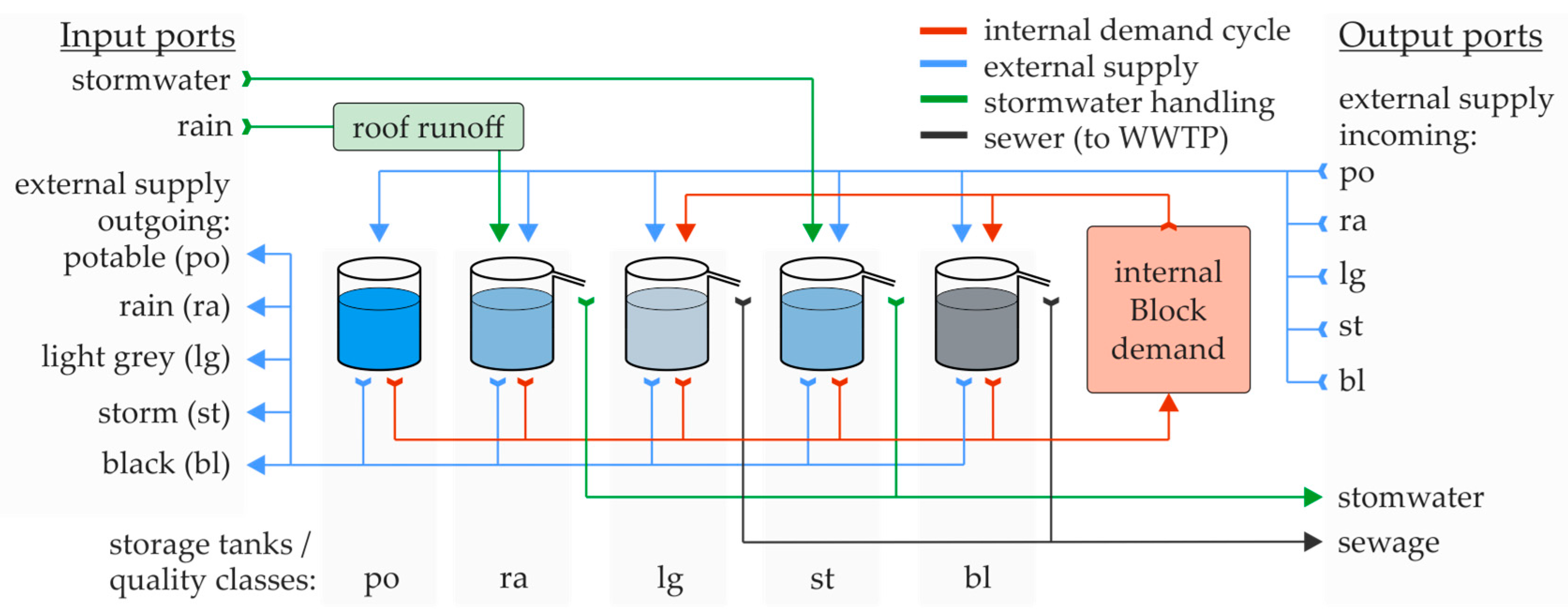
Figure 6.
Scheme of a WBM-Block; storage facilities for every QC as core of the Block, demand inside the Block, internal flow pathways and connections to the model environment.
Figure 6.
Scheme of a WBM-Block; storage facilities for every QC as core of the Block, demand inside the Block, internal flow pathways and connections to the model environment.
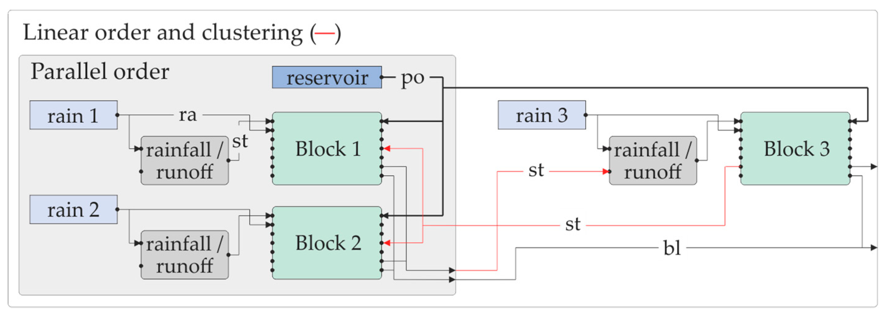
Figure 7.
Block connections in linear and parallel order, rain 1 to 3 is the regional precipitation for each Block, Block 1 and 2 are connected to the reservoir without connection to each other (parallel order), Block 3 serves as stormwater cluster; the input and output ports are ordered like shown in
Figure 6.
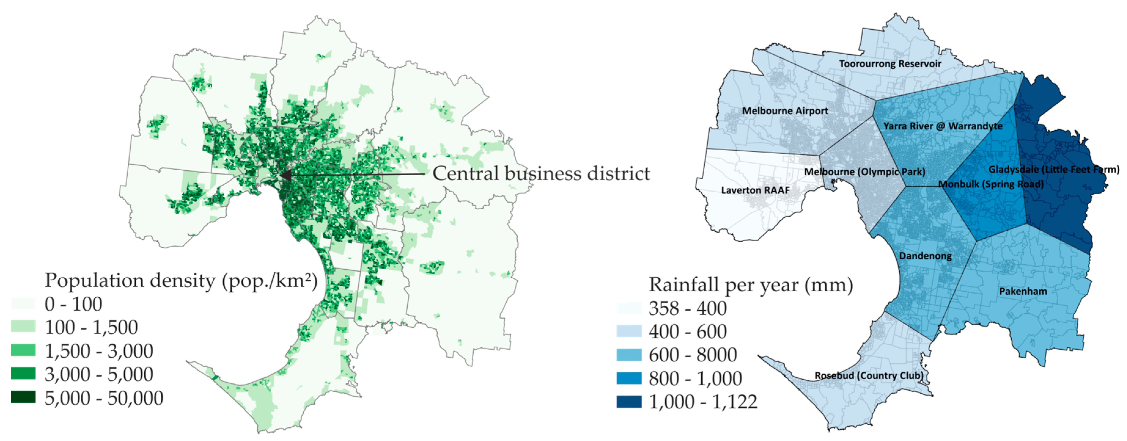
Figure 8.
Melbourne: population density (left); and rain distribution in mm/year (right).
Figure 8.
Melbourne: population density (left); and rain distribution in mm/year (right).
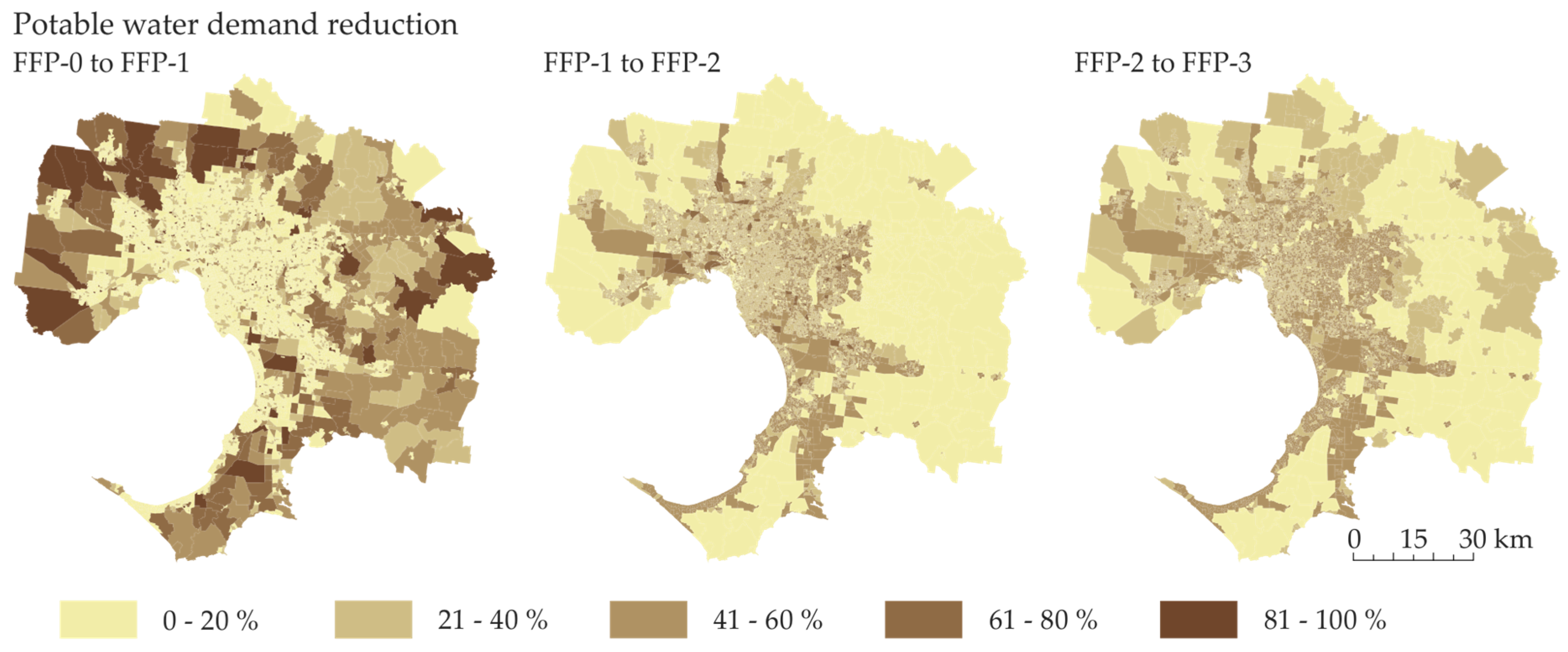
Figure 9.
Spatial analysis of the differences in annual potable water demand between FFP-0 to FFP-3.
Figure 9.
Spatial analysis of the differences in annual potable water demand between FFP-0 to FFP-3.
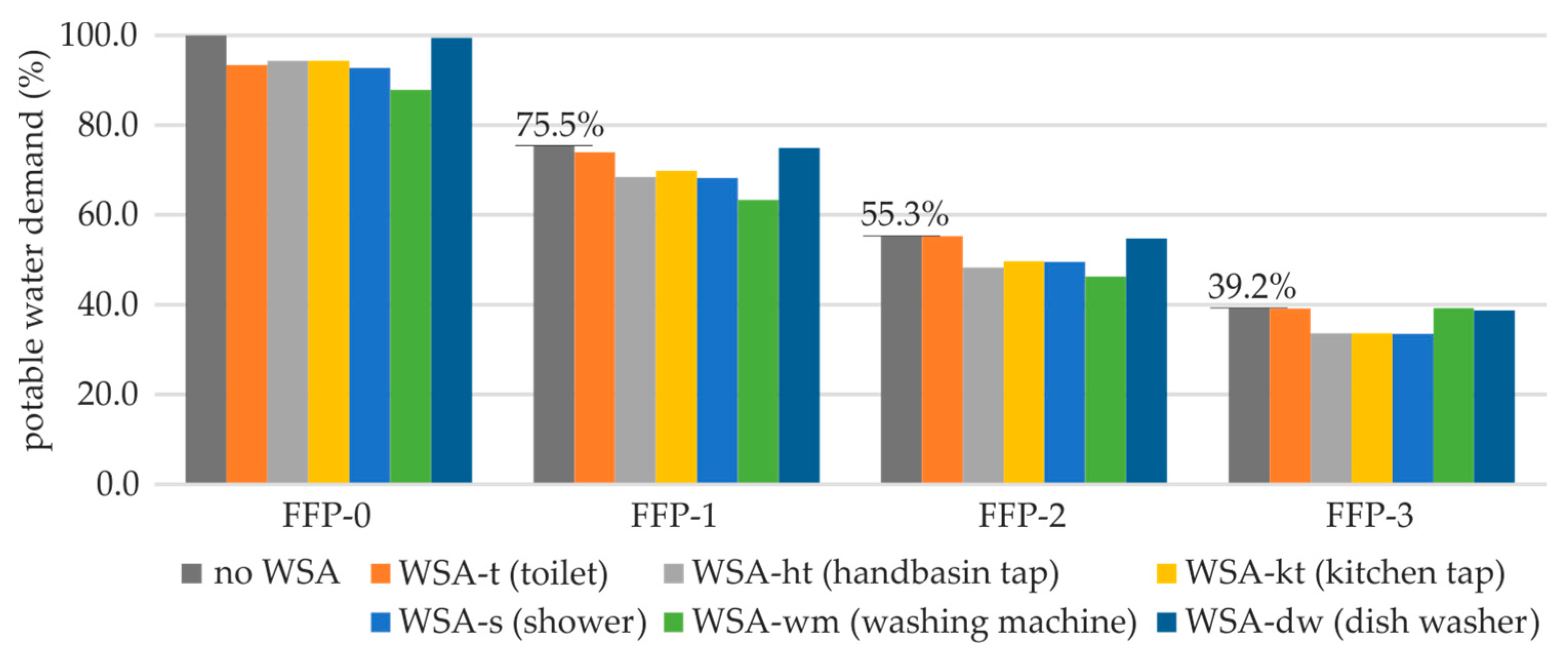
Figure 10.
Combination of the water saving appliances scenarios (WSA scenarios) and the FFP-policies. Annual potable water demand compared to the initial model without water saving appliances and with ffp-0 qualities. Each column represents the potable water demand of one WSA/FFP combination.
Figure 10.
Combination of the water saving appliances scenarios (WSA scenarios) and the FFP-policies. Annual potable water demand compared to the initial model without water saving appliances and with ffp-0 qualities. Each column represents the potable water demand of one WSA/FFP combination.
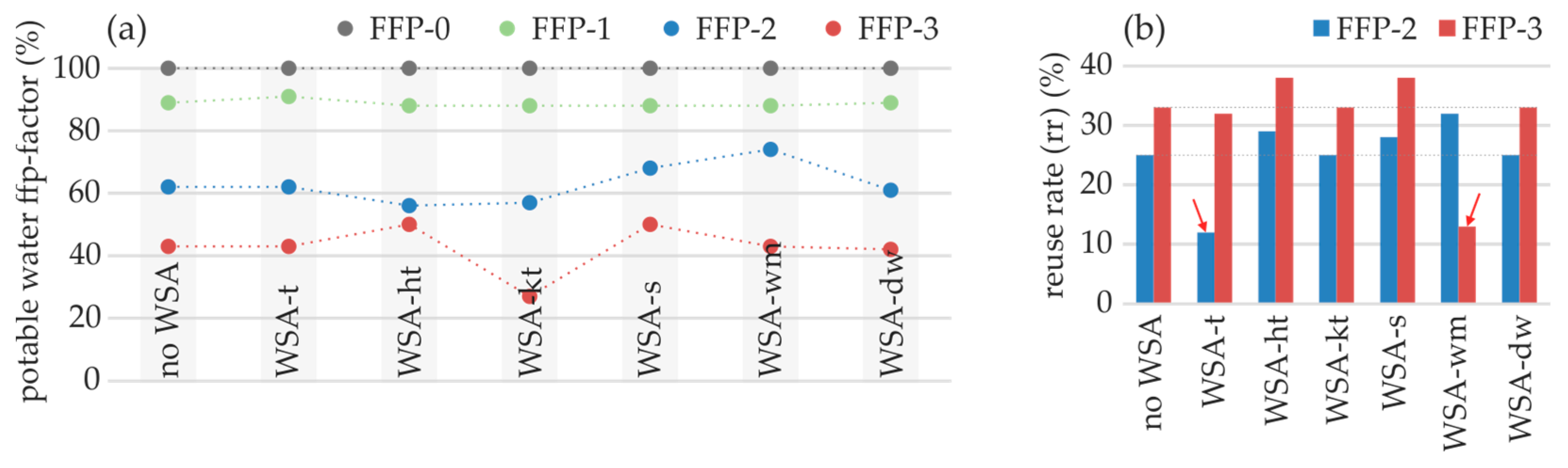
Figure 11.
Results from the WSA-scenarios: (a) the potable water ffp-factor (part of the demand that must be potable according to the definition); and (b) the greywater reuse rate (rr) (%).
Figure 11.
Results from the WSA-scenarios: (a) the potable water ffp-factor (part of the demand that must be potable according to the definition); and (b) the greywater reuse rate (rr) (%).
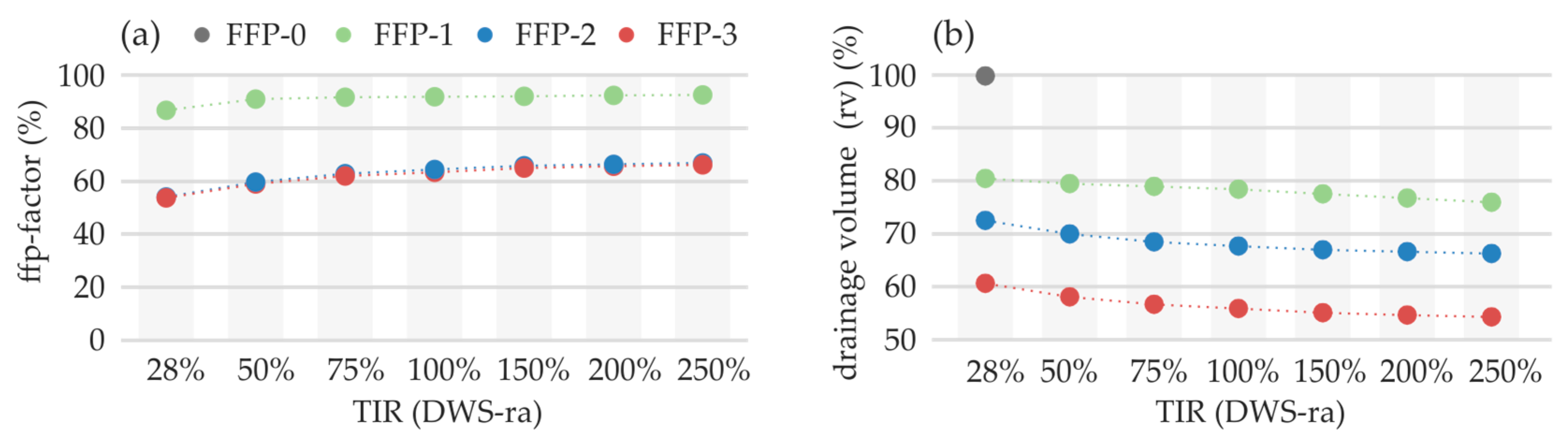
Figure 12.
Results from the DWS-ra scenarios (combined with FFP-1 to FFP-3): (a) ffp-factor (defined rainwater demand covered by ra); and (b) annual drainage volume (rv) (FFP-0 as reference runoff).
Figure 12.
Results from the DWS-ra scenarios (combined with FFP-1 to FFP-3): (a) ffp-factor (defined rainwater demand covered by ra); and (b) annual drainage volume (rv) (FFP-0 as reference runoff).
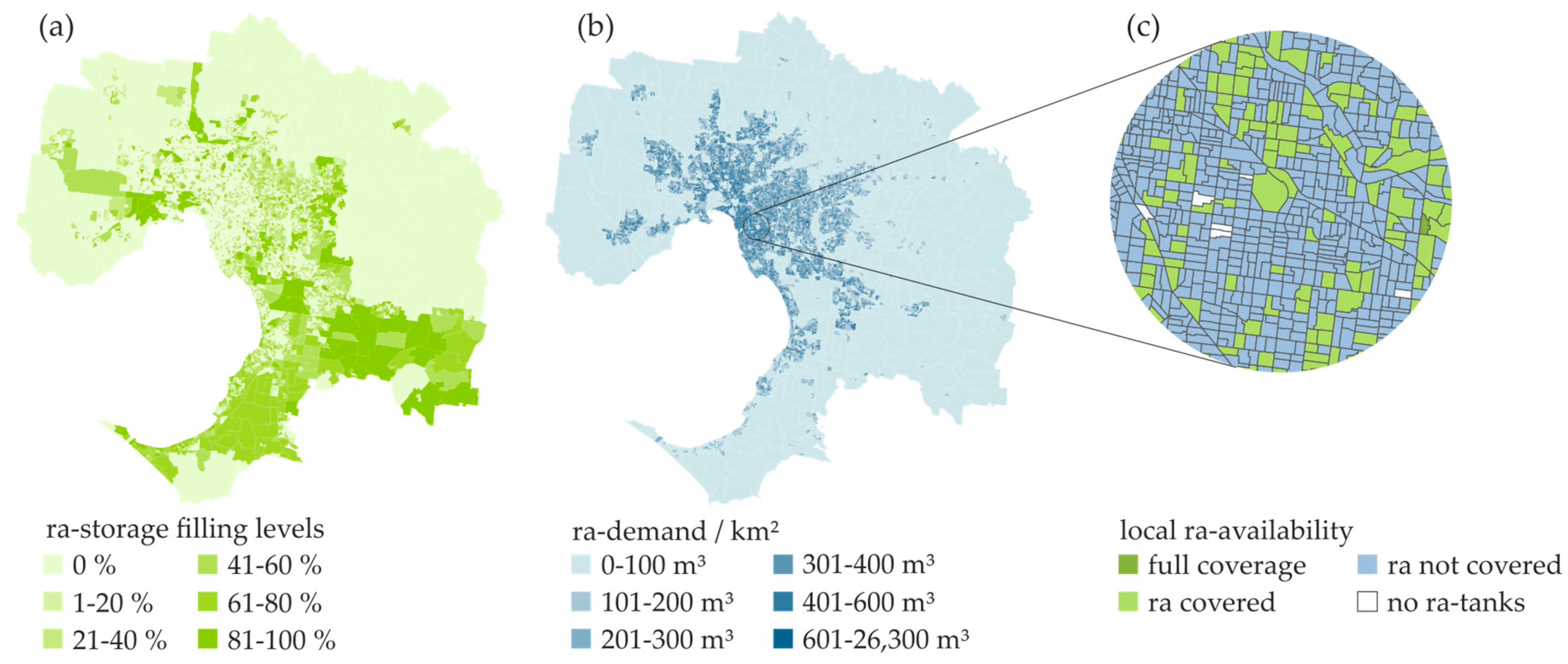
Figure 13.
Local difference in rainwater availability. Results from the DWS-ra (TIR 250%, FFP-3) for one summer day (15 December 2015): (a) fl for ra-storages (average of the day); (b) ra-demand in m3/km² (the highest demand value is caused by very small Block sizes); and (c) local disparity between Blocks where ra demand was met and where a QC-upgrade is necessary.
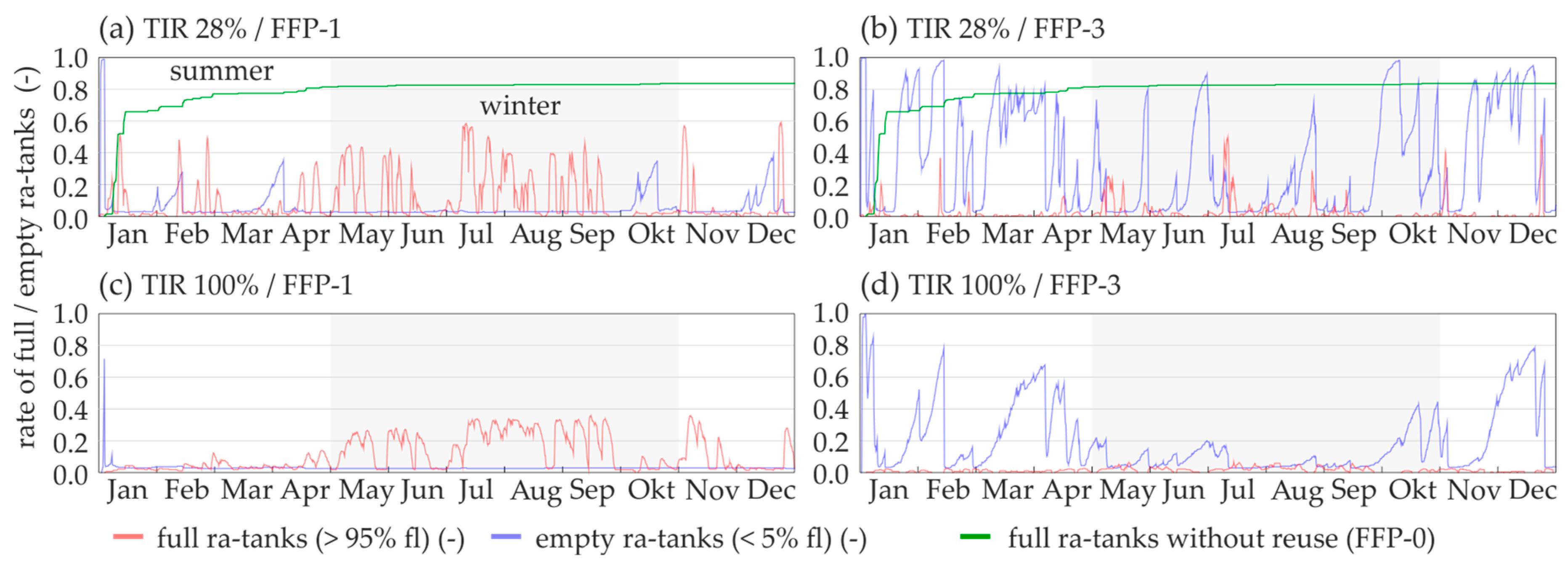
Figure 14.
Ratio of full and empty ra-tanks at each time step (DWS-ra): (a) TIR 28%, FFP-1; (b) TIR 28%, FFP-3; (c) TIR 100%, FFP-1; (d) TIR 100%, FFP-3; compared to the FFP-0 scenario (green line).
Figure 14.
Ratio of full and empty ra-tanks at each time step (DWS-ra): (a) TIR 28%, FFP-1; (b) TIR 28%, FFP-3; (c) TIR 100%, FFP-1; (d) TIR 100%, FFP-3; compared to the FFP-0 scenario (green line).
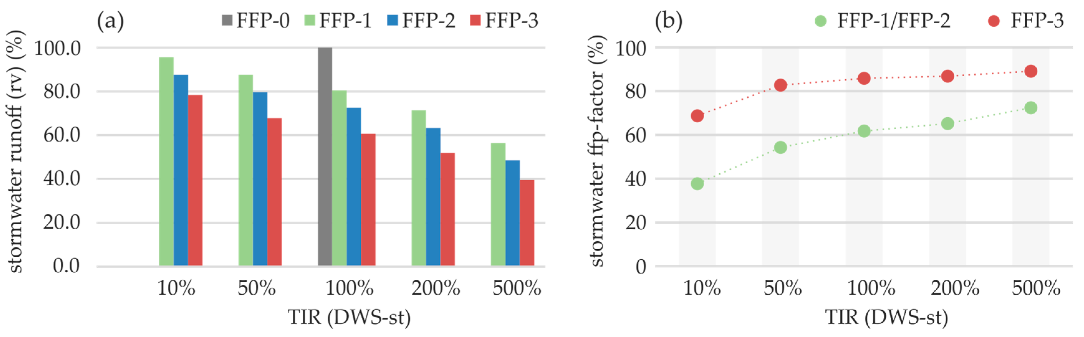
Figure 15.
Results for the DWS-st scenarios: (a) annual stormwater runoff volume (rv) compared to the FFP-0 without stormwater reuse; and (b) stormwater ffp-factor.
Figure 15.
Results for the DWS-st scenarios: (a) annual stormwater runoff volume (rv) compared to the FFP-0 without stormwater reuse; and (b) stormwater ffp-factor.
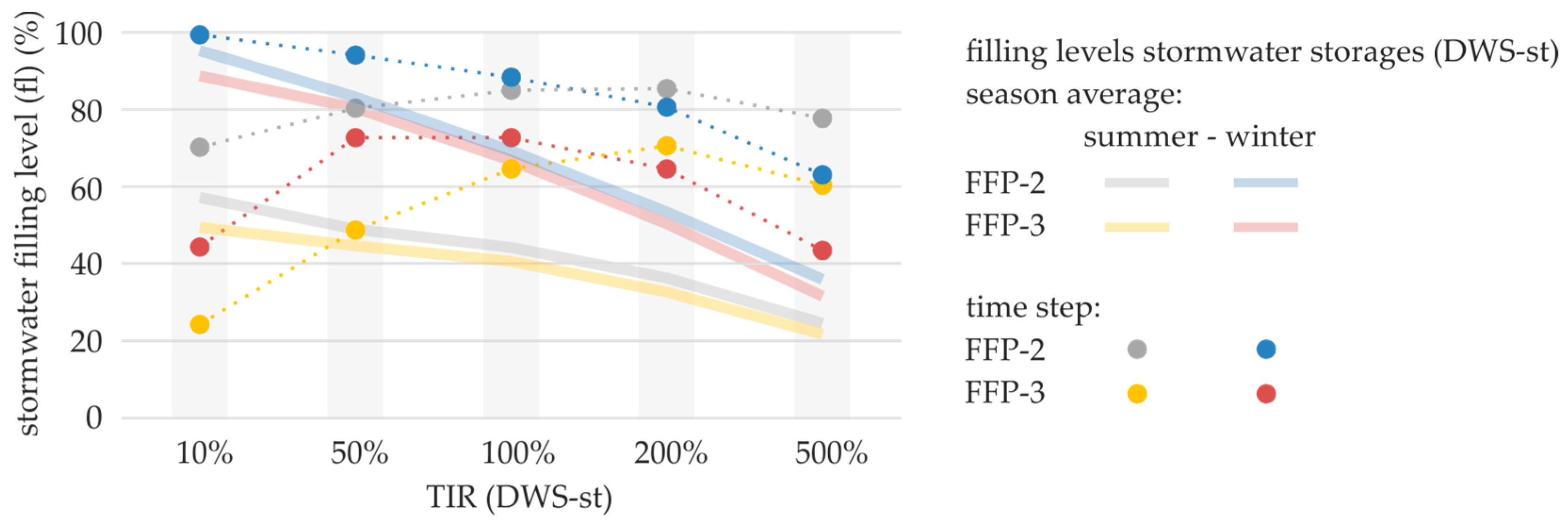
Figure 16.
Results for the DWS-st scenarios: filling levels (fl) of all storages for seasonal average and one time step (summer, 15 December 2015; winter, 1 July 2015; no rainfall for at least three days before measurement).
Figure 16.
Results for the DWS-st scenarios: filling levels (fl) of all storages for seasonal average and one time step (summer, 15 December 2015; winter, 1 July 2015; no rainfall for at least three days before measurement).
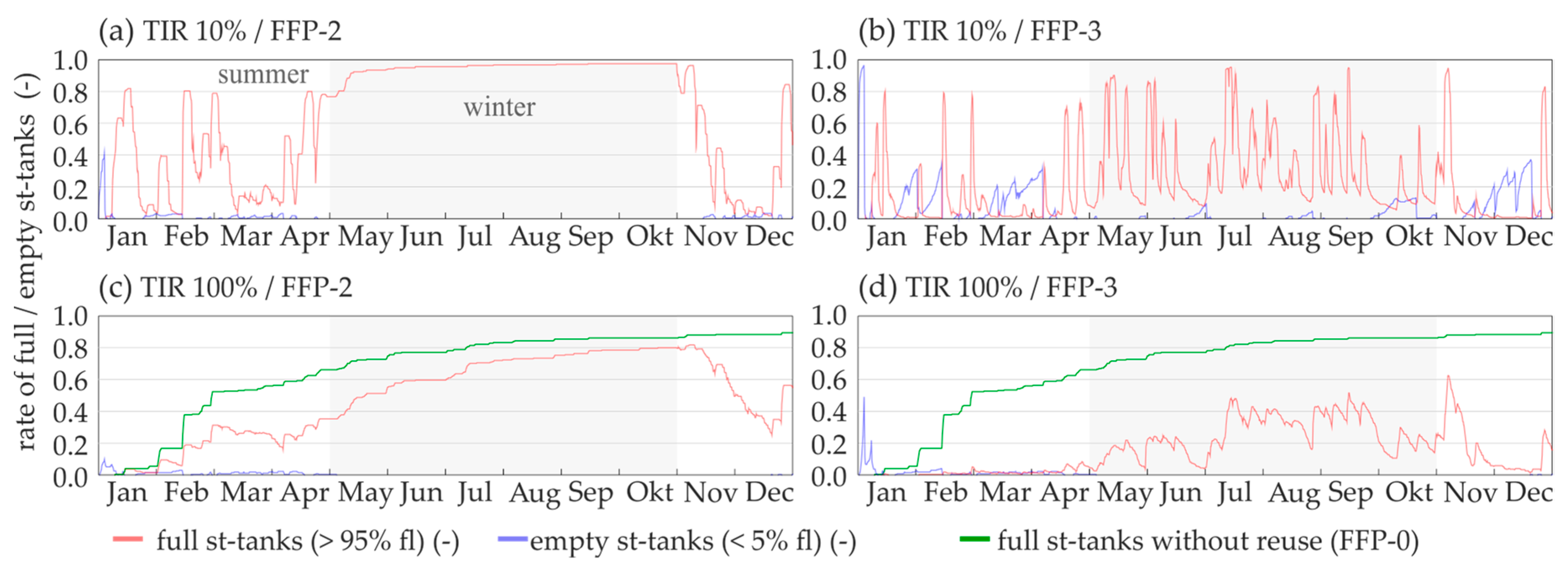
Figure 17.
Ratio of full and empty st-tanks at each time step (DWS-st): (a) TIR 10%, FFP-2; (b) TIR 10%, FFP-3; (c) TIR 100%, FFP-2; (d) TIR 100%, FFP-3.
Figure 17.
Ratio of full and empty st-tanks at each time step (DWS-st): (a) TIR 10%, FFP-2; (b) TIR 10%, FFP-3; (c) TIR 100%, FFP-2; (d) TIR 100%, FFP-3.
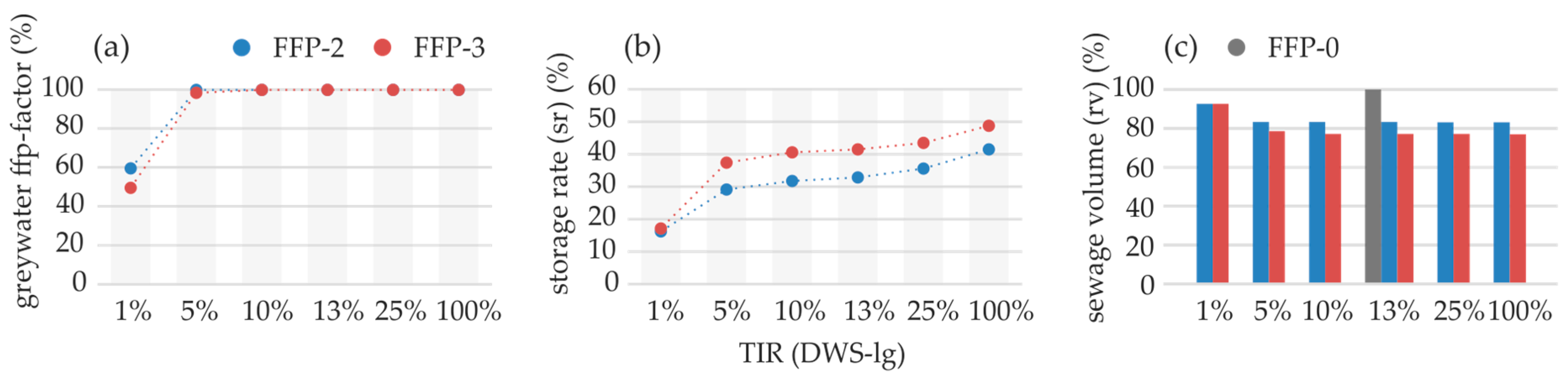
Figure 18.
Results for the DWS-lg scenarios: (a) ffp-factor for greywater; (b) greywater storage rate (sr); and (c) sewage volume (rv) compared to FFP-0 (without greywater reuse).
Figure 18.
Results for the DWS-lg scenarios: (a) ffp-factor for greywater; (b) greywater storage rate (sr); and (c) sewage volume (rv) compared to FFP-0 (without greywater reuse).
Table 1.
Example for water quality assignment to end-uses (in: demand/inflow; out: outflow after use).
Table 1.
Example for water quality assignment to end-uses (in: demand/inflow; out: outflow after use).
| Application | Assignment 1 | Assignment 2 |
|---|
| | in | out | in | out |
|---|
| Toilet | potable water | Black water | rainwater | Black water |
| Shower | potable water | Black water | potable water | light greywater |
| Irrigation | rainwater | - | stormwater | - |
Table 2.
Example for a water demand database of 1 specific water quality assignment, with curve scale of 500 people.
Table 2.
Example for a water demand database of 1 specific water quality assignment, with curve scale of 500 people.
| Scale | | Residents/Households | | Demand | | Outflow | | Number of DC’s |
|---|
| 500 | | 1–6 | | 5 QCs | | 2 QCs | | |
| | | | | 2 seasons | | 2 seasons | | |
| | | | | 1 + 7 WSA | | 1 + 7 WSA | | |
| 1 | × | 6 | × | (80 | + | 32) | = | 672 |
Table 3.
Input and output ports of a WB-Block.
Table 3.
Input and output ports of a WB-Block.
| Input Ports | Description | Output Ports | Description |
|---|
| Stormwater: | stormwater from rainfall/runoff module plus stormwater from the upstream Blocks | Stormwater: | combined stormwater and rainwater overflow |
| Rain: | rainfall of the current time step | Sewage: | combined grey and black water overflow |
| External supply: | claims from upstream Blocks | External supply: | required water to cover the storages |
Table 4.
Overview of the evaluated scenarios and the number of combinations.
Table 4.
Overview of the evaluated scenarios and the number of combinations.
| Scenario Overview | ID | Number of Scenarios | Scenario Combination |
|---|
| Quality requirements: | FFP-0/FFP-1 to FFP-3 | ![Sustainability 10 00716 i001]() | 4 |
| Water infrastructure scenarios: | | |
| water saving appliances | WSA-scenarios | 24 |
| decentralised water storages | DWS-scenarios | 9 |
| | | | 37 |
Table 5.
Water quality assignment scenarios (in: demand/inflow; out: outflow after usage).
Table 5.
Water quality assignment scenarios (in: demand/inflow; out: outflow after usage).
| Application | FFP-0 (ref) | FFP-1 | FFP-2 | FFP-3 |
|---|
| | in | out | in | out | in | out | in | out |
|---|
| Toilet | po | bl | ra | bl | lg | bl | st | bl |
| Hand basin tap | po | bl | po | bl | po | lg | ra | lg |
| Kitchen tap | po | bl | po | bl | po | bl | po | bl |
| Bath | po | bl | po | bl | po | lg | ra | lg |
| Shower | po | bl | po | bl | ra | lg | ra | lg |
| Washing machine | po | bl | po | bl | ra | lg | lg | lg |
| Dish washer | po | bl | po | bl | po | bl | po | bl |
| Private irrigation | po | - | ra | - | lg | - | st | - |
| Public irrigation | po | - | st | - | st | - | st | - |
| Farm Irrigation | po | - | st | - | st | - | st | - |
Table 6.
Water saving appliances (WSA) scenarios.
Table 6.
Water saving appliances (WSA) scenarios.
| Appliance | “6-Star” Water Saving Appliances | Adaption Ratio |
|---|
| Toilet (WSA-t) | 2.5 L/flush | 0.445 |
| Hand basin tap (WSA_ht) | 1.1–4.5 (2.8) L/min | 0.518 |
| Kitchen tap (WSA-kt) | 1.1–4.5 (4.5) L/min | 0.328 |
| Bath | - | 1.0 |
| Shower (WSA-s) | 4.5 L/min | 0.614 |
| Washing machine (WSA-wm) | 30.3 L/load (6 kg) | 0.254 |
| Dish washer (WSA-dw) | 8.3 L/event (12 place settings) | 0.572 |
Table 7.
Decentralised water storage (DWS) scenarios.
Table 7.
Decentralised water storage (DWS) scenarios.
| Storage Tank | Design Parameter | TIR |
|---|
| Rainwater (DWS-ra) | Households | 28 to 250% |
| Stormwater (DWS-st) | Block size | 0 to 500% |
| Greywater (DWS-lg) | Residents | 0 to 100% |
Table 8.
Performance indicators.
Table 8.
Performance indicators.
| Performance Indicator | Description |
|---|
| Demand (td) [%] | Demand for each water quality class in percent compared to the total demand |
| Runoff volume (rv) [%] | Stormwater/sewage runoff and runoff peaks compared to the initial model |
| Filling levels (fl) [%] | The filling level compared to the tank volume, available for every storage in the model. This indicator shows the availability of resources all over the investigation area. |
| Fit-for-purpose factor (ffp-factor) [%] | The ffp-factor symbolises the percentage of a QC’s demand, which is not upgraded and met by the intended QC.
In the case of potable water, no upgrade is possible, so the ffp-factor is turned to represent the ratio of the used potable water that must be potable by definition. (Not to be confused with the FFP-policies, which are used for scenario identification) |
| Reuse rate (rr) [%] | This indicator represents the percentage of greywater that is used again (calculated as greywater use/greywater generation) |
| Storage rate (sr) [%] | The percentage of generated greywater that is stored in the tanks (calculated as stored greywater/greywater generation) |
Table 9.
Annual results for water demand, sewage and stormwater runoff and the performance indicator “ffp-factor”. Reference scenario (FFP-0) is taken as 100%, FFP-1 to FFP-3 quality assignment compared to the FFP-0 (for this simulation the initial model is used).
Table 9.
Annual results for water demand, sewage and stormwater runoff and the performance indicator “ffp-factor”. Reference scenario (FFP-0) is taken as 100%, FFP-1 to FFP-3 quality assignment compared to the FFP-0 (for this simulation the initial model is used).
| | | FFP-0 (Reference) | FFP-1
(%) | FFP-2
(%) | FFP-3
(%) |
|---|
| Demand (td) | po | 4.230 × 10⁸ m3/year * | 100% | 75.5 | 55.3 | 39.2 |
| ra | - | - | 10.6 | 18.3 | 18.4 |
| lg | - | - | - | 12.4 | 16.9 |
| st | - | - | 14.0 | 14.0 | 25.4 |
| Sewage (ss) | Volume | 3.141 × 10⁸ m3/year | 100% | 100.0 | 83.3 | 77.2 |
| Peak | 7.416 × 10⁴ m3/h | 100% | 100.0 | 83.8 | 86.5 |
| Stormwater (ss) | Volume | 3.957 × 10⁶ m3/year | 100% | 80.5 | 72.5 | 60.6 |
| Peak | 9.898 × 10⁵ m3/h | 100% | 85.5 | 84.1 | 76.8 |
| ffp-factor | po | 1.0 | 100% | 89.1 | 61.8 | 42.7 |
| re | - | - | 87.0 | 54.0 | 53.0 |
| lg | - | - | - | 99.0 | 99.0 |
| st | - | - | 62.0 | 62.0 | 86.0 |
Table 10.
Annual potable water demand for the rainwater storage scenarios (DWS-ra).
Table 10.
Annual potable water demand for the rainwater storage scenarios (DWS-ra).
| TIR: | 28% | 50% | 75% | 100% | 150% | 200% | 250% |
|---|
| (DWS-ra) | (initial model) | | | | | | |
| FFP-1 | 3.192 × 10⁸ m3 | 99.2% | 99.1% | 99.0% | 98.9% | 98.9% | 98.8% |
| FFP-2 | 2.339 × 10⁸ m3 | 96.3% | 94.2% | 93.1% | 92.1% | 91.8% | 91.5% |
| FFP-3 | 1.659 × 10⁸ m3 | 94.9% | 91.9% | 90.4% | 88.7% | 87.9% | 87.4% |
Table 11.
Annual potable water demand for the stormwater storage scenarios (DWS-st).
Table 11.
Annual potable water demand for the stormwater storage scenarios (DWS-st).
| TIR: | 10% | 50% | 100% | 200% | 300% | 400% | 500% |
|---|
| (DWS-st) | | | (initial model) | | | | |
| FFP-1 | 108.2% | 103.1% | 3.192 × 10⁸ m3 | 98.3% | 97.6% | 96.6% | 95.9% |
| FFP-2 | 112.0% | 104.2% | 2.339 × 10⁸ m3 | 97.8% | 96.6% | 95.4% | 94.4% |
| FFP-3 | 115.8% | 106.0% | 1.659 × 10⁸ m3 | 96.8% | 95.1% | 93.5% | 92.0% |
Table 12.
Annual potable water demand for greywater storage scenarios (DWS-lg), greywater is only used for FFP-2 and FFP-3.
Table 12.
Annual potable water demand for greywater storage scenarios (DWS-lg), greywater is only used for FFP-2 and FFP-3.
| TIR | 1% | 5% | 13% | 25% | 100% |
|---|
| (DWS-lg) | | | initial model | | |
| FFP-2 | 110.70 | 100.10 | 2.339 × 10⁸ m3 | 99.97 | 99.88 |
| FFP-3 | 125.09 | 102.18 | 1.659 × 10⁸ m3 | 99.93 | 99.75 |

 ,
, 


