Article

Modeling the Impacts of Conservation Agriculture with a Drip Irrigation System on the Hydrology and Water Management in Sub-Saharan Africa

1
Faculty of Civil and Water Resource Engineering, Institute of Technology, Bahir Dar University, Bahir Dar 26, Ethiopia
2
Department of Civil, Architectural and Environmental Engineering, North Carolina A&T State University, Greensboro, NC 27411, USA
3
Sustainable Intensification Innovation Lab (SIIL), Kansas State University, Manhattan, KS 66506, USA
4
Texas A&M AgriLife Research, Temple, TX 76502, USA
*
Author to whom correspondence should be addressed.
Sustainability 2018, 10(12), 4763; https://doi.org/10.3390/su10124763
Submission received: 4 August 2018 / Revised: 25 November 2018 / Accepted: 2 December 2018 / Published: 13 December 2018

Abstract

:
The agricultural system in Sub-Saharan Africa (SSA) is dominated by traditional farming practices with poor soil and water management, which contributes to soil degradation and low crop productivity. This study integrated field experiments and a field-scale biophysical model (Agricultural Policy Environmental Extender, APEX) to investigate the impacts of conservation agriculture (CA) with a drip irrigation system on the hydrology and water management as compared to the conventional tillage (CT) practice. Field data were collected from four study sites; Dangishita and Robit (Ethiopia), Yemu (Ghana), and Mkindo (Tanzania) to validate APEX for hydrology and crop yield simulation. Each study site consisted of 100 m2 plots divided equally between CA and CT practices and both had a drip irrigation setup. Cropping pattern, management practices, and irrigation scheduling were monitored for each experimental plot. Significant water savings (α = 0.05) were observed under CA practice; evapotranspiration and runoff were reduced by up to 49% and 62%, respectively, whereas percolation increased up to three-fold. Consequently, irrigation water need was reduced in CA plots by about 14–35% for various crops. CA coupled with drip irrigation was found to be an efficient water saving technology and has substantial potential to sustain and intensify crop production in the region.

1. Introduction

Agricultural production continues to face several challenges in Sub-Saharan Africa (SSA) leading to an insufficient food supply. The population significantly increased from 180 million to 962 million from 1950 to 2015 in SSA [1]. This rapid increase in population imposes a pressure on the already stressed food production system. Insufficient food supply leads to malnutrition, which accounts for more than one-third of all children’s death in the region [2]. Another challenge is the rainfall-dependent farming system, which makes it susceptible to climate variability such as drought [3]. Also, the expansion of traditional farming practices aiming to increase in food supply resulted in environmental deterioration due to conventional tillage practices [4,5]. These challenges call for a sustainable growth in food production system that may come from (1) growing high value and nutritious food types, such as fruits and vegetables; (2) using efficient water use strategies (irrigation technologies) that can maximize production and support multiple cropping seasons; (3) enabling dry season cropping (climate resilient system) through water storage; and (4) disseminating best management practices through field demonstrations and other educational and outreach activities. The focus should be to empower smallholder farmers, which constitutes the majority of farms (80%) in SSA [6].
Home gardens (a concept of producing fruits and vegetables closer to the household) conceptually provide both food and nutrition, and may potentially serve as a source of income to smallholder farmers. If the majority of the yields can be sold, the system can be called commercial home gardens (CHGs) [7]. CHGs provide incentives for farmers and balanced diets as they use part of the production for household consumption. The concept can be applied in any farming system including the conventional tillage (CT) system. However, the benefits can be enhanced sustainably if it can be combined with a conservation agriculture (CA) system [8], which has been proven to be a very efficient system as it promotes better soil and water management strategies. CA is a sustainable agricultural system that provides higher production efficiency, water savings, and environmental protection [9,10,11,12]. Moreover, including an efficient water application technology would have significant potential to maximize water use efficiency and thus increase food production and conserve the environment. Drip irrigation is an efficient water application technology, which provides uniform water supply and minimum soil disturbance during irrigation. Several studies, including References [13,14,15,16,17], verified the system as being a highly efficient and sustainable water application technique.
This study aimed to examine and demonstrate the usefulness of the CA system over traditional CT systems in CHGs using both field-experiments and a modeling study. Both systems were implemented under drip irrigation technology for efficient water application. CA refers to (1) minimized soil disturbance (no-till), (2) continuous organic mulch covers on the soil surface, and (3) diverse cropping in the rotation. In contrast, CT refers to the traditional farming practice using conventional tillage operations with no mulch application. Combining CA and drip irrigation in CVHGs is an ideal approach to maximize agricultural water savings further. Despite several benefits of CA and drip irrigation systems individually, very little is known about their combined effects on water management for vegetable production in SSA.
Field-scale experimental studies are essential; however, they are mostly limited to certain variable records for a short period. This makes the evaluation of soil and water management technology difficult without the help of modeling techniques. Modeling techniques are essential to evaluate the impacts of soil and water management practices beyond the measured variables and to understand the underlying processes better. The choice of an appropriate model is vital to provide reliable evidence. Recent advances in biophysical models would help to evaluate the effects of management practices at various spatial and temporal scales [18,19,20,21,22,23,24]. Watershed models are mainly developed considering specific site conditions, and may or may not perform well for other regions [25,26]. Thus, verifying a watershed model for a region is necessary to ensure the reliability of model results. The performance of a model is directly related to the representation of underlying processes [27]. The lack of detailed field data is usually a constraint to verify a model performance [26,28,29]. Agricultural Policy Environmental Extender (APEX) [30,31,32,33,34] is among the few efficiently tested, process-based watershed models. APEX is capable of evaluating the effects of various water and land management practices on watershed hydrology and water quality at various spatiotemporal scales [35,36]. This study evaluates the effects of CA with drip irrigation on hydrological process and water management using the APEX model. Experimental data from field sites in all four locations were used to parameterize the model for calibration and validation.

2. Materials and Methods

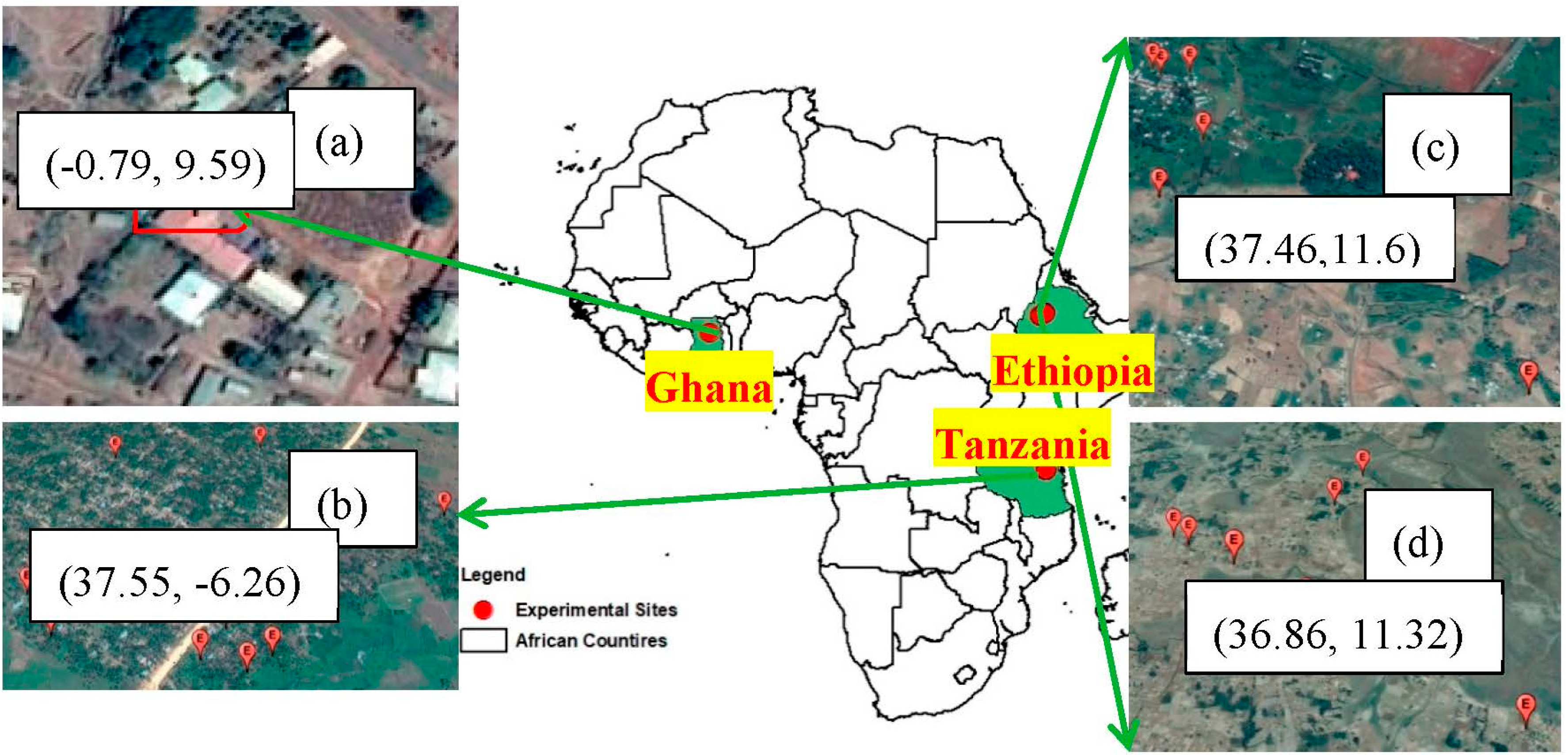
2.1. Site Description

This study was conducted at four experimental sites in Sub-Saharan Africa. Dangishita and Robit sites were in northern Ethiopia, whereas Yemu and Mkindo were in the north and southeast of Ghana and Tanzania, respectively (Figure 1). A total of 43 experimental plots (Robit—6 plots, Dangishita—7 plots, Yemu—15 plots, and Mkindo—15 plots) were established on a 100 m2 (paired “t” design), in which half of this site was assigned randomly to CA and another half to CT (Figure 2). Low-cost drip irrigation was installed for both cases. Simple water-lifting technologies were introduced to extract water from groundwater wells and deliver it into water storage tanks (usually 500 L in size). Irrigation water was distributed to the fields using gravity flow from these tanks, installed about 1.5 m above the ground. Farmers could use their intrinsic knowledge to decide the frequency of irrigation (i.e., depending on vegetable water need and on-site observation of soil moisture). Dangishita and Robit sites were situated on Chromic Luvisols soil (hydrologic group C) whereas Yemu and Mkindo sites were on Ferric Luvisols soil (hydrologic group A) and Ferallic Cambisols soil (hydrologic group D), respectively. The infiltration and water transmission rate decrease from hydrologic soil group A to D. Table 1 shows detailed soil characteristics of experimental sites derived using a soil-plant-atmosphere-water (SPAW) field and pond hydrology program. Inputs for the SPAW hydrology program were provided from a harmonized world soil database [37].
Watershed and plot level parametrization were made for Dangishita, whereas plot level parametrization was made for the other sites (due to streamflow data limitation). Streamflow gauging station records in Dangishita were used to verify APEX model simulation at the watershed scale. Figure 3 shows the Dangishita watershed extracted from a 30 m resolution digital elevation model at the outlet, which had a streamflow gauging station, and the experimental plots were close to the watershed outlet. The size of Dangishita watershed was 57.5 km2 and the majority of the landscape, about 80%, was had less than a 10% slope. Climatic data for the study sites were obtained from nearby weather stations (Dangila for Dangishita sites; and Bahir Dar for Robit sites) (Figure 3) and nearby climate forecast system reanalysis (CFSR) data for Yemu (Ghana) and Mkindo (Tanzania) due to lack of ground weather data close to the study sites. The CFSR data for Yemu (1980–2013) and Mkindo (1980–2010) obtained from Texas A&M was bias-corrected with a linear bias correction as indicated in Reference [38]. The mean monthly rainfall of the study sites for Dangishita and Robit (2010–2016) and Yemu and Mkindo (2010–2014) are shown in Figure 4. The mean annual rainfall was found to be 1711 mm and 1394 mm (2010–2016) for Dangishita and Robit, respectively, and 1012 mm and 948 mm (2010–2014) for the Yemu and Mkindo sites, respectively.

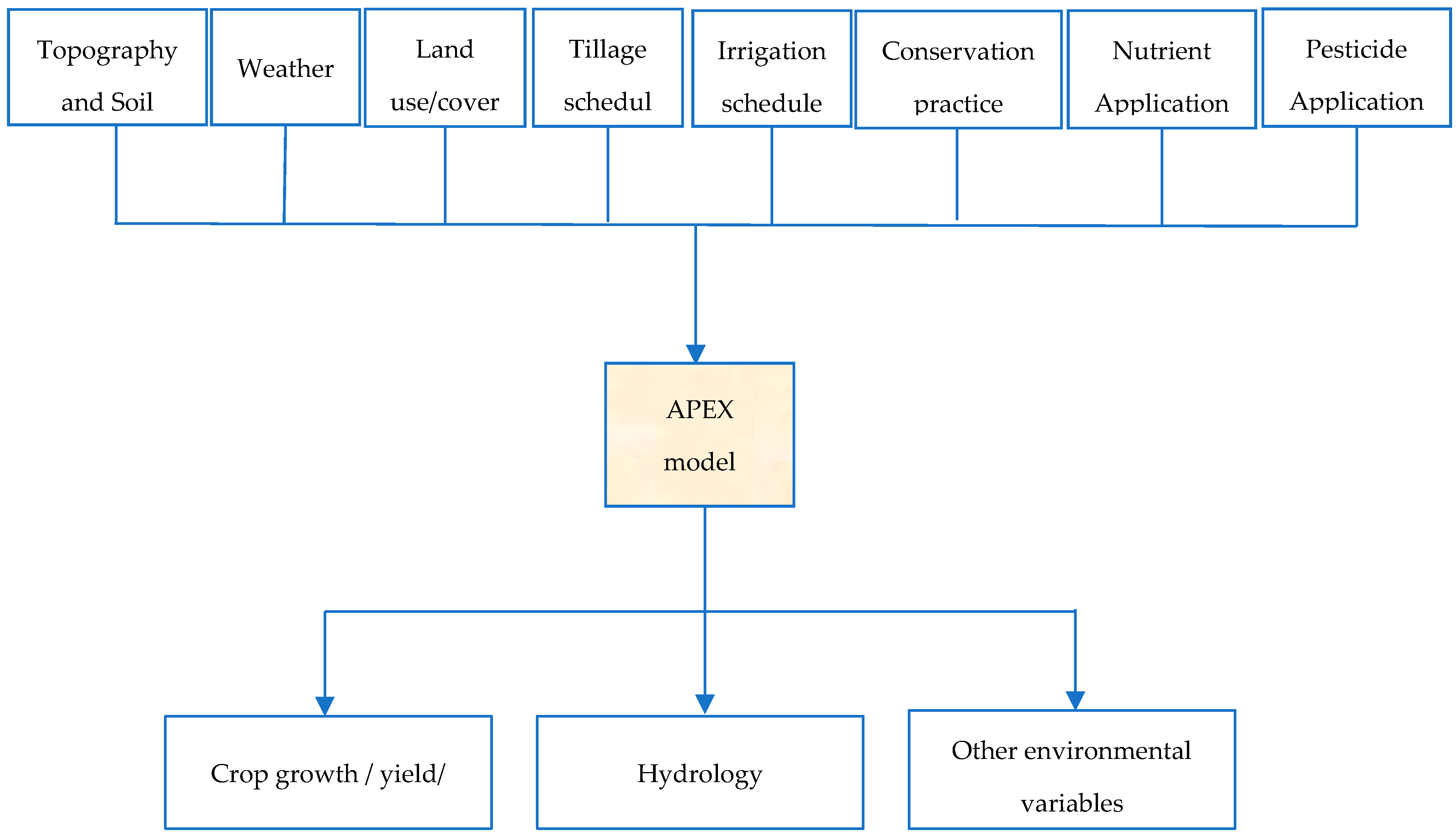
2.2. APEX Model Description, Inputs, and Data Monitoring

APEX is an extension of the Environmental Policy Integrated Climate (EPIC) model [39]. APEX, a biophysical model [39], is capable of evaluating the effects of various soil and water management practices on the hydrology of the system, crop growth, and other environmental factors [40]. It has the capability of modeling wide ranges of conservation practices [23,35,41,42,43,44]. APEX simulates watershed processes based on weather data, soils characteristics, topography, vegetation, and management practices [40]. Multiple options are available in the APEX model to estimate evapotranspiration, surface runoff, peak runoff rate, and available soil water capacity to derive hydrology of the system [45]. Recently, the “ADDMULCH” management was included in the APEX model (2017 release) to simulate organic mulch cover conservation practices on the soil surface. Detailed description of the APEX model major components (Figure 5) can be found in Reference [46]. The APEX model has been applied to evaluate the effects of conservation practices [35,41,43,44].
The APEX model inputs include Geographic Information System (GIS) data layers, climatic data, and management practices. The GIS data layers are digital elevation model, soil and land use or crop covers. A 30 m digital elevation model (DEM) was obtained from the United States Geographical Survey (USGS) website and used to extract watershed characteristics. Soil map prepared by the Ministry of Water, Irrigation and Energy (MoWIE) of Ethiopia were used for the Dangishita and Robit sites. A harmonized world soil map prepared by the Food and Agricultural Organization (FAO) were used for the case of Yemu and Mkindo. Ground climate stations were used for Dangishita and Robit sites, whereas bias-corrected CFSR data were used for Yemu and Mkindo sites. Various management activities and cropping patterns were monitored at each site. The management activities include tillage and planting details; population density; mulch application rate and date; fertilizer and pesticide details, irrigation application rate, and the amount and harvesting date. Groundwater wells were used in Dangishita and Robit sites as a source of drip irrigation, whereas surface water (river) was used for Yemu and Mkindo sites. Farmers used a manual pulley system to lift water from groundwater wells to a water tank. Farmers in Yemu used motorized pumps with pipes to deliver the water from the river pond to the water tanker, whereas farmers in Mkindo used a faucet (installed at their home) to fill the water tank. The sizes of the water tanks were 500 L (in Dangishita, Robit, and Mkindo) and 200 L (in Yemu), which were placed near vegetable gardens about one and a half meter above the ground. The water dripped from a storage tank to the plots until the tank was empty (i.e., fixed amount of water per single irrigation). Farmers decide the frequency of irrigation through field observation (i.e., by touching the soil using their hand and observing soil moisture). The date of irrigation application and the number of water tanks used were monitored. A management file was developed, which included irrigation the amount and date of application, and integrated into the model separately for (CA and CT management).

2.3. Model Setup and Prediction of Hydrology

APEX version 1501 (Texas A&M AgriLife Research, Temple, Texas, USA) was used for the model setup. A user-defined watershed with 50 m2 (each for CA and CT) and stream shapefiles were created to represent an experimental commercial vegetable home garden site. An ArcGIS interface, Arc-APEX (Texas A&M AgriLife Research, Temple, Texas, USA), was used to integrate user-defined vegetable garden, process GIS data layers, and input climatic data. Distinct farm-scale model setups (CA and CT) were carried out for each study site (Dangishita, Robit, Yemu, and Mkindo) which have different weather, topography, vegetation, and management activities. Also, the watershed-based model was established for Dangishita watershed depending on the location of streamflow gauging site. The first step in setting up the APEX model began with the processing of GIS data layers to delineate the watershed boundary, subareas, and derive watershed characteristics. Watershed characteristics for Dangishita watershed and experimental plots were derived from the Digital Elevation Model (DEM). The second step was to integrate weather data using the Arc-APEX model interface. Moreover, the third step was to perform an initial model run and complete model setup procedures to create APEX model output files for further analysis. All monitored management activities (Table 2) were integrated into the operation file. The “ADDMULCH” operation was recently included for APEX version 1501 (2017 release) in the fertilizer database to account for the impacts of adding organic mulch cover; input data required the application date and amount of mulch in kg ha−1. A fixed irrigation application rate (drip irrigation) was provided in the management files. APEX model outputs were updated by re-running the model with modified management files.
The APEX hydrology model simulates all the key water balance components of the system. Precipitation, snow melts, and irrigation are the main inputs to the system, which are then disseminated into various components: surface runoff, subsurface/tile drainage flow, soil water, percolation, and evapotranspiration [46]. The routing phase of hydrology includes the water balance and nutrients. In APEX, the key landscape processes we considered across hydrologically connected units called subareas [45]. Subareas are the smallest unit in APEX with homogenous watershed characteristics, such as soil types, land use/crop cover, slope, and management.
APEX provides two options to estimate the runoff volume [46]: the modified soil conservation service (SCS) [47] curve number (CN) and Green and Ampt infiltration [48] methods. The SCS-CN runoff estimate method (Equations (1a) and (1b)) is a function of rainfall and retention parameter (Equation (2)). CN is a function of land use, management practice, and hydrologic soil group. The subsurface flow is a function of the vertical and horizontal flow and simulated as a simultaneous process [45]. The horizontal flow consists of a lateral flow, whereas the vertical flow (percolation) adds to groundwater storage, which is then subjected to return flow or deep percolation. The vertical component of percolation is calculated as a function of soil water content, field capacity, and travel time (Equation (3)). Five options are available to estimate the potential evapotranspiration: Penman, Penman–Monteith, Baier and Robertson, Priestly and Taylor, and Hargreaves methods [46]. The Hargreaves method is dynamic with a lower data requirement, and is a function of solar radiation, latent heat of vaporization, and temperature (Equation (4)). The methods for computing various hydrological components were selected based on the better simulation of variables before conducting a rigorous sensitivity calibration. The equations of each hydrological component and their descriptions can be found in Reference [39].
Q i = R i 0.2 S R i + 0.8 S ;   R > 0.2 S
Q i = 0.0 ;   R < 0.2 S
S = 254 ( 100 C N 1 )
P i = ( S W ( i ) F C ( i ) ) X 3 ( 1 + X 2 X 1 )
E T i = 0.0032 ( R A M X i H V ) ( T X + 17.8 ) ( T M X i T M N i ) 0.6
where Qi, Ri, ETi, Pi, S, CN, RMXi, HV, SW, FCi, TX, TMXi, TMNi, are runoff, precipitation, evapotranspiration, percolation, return flow, retention parameter, curve number (no unit), maximum daily solar radiation at mid-month (MJ/m2/d), latent heat of vaporization (MJ/kg), soil water, field capacity, average, and minimum and maximum temperature (°C) on day i, respectively. All other unspecified units are in mm. X1, X2, and X3 are travel functions of vertical, horizontal, and both vertical and horizontal travel time.

2.4. The “ADDMULCH” Subroutine

The new subroutine named “ADDMULCH” was developed and integrated in the APEX model to simulate the effect of adding organic mulch-cover on the soil surface. The subroutine adds the partial weight of the organic mulch (kg/ha) as carbon and nitrogen to the soil composition via two litter pools: metabolic and structural. Both pools receive equal amount of carbon (21% of the mulch weight) and nitrogen (0.42% of the mulch weight). Additionally, 3.7% of the weight as carbon and 0.35% of the weight as nitrogen are also added to the lignin component of the structural litter.

2.5. Sensitivity Analysis, Model Calibration, and Validation

Model sensitivity analysis is a method of identifying key parameters that affect model performance and are essential for model parametrization. The APEX model has large sets of parameters related to hydrology, sediment, nutrients, crops, and other environmental factors. Sensitivity analysis is the first step for hydrological models, which helps to diagnose and narrow down the large sets of parameters for calibration. Model calibration is a process in which model parameters are modified so that a model output mimics observed data, whereas validation is the use of modified parameters to simulate another set of observed data. The APEX auto-calibration and uncertainty estimator (APEX-CUTE) was used to perform sensitivity analysis and auto-calibration for the APEX hydrology model [40], followed by manual adjustment of a few parameters.
The first step was to examine the APEX hydrology model outputs for modifications. Some default methods and input parameters might need modification to get better simulation prior to sensitivity analysis and calibration [49]. Accordingly, the default values of some parameters from the APEX control, parameter, and subarea files were modified as shown in Table 3. APEX has various methods for linking CN and soil water (SW) [49]. The variable CN non-linear (CN/SW) with depth soil water weighting method (Non-Varying CN, NVCN = 0) was used in this study, as it can perform well in various situations [23,50]. Similarly, APEX provides many ways of estimating the field capacity/wilting point. The Rawls method is a dynamic method and is suggested for cropland modeling [45]. Thus, the Rawls method (Field Capacity/Wilting Point, ISW = 3) was used for this study. On the other hand, the Hargreaves potential evapotranspiration (PET) estimation method (Potential Evapotranspiration, IET = 4) was selected for this study among the five options available in the APEX model.
The second step included a sensitivity analysis, calibration, and validation of the APEX hydrology model considering the rainfed system. Streamflow records at the watershed outlet were collected from June 2015 through to October 2016 from the International Water Management Institute (IWMI). More than five years of warm-up period (January 2010 to May 2015) was used to initialize model parameters and obtain better predictions. Streamflow records were split into two periods: calibration (June 2015 to May 2016) and validation (June 2016 to October 2016). The APEX hydrology model was verified monthly for the Dangishita watershed. Model parameters were transferred to the APEX plot model in the same watershed and Robit plot model. Dangishita and Robit sites were situated in a similar agro-ecological zone exhibiting similar climate conditions (semi-humid), land use (cultivated, open grass, shrubs and forest; cultivated land is dominant in both sites), and soil characteristics (Table 2) [51]. Most of the parameters considered during calibration were related to soil properties. Annual values of hydrological components for nearby the watershed/station were obtained from the literature and used to adjust the APEX hydrology model for Yemu and Mkindo sites (no streamflow records were found close to the sites), following the suggestion from Reference [45], which explained the need for examining the APEX hydrology model based on literature when no or insufficient flow record exists. The third step includes evaluating the APEX model in simulating the plot level vegetable yields as a check-up for APEX hydrology components. Various crops were grown at each study site (Table 2) for a period of 2 to 3 years to validate the APEX model predictions under CA and CT practices.

2.6. Model Performance Statistical Measures

The APEX model performance in predicting hydrology of the system was evaluated using commonly used statistical measures. Reference [52] listed and described the most commonly used statistical measures for APEX hydrology and crop modeling, which are: Nash–Sutcliffe efficiency (NSE), percent bias (PBIAS), and root mean squared error—observation standard deviation ratio (RSR). Also, Wang, et al. [53] used percent error (PE) to evaluate the performance of the APEX model. NSE (Equation (5)) is a normalized statistical measure that was proposed in Reference [54]. PBIAS (Equation (6)) measures the deviation of model prediction as an under- or overestimation from observation [55]. RSR (Equation (7)) is the normalized error index measure, which is used to evaluate hydrological components of the model [55]. Percent error (PE) (Equation (8)) is used to evaluate systematic over- or underprediction [53].
NSE = 1 i = 1 n ( Y o i Y s i ) 2 i = 1 n ( Y o i Y m ) 2
PBIAS = 100 i = 1 n ( Y o i Y s i ) i = 1 n Y o i
RSR = i = 1 n ( Y o i Y s i ) 2 i = 1 n ( Y o i Y m ) 2
PE = 100 ( Y o i Y s i ) Y o i ,
where Yoi and Ysi are the ith observation and simulated value for the constituent being evaluated respectively; and Ym is the mean of the observed data, for the constituent being evaluated, and n is the total number of observations.

2.7. Model Performance Statistical Measures

After evaluating the model performance, the effects of CA on hydrology and crop growth/yields were evaluated per cropping season (planting to harvesting period). Evapotranspiration (ET), runoff (Q), percolation (PRK), and root zone soil water (RZSW) were the main hydrological components used to evaluate the effects of CA on hydrology (agricultural water management). The percent decrease in water loss through ET and Q, and percent increase in water saving through PRK and RZSW were computed for each vegetable and cropping season to determine the impacts of the CA management on agricultural water savings as compared to the CT practice.

3. Results

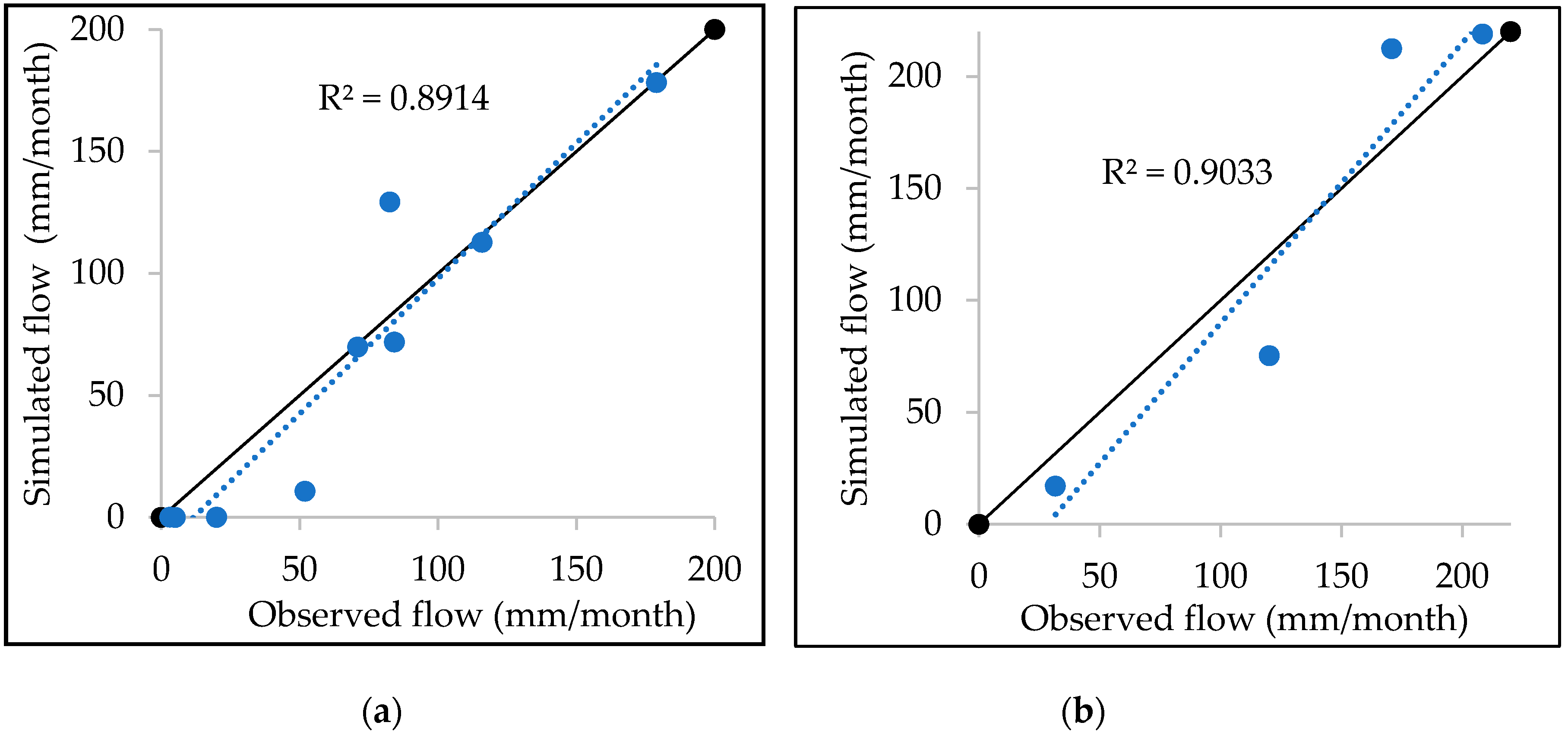
3.1. APEX Model Sensitivity Analysis, Calibration, and Validation for Hydrology and Crop Yield

All relevant parameters for APEX hydrology components were included in the sensitivity analysis based on Reference [40]. The results of the sensitivity analysis in the Dangishita watershed depicted that streamflow was sensitive to the following parameters: Hargreaves potential evapotranspiration (PET) equation exponent (PARM-34), runoff CN residue adjustment parameter (PARM-15), runoff volume adjustment factor (PARM-92), runoff CN initial abstraction (PARM-20), soil water lower limit (PARM-5), and soil evaporation coefficient (PARM-12), in order of decreasing influence (Table 4). The most sensitive parameters were associated with soil characteristics and climatic conditions. The parameter PARM-34 was found to be the most sensitive parameter for streamflow followed by PARM-15, possibly because ET was the second most-dominant hydrological process after rainfall. Reference [56] also found ET affecting the water yield of the catchment in their scenario analysis. Similarly, the sensitivity analysis results were found to be consistent with the findings of References [57]. Variable CN nonlinear CN/SW with depth soil water weighting method (NVCN = 0) was used, which is a function of soil water content and is directly linked with ET. Parameters PARM-92 and PARM-20 were found to be the third and fourth most sensitive parameters for streamflow prediction. Parameters APM and PARM-90 were less sensitive and thus not used for calibration.
The APEX hydrology model was calibrated using measured 1-year streamflow data (June 2015 to May 2016) (Figure 6a) followed by validation (June 2016 to October 2016) monthly (Figure 6b). Model parameter initialization was carried out prior to calibration (warm-up period: January 2010 to May 2015). Final calibrated values of sensitive parameters are listed in Table 4. The APEX model water yield simulation showed very good agreement with the observed monthly streamflow (both calibration and validation) based on statistical performance measure ratings proposed in Reference [58] for a monthly time step; NSE > 0.75 (very good), RSR ≤ 0.5 (very good), and PBIAS ≤ ±10% (very good). Also, the determination coefficient showed very good performance rating (R2 > 0.80) as based on Reference [59] for monthly streamflow comparison. The performance of the APEX hydrology model (monthly streamflow) for Dangishita watershed is shown in Table 5. The model slightly underestimated (Figure 6 and Figure 7) when the rainy season started to cease (October to January), perhaps due to the gauging station conditions (some stagnant water was observed at the gauging station and could affect the rating curve development for this specific period).

3.2. Dangishita and Robit Plot Level Model Parameters

Dangishita experimental plots were located within and in the proximity of the Dangishita watershed outlet. Calibrated watershed hydrology parameters (Table 4) were transferred to Dangishita experimental plots. No streamflow record was available for the Robit study site. The Dangishita and Robit sites have a similar agro-ecological zone [51] and have the same soil type (Chromic Luvisols), which are categorized under hydrologic soil group C. Similarly, calibrated parameters from the Dangishita watershed were transferred to the Robit site as well and used for hydrological analysis. Thus, the transferred parameters were used to evaluate the impacts of CA with drip irrigation on the hydrology of the system.

3.3. Yemu and Mkindo Plot Level Model Parameters

Parameters for Yemu were calibrated against simulated data for the nearby Tamale site [60]. Accordingly, values of some of the water balance components were obtained from the literature of the region or areas close to the study site (see Table 6). The plot level model was calibrated based on annual water balance components. Calibrated parameters (Table 7) were used to evaluate the impacts of CA with drip irrigation on hydrology for Yemu and Mkindo sites. APEX simulation for annual ET, Q, and PRK were in good agreement for both Yemu and Mkindo with the values from the literature for the Yemu and Mkindo sites. As per Reference [61], the performance rating is considered very good when PE is less than 15%. The Hargreaves PET method and daily CN nonlinear CN/SW with depth soil weighting were used and were found robust to simulate ET and Q, respectively, for the study sites.

3.4. Model Validation for Crop Yield

The APEX model was evaluated in predicting crop yield across the sites (Dangishita, Robit, Yemu, and Mkindo) for various vegetables (Table 2). The model successfully simulated vegetable yields for various climatic, soil, and environmental conditions under CA (with the “ADDMULCH” subroutine) and CT management. Overprediction occurred as often as under prediction for both CT and CA practices; however, model efficiency measures [45] were found to be very good for both calibration and validation across the study sites (Table 8).

3.5. Impact of CA on Hydrology and Water Management

The impacts of CA on hydrology were analyzed at a plot level for all sites (Table 9). A one-tailed paired t-test was conducted to examine the significance of CA in improving agricultural water management. Significant (α = 0.05) reductions were observed for water loss through ET, P(T <= t) = 0.007, and Q, P(T <= t) = 0.027, under CA across the sites for different cropping seasons and vegetables. ET was decreased in CA: 44–49%, 28–44%, 1–9%, and 1–11% for various vegetables and cropping seasons grown at Dangishita, Robit, Yemu, and Mkindo sites, respectively. Likewise, Q was reduced for CA: 17–54%, 34–62%, 2–12%, and 20% for different vegetables and cropping seasons at Dangishita, Robit, Yemu, and Mkindo sites, respectively. On the other hand, water saving was significantly (α = 0.05) increased under CA across the sites through increased PRK, P(T <= t) = 0.007, and RZSW, P(T <= t) = 0.0001, for various vegetables for different cropping seasons. PRK increased substantially under CA: 173–231%, 52–312%, 2–21%, and 25–91% in Dangishita, Robit, Yemu, and Mkindo sites, respectively. PRK in the study sites was mainly because of rainfall. Similarly, the average RZSW was increased under CA: 13–18%, 4–25%, 5–40%, and 7–21% for different vegetables at Dangishita, Robit, Yemu, and Mkindo sites, respectively. Farmers in Dangishita and Robit adopted different irrigation use for CA and CT plots based on their intrinsic knowledge of vegetable water need and moisture content of the soil. Meanwhile, farmers in Yemu and Mkindo applied an equal amount of irrigation water to both management system (the drip kits installed for the sites did not have separate switch control), and thus comparison was not made between CA and CT regarding irrigation use. Irrigation water use in Ethiopia (IRGA) was significantly (α = 0.05) reduced under CA, P (T <= t) = 0.0001, for various vegetables (14–35% reduction); however, the model result indicated that CA could not remove the need for irrigation in the region. The amount of rainfall (RF) during the growing period is shown in Table 9 (the rainfall in Dangishita and Robit sites was either at the beginning or at the end of the cropping period). The degree of CA impact varies depending on several factors including weather condition, water input, crop type, soil characteristics, and type and thickness of mulch.

4. Discussion

CA was found to significantly reduce water loss via evapotranspiration and surface runoff, and thus improved water saving through increased soil moisture and percolation. As a result, less irrigation needs were observed (14–35% reduced) for various vegetables under CA management (Table 9). As a result of soil disturbance (no till) and continuous soil cover using organic mulch, soil quality and soil structure must have been improved due to the fundamental principles of the CA practice. When an organic mulch material gets decomposed, it adds organic matter to the soil, which invites microorganisms (worms, bacteria, fungi, etc.). Microorganisms digest the organic matter and produce glue material that helps to stick small soil particles together and form aggregates; as such, soil pore space gets increased. Similarly, mulch cover avoids soil crusting, i.e., the breakdown and movement of small soil particles to the soil pore from the energy of dropping water, which creates a thin layer on the soil surface. Soil crusting greatly reduces infiltration. Thus, the soil structure, water holding capacity, and drainage was improved under CA resulting in higher water savings through higher percolation and soil moisture compared to CT (Table 9). The model considered the effects of mulch application on water management using “ADDMULCH” subroutine. This option changed the soil albedo and soil cover factor, which directly affected the computation of evapotranspiration, which further affected other hydrological variables. The no-till practice was captured in the model by providing zero-tillage depth in the tillage database of the model. Also, the rotation of vegetable production was integrated into the model through a management database.
CA reduced water loss through evaporation from the soil by providing shields from the sun and reducing soil heat, decreasing ET (Table 9). Reference [62] reported higher ET under CT in China when compared with conservation practice. The decrease in ET helps the soil to keep its moisture and consequently reduce irrigation water needs as seen in the Dangishita and Robit sites. Similarly, Reference [52] found increased infiltration and soil moisture under CA in Zimbabwe. Mulch application reduces water loss through reduction in runoff as it provides an obstacle on the soil surface and slows the movement of water, which provides extra time for the water to infiltrate into the soil [54,63,64]. In general, the degree of reduction in evapotranspiration and surface runoff varies depending on vegetable types, cropping seasons, water supply (precipitation and irrigation), weather conditions for the cropping periods, and other site-specific conditions. Furthermore, CA was found to increase water percolation significantly. Reference [65] reported a similar observation of significant increase in infiltration under CA in Australia.
The degree of improvements in agricultural water management was relatively less in Yemu and Mkindo when compared to the Dangishita and Robit sites. One reason could be due to the soil condition since the soil in Yemu is hydrologic group A, whereas the soil in Mkindo is hydrologic soil group D; the other two sites are hydrologic soil group C (Table 1). Hydrologic soil group A soils have good soil structure and drainage, which is evidenced by the low runoff and high percolation even under CT (Table 9). Hydrologic soil group D soils have poor soil structure and conditions, which are characterized by a very low infiltration rate and high runoff (Table 9). Therefore, the rate of improvement in soil structure for hydrologic soil groups A and D is expected to be relatively less since the soils were in very good and poor conditions, respectively, as compared to soil hydrologic group C. Another reason could be related to the vegetable types. For instance, farmers in Yemu grew sweet potato during the first cropping season in 2016, which has an extensive root system with higher water demand. Though soil evaporation was less under CA due to mulch cover, transpiration could have a significant contribution to ET due to sufficient water availability and the extensive root system of sweet potato. In addition, the amount of water input could be another reason for the relatively lower rate of water savings in Yemu and Mkindo. Reference [66] found a higher positive effect on CA with lower water input. Farmers in Dangishita and Robit applied less irrigation water to CA plots as compared to CT plots, whereas, farmers in Yemu and Mkindo applied the same amount of water for both CA and CT plots.

5. Conclusions

The impacts of CA on agricultural water management was analyzed through the integration of a field experiment and a biophysical model, APEX, at four study sites (Dangishita, Robit, Yemu, and Mkindo) in SSA. The APEX model was validated with a reasonable model performance using field-scale measurements (stream flow and crop yield) and the established literature. Once the APEX model was validated for hydrology and crop yield, the impacts of CA practices on water management was evaluated and compared with CT practice. Evapotranspiration, surface runoff, irrigation water, soil moisture in the root zone, and percolation below the root zone were compared between CA and CT systems under drip irrigation. Both evapotranspiration and surface runoff were found to decrease significantly (α = 0.05) under CA by up to 49% and 62%, respectively. Also, irrigation water use based on farmers’ practice was decreased significantly (α = 0.05) at the Dangishita and Robit sites for various seasons and vegetables (14–35%). In contrast, percolation and soil moisture were increased significantly (α = 0.05) under CA (up to 231% and 28%), respectively, as compared to CT. The increase in water savings was high for the Dangishita, Robit, and Mkindo sites compared to Yemu depending on soil conditions, selected vegetable types, and cropping periods. The results depicted significant improvement in soil structure and water-holding capacity across the sites. CA with drip irrigation was found to be a promising approach to improve water and soil management, and as a result, improve food production. It is essential and recommended to (1) provide thick mulch cover on the soil surface, and (2) introduce an irrigation scheduling approach based on actual evapotranspiration loss for the substantial improvement in soil quality and irrigation water management.

Author Contributions

T.A. contributed to the conceptual design, data collection and acquisition, data analysis and writing the manuscript. M.J. contributed to the conceptual design, data acquisition, data analysis, and revising the manuscript for the scientific content. M.R. contributed to the conceptual design, data acquisition, and analysis. A.W.W. contributed to the conceptual design, data acquisition, data analysis, and revising the manuscript for the scientific content.

Funding

This research and publication are made possible by the generous support of the American people through support by the United States Agency for International Development Feed the Future Innovation Labs for Collaborative Research on Small Scale Irrigation (Cooperative Agreement No. AID-OAA-A-13-0005, Texas A&M University) and Sustainable Intensification (Cooperative Agreement No. AID-OAA-L-14-00006, Kansas State University). The opinions expressed herein are those of the author(s) and do not necessarily reflect the views of the U.S. Agency for International Development.

Acknowledgments

We would like to acknowledge the National Meteorological Agency Services of Ethiopia, Amhara Design and Supervision Works Enterprise, and Ministry of Water and Energy of Ethiopia for providing us with quality data. The authors gratefully acknowledge the three anonymous reviewers for their valuable comments on our manuscript.

Conflicts of Interest

The authors declare no conflict of interest.

References

  1. Gebrehiwot, K.A.; Gebrewahid, M.G. The need for agricultural water management in sub-saharan Africa. J. Water Resour. Prot. 2016, 8, 835–843. [Google Scholar] [CrossRef]
  2. Bain, L.E.; Awah, P.K.; Geraldine, N.; Kindong, N.P.; Siga, Y.; Bernard, N.; Tanjeko, A.T. Malnutrition in Sub–Saharan Africa: Burden, causes and prospects. Pan Afr. Med. J. 2013, 15, 120. [Google Scholar] [CrossRef] [PubMed]
  3. Sheffield, J.; Wood, E.F.; Chaney, N.; Guan, K.; Sadri, S.; Yuan, X.; Olang, L.; Amani, A.; Ali, A.; Demuth, S. A drought monitoring and forecasting system for sub-Sahara African water resources and food security. Bull. Am. Meteorol. Soc. 2014, 95, 861–882. [Google Scholar] [CrossRef]
  4. Ozor, N.; Umunnakwe, P.C.; Acheampong, E. Challenges of food security in Africa and the way forward. Development 2013, 56, 404–411. [Google Scholar] [CrossRef]
  5. Devereux, S.; Maxwell, S. Food Security in Sub-Saharan Africa; ITDG Publishing: London, UK, 2001. [Google Scholar]
  6. Wiggins, S.; Keats, S. Leaping and Learning: Linking Smallholders to Markets in Africa; Agriculture for Impact, Imperial College and Overseas Development Institute: London, UK, 2013. [Google Scholar]
  7. Galhena, D.H.; Freed, R.; Maredia, K.M. Home gardens: A promising approach to enhance household food security and wellbeing. Agric. Food Secur. 2013, 2, 8. [Google Scholar] [CrossRef]
  8. Expósito, A.; Berbel, J. Sustainability implications of deficit irrigation in a mature water economy: A case study in southern Spain. Sustainability 2017, 9, 1144. [Google Scholar] [CrossRef]
  9. Busari, M.A.; Kukal, S.S.; Kaur, A.; Bhatt, R.; Dulazi, A.A. Conservation tillage impacts on soil, crop and the environment. Int. Soil Water Conserv. Res. 2015, 3, 119–129. [Google Scholar] [CrossRef] [Green Version]
  10. Palm, C.; Blanco-Canqui, H.; DeClerck, F.; Gatere, L.; Grace, P. Conservation agriculture and ecosystem services: An overview. Agric. Ecosyst. Environ. 2014, 187, 87–105. [Google Scholar] [CrossRef] [Green Version]
  11. González-Sánchez, E.; Ordóñez-Fernández, R.; Carbonell-Bojollo, R.; Veroz-González, O.; Gil-Ribes, J. Meta-analysis on atmospheric carbon capture in Spain through the use of conservation agriculture. Soil Tillage Res. 2012, 122, 52–60. [Google Scholar] [CrossRef]
  12. Le, K.N. Soil Organic Carbon Modeling with the EPIC Model for Conservation Agriculture and Conservation Tillage Practices in Cambodia. Ph.D. Thesis, North Carolina Agricultural and Technical State University, Greensboro, NC, USA, 2017. [Google Scholar]
  13. Hassanli, A.M.; Ahmadirad, S.; Beecham, S. Evaluation of the influence of irrigation methods and water quality on sugar beet yield and water use efficiency. Agric. Water Manag. 2010, 97, 357–362. [Google Scholar] [CrossRef]
  14. Howell, T.A. Irrigation efficiency. In Encyclopedia of Water Science; Marcel Dekke: New York, NY, USA, 2003; pp. 467–472. [Google Scholar]
  15. Jha, A.K.; Malla, R.; Sharma, M.; Panthi, J.; Lakhankar, T.; Krakauer, N.Y.; Pradhanang, S.M.; Dahal, P.; Shrestha, M.L. Impact of irrigation method on water use efficiency and productivity of fodder crops in Nepal. Climate 2016, 1, 13. [Google Scholar] [CrossRef]
  16. Postel, S.; Polak, P.; Gonzales, F.; Keller, J. Drip irrigation for small farmers: A new initiative to alleviate hunger and poverty. Water Int. 2001, 26, 3–13. [Google Scholar] [CrossRef]
  17. Expósito, A.; Berbel, J. Microeconomics of deficit irrigation and subjective water response function for intensive olive groves. Water 2016, 8, 254. [Google Scholar] [CrossRef]
  18. Marin, F.R.; Ribeiro, R.V.; Marchiori, P.E. How can crop modeling and plant physiology help to understand the plant responses to climate change? A case study with sugarcane. Theor. Exp. Plant Physiol. 2014, 26, 49–63. [Google Scholar] [CrossRef]
  19. Rauff, K.O.; Bello, R. A review of crop growth simulation models as tools for agricultural meteorology. Agric. Sci. 2015, 6, 1098–1105. [Google Scholar] [CrossRef]
  20. Hodson, D.; White, J. GIS and crop simulation modelling applications in climate change research. In Climate Change and Crop Production; CABI Publishers: Wallingford, UK, 2010; pp. 245–262. [Google Scholar]
  21. Adejuwon, J. Assessing the suitability of the EPIC crop model for use in the study of impacts of climate variability and climate change in West Africa. Singap. J. Trop. Geogr. 2005, 26, 44–60. [Google Scholar] [CrossRef]
  22. Ahmad, M.I.; Ali, A.; Ali, M.A.; Khan, S.R.; Hassan, S.W.; Javed, M.M. Use of crop growth models in agriculture: A review. Sci. Int. 2014, 26, 331–334. [Google Scholar]
  23. Wang, X.; Gassman, P.; Williams, J.; Potter, S.; Kemanian, A. Modeling the impacts of soil management practices on runoff, sediment yield, maize productivity, and soil organic carbon using APEX. Soil Tillage Res. 2008, 101, 78–88. [Google Scholar] [CrossRef]
  24. Antle, J.M.; Basso, B.; Conant, R.T.; Godfray, H.C.J.; Jones, J.W.; Herrero, M.; Howitt, R.E.; Keating, B.A.; Munoz-Carpena, R.; Rosenzweig, C. Towards a new generation of agricultural system data, models and knowledge products: Design and improvement. Agric. Syst. 2016, 155, 255–268. [Google Scholar] [CrossRef] [PubMed]
  25. Rivington, M.; Koo, J. Report on the Meta-Analysis of Crop Modelling for Climate Change and Food Security Survey; CGIAR Program on Climate Change, Agriculture and Food Security: Copenhagen, Denmark, 2010. [Google Scholar]
  26. Müller, C.; Elliott, J.; Chryssanthacopoulos, J.; Arneth, A.; Balkovic, J.; Ciais, P.; Deryng, D.; Folberth, C.; Glotter, M.; Hoek, S. Global gridded crop model evaluation: Benchmarking, skills, deficiencies and implications. Geosci. Model Dev. 2017, 10, 1403–1422. [Google Scholar] [CrossRef]
  27. Di Paola, A.; Valentini, R.; Santini, M. An overview of available crop growth and yield models for studies and assessments in agriculture. J. Sci. Food Agric. 2016, 96, 709–714. [Google Scholar] [CrossRef] [PubMed]
  28. Iizumi, T.; Yokozawa, M.; Sakurai, G.; Travasso, M.I.; Romanenkov, V.; Oettli, P.; Newby, T.; Ishigooka, Y.; Furuya, J. Historical changes in global yields: Major cereal and legume crops from 1982 to 2006. Glob. Ecol. Biogeogr. 2014, 23, 346–357. [Google Scholar] [CrossRef]
  29. Ray, D.K.; Ramankutty, N.; Mueller, N.D.; West, P.C.; Foley, J.A. Recent patterns of crop yield growth and stagnation. Nat. Commun. 2012, 3, 1293. [Google Scholar] [CrossRef] [PubMed] [Green Version]
  30. Moriasi, D.; Wilson, B.; Douglas-Mankin, K.; Arnold, J.; Gowda, P. Hydrologic and water quality models: Use, calibration, and validation. Trans. ASABE 2012, 55, 1241–1247. [Google Scholar] [CrossRef]
  31. Wang, X.; Kannan, N.; Santhi, C.; Potter, S.; Williams, J.; Arnold, J. Integrating APEX output for cultivated cropland with SWAT simulation for regional modeling. Trans. ASABE 2011, 54, 1281–1298. [Google Scholar] [CrossRef]
  32. Zhang, B.; Feng, G.; Read, J.J.; Kong, X.; Ouyang, Y.; Adeli, A.; Jenkins, J.N. Simulating soybean productivity under rainfed conditions for major soil types using APEX model in East Central Mississippi. Agric. Water Manag. 2016, 177, 379–391. [Google Scholar] [CrossRef]
  33. Gassman, P.W.; Williams, J.R.; Wang, X.; Saleh, A.; Osei, E.; Hauck, L.; Izaurralde, C.; Flowers, J. The Agricultural Policy Environmental Extender (APEX) model: An emerging tool for landscape and watershed environmental analyses. Trans. Am. Fish. Soc. Agric. Biol. Eng. 2010, 53, 711–740. [Google Scholar]
  34. Van Liew, M.W.; Wortmann, C.S.; Moriasi, D.N.; King, K.W.; Flanagan, D.C.; Veith, T.L.; McCarty, G.W.; Bosch, D.D.; Tomer, M.D. Evaluating the APEX Model for simulating streamflow and water quality on ten agricultural watersheds in the US. Trans. ASABE 2017, 60, 123–146. [Google Scholar]
  35. Tuppad, P.; Santhi, C.; Wang, X.; Williams, J.; Srinivasan, R.; Gowda, P. Simulation of conservation practices using the APEX model. Appl. Eng. Agric. 2010, 26, 779–794. [Google Scholar] [CrossRef]
  36. Clarke, N.; Bizimana, J.-C.; Dile, Y.; Worqlul, A.; Osorio, J.; Herbst, B.; Richardson, J.W.; Srinivasan, R.; Gerik, T.J.; Williams, J. Evaluation of new farming technologies in Ethiopia using the Integrated Decision Support System (IDSS). Agric. Water Manag. 2017, 180, 267–279. [Google Scholar] [CrossRef]
  37. Nachtergaele, F.; van Velthuizen, H.; Verelst, L.; Batjes, N.; Dijkshoorn, K.; van Engelen, V.; Fischer, G.; Jones, A.; Montanarella, L.; Petri, M. Harmonized World Soil Database; ISRIC: Wageningen, The Netherlands, 2009. [Google Scholar]
  38. Worqlul, A.W.; Ayana, E.K.; Maathuis, B.H.; MacAlister, C.; Philpot, W.D.; Leyton, J.M.O.; Steenhuis, T.S. Performance of bias corrected MPEG rainfall estimate for rainfall-runoff simulation in the upper Blue Nile Basin, Ethiopia. J. Hydrol. 2018, 556, 1182–1191. [Google Scholar] [CrossRef]
  39. Williams, J.R.; Arnold, J.G.; Srinivasan, R.; Ramanarayanan, T.S. APEX: A new tool for predicting the effects of climate and CO2 changes on erosion and water quality. In Modelling Soil Erosion by Water; Springer: New York, NY, USA, 1998; pp. 441–449. [Google Scholar]
  40. Wang, X.; Yen, H.; Liu, Q.; Liu, J. An auto-calibration tool for the Agricultural Policy Environmental eXtender (APEX) model. Trans. ASABE 2014, 57, 1087–1098. [Google Scholar]
  41. Francesconi, W.; Smith, D.R.; Heathman, G.C.; Wang, X.; Williams, C.O. Monitoring and APEX modeling of no-till and reduced-till in tile-drained agricultural landscapes for water quality. Trans. ASABE 2014, 57, 777–789. [Google Scholar]
  42. Saleh, A.; Gallego, O. Application of SWAT and APEX using the SWAPP (SWAT-APEX) program for the upper north Bosque River watershed in Texas. Trans. ASABE 2007, 50, 1177–1187. [Google Scholar] [CrossRef]
  43. Wang, X.; Hoffman, D.; Wolfe, J.; Williams, J.; Fox, W. Modeling the effectiveness of conservation practices at Shoal Creek watershed, Texas, using APEX. Trans. ASABE 2009, 52, 1181–1192. [Google Scholar] [CrossRef]
  44. Yin, L.; Wang, X.; Pan, J.; Gassman, P. Evaluation of APEX for daily runoff and sediment yield from three plots in the Middle Huaihe River Watershed, China. Trans. ASABE 2009, 52, 1833–1845. [Google Scholar] [CrossRef]
  45. Wang, X.; Williams, J.; Gassman, P.; Baffaut, C.; Izaurralde, R.; Jeong, J.; Kiniry, J. EPIC and APEX: Model use, calibration, and validation. Trans. ASABE 2012, 55, 1447–1462. [Google Scholar] [CrossRef]
  46. Williams, J.R.; Izaurralde, R.; Singh, V.; Frevert, D. The APEX model. In Watershed Models; Taylor & Francis: Boca Raton, FL, USA, 2006; pp. 437–482. [Google Scholar]
  47. NRCS, USDA. National Engineering Handbook: Part 630—Hydrology; USDA Soil Conservation Service: Washington, DC, USA, 2004.
  48. Green, W.H.; Ampt, G. Studies on Soil Phyics. J. Agric. Sci. 1911, 4, 1–24. [Google Scholar] [CrossRef]
  49. Williams, J.; Izaurralde, R.; Steglich, E. Agricultural Policy/Environmental Extender Model, Theoretical Documentation, Version 0806; 2008, Volume 604, pp. 2008–2017. Available online: https://agrilifecdn.tamu.edu/epicapex/files/2017/03/THE-APEX0806-theoretical-documentation-Oct-2015.pdf (accessed on 15 October 2018).
  50. Kumar, S.; Udawatta, R.P.; Anderson, S.H.; Mudgal, A. APEX model simulation of runoff and sediment losses for grazed pasture watersheds with agroforestry buffers. Agrofor. Syst. 2011, 83, 51–62. [Google Scholar] [CrossRef]
  51. Gebregiorgis, A.S.; Moges, S.A.; Awulachew, S.B. Basin regionalization for the purpose of water resource development in a limited data situation: Case of Blue Nile River Basin, Ethiopia. J. Hydrol. Eng. 2012, 18, 1349–1359. [Google Scholar] [CrossRef]
  52. Mupangwa, W.; Twomlow, S.; Walker, S. Reduced tillage, mulching and rotational effects on maize (Zea mays L.), cowpea (Vigna unguiculata (Walp) L.) and sorghum (Sorghum bicolor L.(Moench)) yields under semi-arid conditions. Field Crops Res. 2012, 132, 139–148. [Google Scholar] [CrossRef]
  53. Wang, X.; Harmel, R.; Williams, J.; Harman, W. Evaluation of EPIC for assessing crop yield, runoff, sediment and nutrient losses from watersheds with poultry litter fertilization. Trans. ASABE 2006, 49, 47–59. [Google Scholar] [CrossRef]
  54. Clausen, J.; Jokela, W.; Potter, F.; Williams, J. Paired watershed comparison of tillage effects on runoff, sediment, and pesticide losses. J. Environ. Qual. 1996, 25, 1000–1007. [Google Scholar] [CrossRef]
  55. Moriasi, D.N.; Arnold, J.G.; Van Liew, M.W.; Bingner, R.L.; Harmel, R.D.; Veith, T.L. Model evaluation guidelines for systematic quantification of accuracy in watershed simulations. Trans. ASABE 2007, 50, 885–900. [Google Scholar] [CrossRef]
  56. Feng, Q.; Chaubey, I.; Her, Y.G.; Cibin, R.; Engel, B.; Volenec, J.; Wang, X. Hydrologic and water quality impacts and biomass production potential on marginal land. Environ. Model. Softw. 2015, 72, 230–238. [Google Scholar] [CrossRef] [Green Version]
  57. Senaviratne, G. Apex and Fuzzy Model Assessment of Environmental Benefits of Agroforestry Buffers for Claypan Soils. Ph.D. Thesis, University of Missouri, Columbia, MO, USA, 2013. [Google Scholar]
  58. Moriasi, D.N.; King, K.W.; Bosch, D.D.; Bjorneberg, D.L.; Teet, S.; Guzman, J.A.; Williams, M.R. Framework to parameterize and validate APEX to support deployment of the nutrient tracking tool. Agric. Water Manag. 2016, 177, 146–164. [Google Scholar] [CrossRef]
  59. Vilaysane, B.; Takara, K.; Luo, P.; Akkharath, I.; Duan, W. Hydrological stream flow modelling for calibration and uncertainty analysis using SWAT model in the Xedone river basin, Lao PDR. Procedia Environ. Sci. 2015, 28, 380–390. [Google Scholar] [CrossRef]
  60. Anayah, F.M.; Kaluarachchi, J.J.; Pavelic, P.; Smakhtin, V. Predicting groundwater recharge in Ghana by estimating evapotranspiration. Water Int. 2013, 38, 408–432. [Google Scholar] [CrossRef]
  61. Bizimana, J.-C.; Clarke, N.P.; Dile, Y.T.; Gerik, T.J.; Jeong, J.; Leyton, J.M.O.; Richardson, J.W.; Srinivasan, R.; Worqlul, A.W. Ex Ante Analysis of Small-Scale Irrigation Interventions in Mvomero. ILSSI Reports and Publications. 2014. Available online: https://ilssi.tamu.edu/media/1295/small-scale-irrigation-applications-for-smallholder-farmers-in-tanzania.pdf (accessed on 15 September 2018).
  62. Su, Z.; Zhang, J.; Wu, W.; Cai, D.; Lv, J.; Jiang, G.; Huang, J.; Gao, J.; Hartmann, R.; Gabriels, D. Effects of conservation tillage practices on winter wheat water-use efficiency and crop yield on the Loess Plateau, China. Agric. Water Manag. 2007, 87, 307–314. [Google Scholar] [CrossRef]
  63. Fawcett, R. Agricultural tillage systems: Impacts on nutrient and pesticide runoff and leaching. In Farming for a Better Environment: A White Paper; Soil and Water Conservation Society: Ankeny, IA, USA, 1995; p. 67. [Google Scholar]
  64. Stagnari, F.; Ramazzotti, S.; Pisante, M. Conservation agriculture: A different approach for crop production through sustainable soil and water management: A review. In Organic Farming, Pest Control and Remediation of Soil Pollutants; Springer: New York, NY, USA, 2009; pp. 55–83. [Google Scholar]
  65. Bissett, M.J.; Oleary, G.J. Effects of conservation tillage and rotation on water infiltration in two soils in south-eastern Australia. Soil Res. 1996, 34, 299–308. [Google Scholar] [CrossRef]
  66. Qin, W.; Hu, C.; Oenema, O. Soil mulching significantly enhances yields and water and nitrogen use efficiencies of maize and wheat: A meta-analysis. Sci. Rep. 2015, 5, 16210. [Google Scholar] [CrossRef] [PubMed]
Figure 1. Location of experimental sites in SSA: (a) Yemu in Ghana, (b) Mkindo in Tanzania, and (c) Robit and (d) Dangishita in Ethiopia.
Sustainability 10 04763 g001
Figure 2. (a) Conservation agriculture (CA), and (b) conventional tillage (CT) plots, both under drip irrigation.
Sustainability 10 04763 g002
Figure 3. Location of Dangishita watershed and experimental plots.
Sustainability 10 04763 g003
Figure 4. Mean monthly rainfall for study sites (Dangishita, Robit, Yemu, and Mkindo).
Sustainability 10 04763 g004
Figure 5. APEX model major components (adapted from Wang, Yen, Liu and Liu [40]).
Sustainability 10 04763 g005
Figure 6. Comparison of measured and simulated stream flow for (a) calibration (June 2015–May 2016), and (b) validation (June–October 2016) periods for the Dangishita watershed.
Sustainability 10 04763 g006
Figure 7. Time series comparison of measured and simulated stream flow and corresponding precipitation data for the Dangishita watershed.
Sustainability 10 04763 g007
Table 1. Soil characteristics derived using SPAW hydrology [37].
Soil CharacteristicsChromic LuvisolsFerric LuvisolsFerallic Cambisols
Layer 1Layer 2Layer 1Layer 2Layer 1Layer 2
Texture classSandy clay loamSandy clay loamSandy loamSandy clay loamSandy clay loamClay loam
Wilting point (vol%)16.820.66.413.424.526.5
Field capacity (vol%)27.932.312.621.335.737.8
Soil water (cm/cm)0.110.120.060.080.130.11
Saturated hydraulic conductivity (mm/h)6.812.6855.113.731.710.51
Bulk density (g/cm3)1.541.521.561.611.471.49
% sand514579685148
% silt22211110108
% clay273410223944
Organic carbon (wt%)0.630.350.530.31.730.78
Organic matter (wt%)1.10.600.910.522.971.34
Hydrologic soil groupCAD
Table 2. Management activities and cropping pattern for the experimental sites.
SiteVegetableManagement ActivityDate
DangishitaGarlic (1st cycle)Tillage 1 10/13/2015 and 10/16/2015
Mulch application 210/25/2015
Planting10/28/2015
UREA application11/28/2015
Irrigation application11/6/2015–2/22/2016
Harvesting3/3/2016–3/4/2016
Onion (2nd cycle)Tillage 1 3/14/2016 and 3/16/2016
Mulch application 23/15/2016
Planting3/17/2016
Irrigation application3/15/2016–5/3/2016
Harvesting6/24/2016–6/26/2016
Garlic (3rd cycle)Tillage 1 2/15/2017
Mulch application 22/17/2017
Planting2/17/2017
DAP 3 application4/3/2017
Irrigation application2/17/2017–6/3/2017
Harvesting6/20/2017–6/22/2017
Tillage 1 9/2/2015
RobitTomato (1st cycle)Mulch application 210/23/2015
Planting10/24/2015
Malathion 4 application11/22/2015
Irrigation application10/24/2015–3/12/2016
Harvesting3/01/2017–3/15/2016
Garlic (2nd cycle)Tillage 1 3/19/2016
Mulch application 23/21/2016
Planting3/22/2016
Irrigation application3/23/2016–6/1/2016
Harvesting7/10/2016–7/18/2016
Cabbage (3rd cycle)Tillage 1 10/27/2016
Mulch application 211/8/2016
Planting11/9/2016
UREA 3 application12/20/2016, 12/28/2016, and 1/18/2017
Dimeto 40% 4 application11/15/2016, 11/25/2016, and 12/25/2016
Irrigation application11/9/2016–2/25/2017
Harvesting2/15/2017–2/26/2017
YemuSweet Potato (1st cycle)Tillage 1 8/8/2016
Mulch application 28/10/2016
Planting8/10/2016
DAP 3 application8/13/2016
UREA 3 application8/22/2016
Irrigation application8/23/2016–11/22/2017
Harvesting11/23/2016
Green Pepper and Cucumber (2nd cycle)Tillage 1 7/14/2017
Mulch application 27/14/2017
Planting7/14/2107
DAP 3 application-
UREA 3 application-
Irrigation application-
Harvesting11/1/2017
MkindoCabbage (1st cycle)Tillage 1 6/29/2016
Mulch application 27/1/2016
Planting7/1/2016
Irrigation application7/1/2016–9/2/2016
Harvesting9/3/2016
African Nightshade (2nd cycle)Tillage 1 7/6/2017
Mulch application 27/6/2017
Planting7/6/2017
Irrigation application7/6/2017–9/13/2017
Harvesting9/15/2017
Note: 1 Only for CT plots; 2 Only for CA plots; 3 Fertilizer; 4 Pesticide.
Table 3. Modified input parameters and methods in APEX files.
ParametersModified ValueMeaning
NVCN0Variable daily CN nonlinear CN/SW 1 with depth soil water weighting
ISW3Estimated using the Rawls method (dynamic)
IKAT0Turns off auto-potassium applications
IET4Hargreaves method
DRV4MUSLE 2 modified USLE 3
PARM60Cause no dormancy for winter-grown crops
PARM380Plant-soil water stress is strictly a function of soil water content
PARM861Increase in value increase upward movement
NIRR1The amount specified is applied
IRR5Drip irrigation
BIR0Manual irrigation
Note: 1 Soil water content, 2 Modified universal soil loss equation, 3 Universal soil loss equation.
Table 4. Sensitive parameters and final calibrated values for streamflow calibration.
Hydrology ParametersDescriptionParameter RangesRanking of InfluenceInitial ValueFinal Fitted Value
APMPeak runoff rate-rainfall energy adjustment factor0.1–1.0711.0
PARM (5)Soil water lower limit0.0–1.050.50.4
PARM (12)Soil evaporation coefficient1.5–2.562.51.512
PARM (15)Runoff CN residue adjustment parameter0.0–0.3200.25
PARM (20)Runoff CN initial abstraction0.05–0.440.20.191
PARM (34)Hargreaves PET equation exponent 0.5–0.610.5440.6
PARM (90)Subsurface flow factor1–100811
PARM (92)Runoff volume adjustment factor 0.1–2.0310.6
Table 5. APEX model performance on a monthly basis for the calibration and validation period at the Dangishita watershed.
Performance MeasuresCalibrationValidation
NSE0.850.77
RSR0.110.22
PBIAS (%)7.981.36
R20.890.90
Table 6. Calibrated water balance components for Yemu (2000–2005) and Mkindo (1980–2010).
Water Balance Variables[60], YemuCalibrated Model, YemuPE (%)[61], MkindoCalibrated Model, MkindoPE (%)
Mean annual ET6036040.2not used for Mkindo
Mean annual Q112108−3.6≈100109−9.0
Mean annual PRKnot used for Yemu≈290260−10.0
Table 7. Values of calibrated parameters for Mkindo and Yemu.
ParametersDescriptionInitial ValueFitted Value, YemuFitted Value, Mkindo
PARM (15)Runoff CN residue adjustment parameter0.00.0 a0.3 a
PARM (20)Runoff curve number initial abstraction0.20.180.24
PARM (23)Hargreaves PET equation coefficient0.00320.00310.0031
PARM (34)Hargreaves PET equation exponent0.500.5 a0.50 a
PARM (92)Runoff volume adjustment factor1.00.572.0
Note: a parameter not used for calibration.
Table 8. APEX model performance in predicting crop yield under CA and CT management.
Model PerformanceManagementNSEPBIASRSRR2
CalibrationCT0.97−10.40.060.99
CalibrationCA0.9311.80.090.99
ValidationCT0.96−11.00.060.98
ValidationCA0.958.90.060.99
Table 9. Impacts of CA on hydrology and water management.
SiteCropManagementET (mm)Q (mm)PRK (mm)IGRA (mm)RZSW (mm)
Dangishita Garlic
(RF = 203 mm)
CA23225254320114
CT4163086370102
% change for CA−44−17+195−13.5+12
Onion
(RF = 378 mm)
CA28030162140140
CT4206549215122
% change for CA−33−54+231−35+15
Garlic
(RF = 316 mm)
CA2528844295147
CT494186163130128
% change for CA−49−53+173+30.7+15
RobitTomato
(RF = 80 mm)
CA2485108280107
CT360137135096
% change for CA−31−61.5+52−20+12
Garlic
(RF = 641 mm)
CA229107381110137
CT409162186175115
% change for CA−44.0−34.0+10537.1+19
Cabbage
(RF = none)
CA251033305128
CT34908360100
% change for CA−28.1c+312−15.3+28
YemuSweet potato
(RF = 397 mm)
CA3734718114837
CT3774817714836
% change for CA−1.1−2.1+2.3b+3
Green pepper
(RF = 590 mm)
CA2183738857
CT2294232156
% change for CA−5−12+21d+2
Cucumber
(RF = 590 mm)
CA1584438860
CT1734837059
% change for CA−9.0−8+5.0d+2
MkindoCabbage
(RF = 19 mm)
CA1350511077
CT1520311077
% change for CA−11c+70b+c
African Nightshade
(RF = 167 mm)
CA30444221573
CT31052221572
% change for CA−2−20+91b+1.5
Cabbage
(RF = 12 mm)
CA18802.517575
CT19302.017574
% change for CA−3c+25b+1.5
Note: a—change expressed in number, b—no irrigation difference, c—no change, d—no irrigation.

