Monitoring NDVI Inter-Annual Behavior in Mountain Areas of Mainland Spain (2001–2016)


1
Departamento de Tecnología Química y Ambiental, Universidad Rey Juan Carlos, 28933 Móstoles, Spain
2
Departamento de Ciencias de la Educación, Universidad Rey Juan Carlos, 28032 Madrid, Spain
*
Author to whom correspondence should be addressed.
Sustainability 2018, 10(12), 4363; https://doi.org/10.3390/su10124363
Submission received: 20 September 2018
/
Revised: 18 November 2018
/
Accepted: 19 November 2018
/
Published: 23 November 2018
Abstract
:Currently, there exists growing evidence that warming is amplified with elevation resulting in rapid changes in temperature, humidity and water in mountainous areas. The latter might result in considerable damage to forest and agricultural land cover, affecting all the ecosystem services and the socio-economic development that these mountain areas provide. The Mediterranean mountains, moreover, which host a high diversity of natural species, are more vulnerable to global change than other European ecosystems. The protected areas of the mountain ranges of peninsular Spain could help preserve natural resources and landscapes, as well as promote scientific research and the sustainable development of local populations. The temporal statistical trends (2001–2016) of the MODIS13Q1 Normalized Difference Vegetation Index (NDVI) interannual dynamics are analyzed to explore whether the NDVI trends are found uniformly within the mountain ranges of mainland Spain (altitude > 1000 m), as well as in the protected or non-protected mountain areas. Second, to determine if there exists a statistical association between finding an NDVI trend and the specific mountain ranges, protected or unprotected areas are studied. Third, a possible association between cover types in pure pixels using CORINE (Co-ordination of Information on the Environment) land cover cartography is studied and land cover changes between 2000 and 2006 and between 2006 and 2012 are calculated for each mountainous area. Higher areas are observed to have more positive NDVI trends than negative in mountain areas located in mainland Spain during the 2001–2016 period. The growing of vegetation, therefore, was greater than its decrease in the study area. Moreover, differences in the size of the area between growth and depletion of vegetation patterns along the different mountains are found. Notably, more negatives than expected are found, and fewer positives are found than anticipated in the mountains, such as the Cordillera Cantábrica (C.Cant.) or Montes de Murcia y Alicante (M.M.A). Quite the reverse happened in Pirineos (Pir.) and Montes de Cádiz y Málaga (M.C.M.), among others. The statistical association between the trends found and the land cover types is also observed. The differences observed can be explained since the mountain ranges in this study are defined by climate, land cover, human usage and, to a small degree, by land cover changes, but further detailed research is needed to get in-depth detailed conclusions. Conversely, it is found that, in protected mountain areas, a lower NDVI pixels trend than expected (>20%) occurs, whereas it is less than anticipated in unprotected mountain areas. This could be caused by management and the land cover type.
1. Introduction
Mountains occupy 22% of the Earth’s surface and more than 900 million people live in them [1]. These zones also provide vital resources to a significant proportion of the global population [1], among which are food, fresh water, fuels, wood, medicinal plants, minerals, regulation of effects of natural hazards, tourism, and cultural heritage.
Mountains are one of the most vulnerable regions in the world. Recently, mountains worldwide have undergone dramatic changes [2]. Moreover, there exists growing evidence that a higher elevation means faster changes in temperature than at lower elevations [2]. It is crucial to find the correct management of mountain areas to oppose threats, such as the retreat of glaciers and decreases in the snowpack [3,4,5], changes in water ecosystems [6], changes in the hydrological cycle [7,8], and the rising shift of vegetation species distribution within changing global scenarios [9,10,11].
Mountains occupy slightly less than half of Spain’s total area. Most mountains are within the Mediterranean bioregion. European mountain and Mediterranean ecosystems are more vulnerable to global change than other European ecosystems [12] (increased risk of forest fires, erosion, and water availability, for example) causing the Mediterranean mountains, which are the main type in Spain, to suffer a loss of agricultural and forestry services. Some statistical models already have forecasted a migration of Mediterranean tree species to higher elevations and a related decline in temperate or cold-adapted tree populations during the 21st century [13]. Ruiz–Labourdette et al. [13] reported in their study how large areas in the world covered by cold-wet Euro–Siberian conifer and broad-leaved forest communities would be lost due to global warming. They also remarked how the major changes will occur for the Mediterranean species of conifers which are presently found at low mountain elevations.
Most countries and territories in the world have planned and declared protected zones to assure sustainable agriculture and preserve biodiversity [14]. These protected areas must be considered the paradigm of environmental sustainability [15].
Currently, protected areas cover nearly 28% of the Spanish terrestrial zones [16]. There are various protection policies to preserve natural assets, different landscapes and to provide sustainable development for the human populations that live in Spain. These protected areas have the most environmental policies of the 17 autonomous regions and the two autonomous cities in Spain [17]. There exist National Parks, which depend on Spanish government administration, Nature Reserves and Natural Parks regulated by regional law, Special Protection Areas and Sites of Community Importance, for example. Regional decrees control the latter under the European Directive [18]. Although substantial legislative effort has been made in Spain, it is necessary to further monitor and assess their protected areas [19].
The monitoring and analyzing of land cover and its ecological services in protected areas can be easily taken into account through remote sensing [20]. Land cover research, with the help of a satellite-derived normalized difference vegetation index (NDVI), brings valuable methodologies for biodiversity and conservation science that have been successfully proven for analyzing ecological responses to global change, assuring good nature management [21,22,23,24,25,26,27,28,29,30].
The NDVI is an estimation of the photosynthetically active radiation fraction which is absorbed by vegetation [31]. This vegetation index has been largely and successfully used to study global productivity over the past three decades [32,33,34,35]. The advent of moderate resolution imaging spectroradiometer (MODIS) NDVI 250 m data enabled studies of time series data to adapt higher-resolution applications. MODIS was launched in December 1999 and has been used frequently for time-series vegetation studies [34,36,37,38,39,40,41] due to its improved geometry, radiometry and quality, combined with its free charge policy distribution. MODIS data are captured by two sensors (Aqua and Terra satellites), and are distributed at various pre-processing levels. Additionally, concerning temporal distribution, MODIS images are available as both daily and composite products.
Under the framework of other NDVI studies conducted in Spanish mountainous areas in the past few decades, in which rising trends of this index [42,43,44,45,46] are reported to be related to global warming, the aims of the present work are:
- Analyzing if significantly temporal NDVI short-term trends (2001–2016) occurred in the mainland Spanish mountains.
- Studying if the possible patterns indicate a growing or decreasing trend for the different ranges due to their different climatic and vegetative conditions.
- Studying if there exists an association between NDVI significant trends and location in protected or unprotected mountain areas.
- Analyzing a possible association between NDVI trends and land cover types from mainland Spain.
- Calculating if land cover changes occurred between 2000–2006 and 2006–2012 in every mountain zone, which could explain the possible NDVI trends in every mountainous area.
2. Materials and Methods
2.1. Study Area
Table 1 shows the percentage of protected area within every mountain area studied, and the mountain name abbreviation. Figure 1 shows the map of the present paper’s study area. It must be noted that the lines in blue match the 1000 m elevation level and the black dotted lines indicate the total area of each mountain range.
The mountain relief in mainland Spain involves discontinuities and contrasts in climate. The most important factors in the definition of mountain climate are altitude, latitude, orientation, massif, and continental. Generally, for every 100 m increment in elevation, the temperature drops 0.5 °C [47,48,49], which means greater rainfall possibilities (including in the form of snow), increased frost and shrinkage of the vegetative period.
Mountain climate territories are those located more than 1000 m above sea level and, for that reason, only pixels with an altitude higher than 1000 m (see Figure 1) were the focus of this study. The mean annual temperature in those territories is lower than 10 °C, with mild summers (no month exceeds 22 °C) and cold winters (months with the average temperature below 0 °C). Additionally, there is abundant total annual precipitation (higher than 1000 mm) [47,48,49].
The study area can be divided into three major latitudinal regions: north peninsular mountains, continental mountains, and south peninsular mountains. Three floors or levels within these three major areas can be distinguished: subalpine forest floor (1000–1500 m), alpine forest floor (1500–2500 m) and snow forest floor (>2500 m).
North peninsular mountains receive a total annual precipitation greater than 1800 mm, where the subalpine floor forms a continuous band from M.L.G to the C.Cat. The typical vegetation here comprises conifers (Mediterranean zone) and deciduous forest (Atlantic zone). The average annual temperature is about 10 °C, and total annual precipitation exceeds 1100 mm. The maximum rainfall changes from winter (west) to autumn (east). The alpine forest floor (1500–2500 m) loses the continuity of the previous level and appears in isolated cores in the west and in the Pir., in which it reaches its maximum development. The temperatures are much more severe than those of the sub-alpine forest floor: annual averages are below 6 °C and, in these areas, the total precipitation usually is higher than 1200 mm. These general characteristics conceal pronounced anomalies, however, due to the orientation of the relief or to the different influences of the Atlantic and the Mediterranean. The shaded areas on the Mediterranean side keep the ground covered by snow for seven months, two more than in the sun, and the Atlantic influence doubles the rainfall (2500 mm) and better distributes it throughout the year, and raises average temperatures 2–4 °C. The vegetation of the alpine forest floor comprises conifers and deciduous forestland spaces and, in the highest altitude areas, meadows and shrubs.
The snow floor, above 2500 m, is reduced at the center of the Pir. The average annual temperatures are below 0 °C, the seasons are diluted before a winter that lasts more than ten months, and summer is a warm and short parenthesis. Precipitation reaches 3000 mm in some areas, where mosses or lichens can be found [47,48,49,50,51].
Continental mountains show total annual precipitation between 1000 and 1500 mm. Average yearly temperatures range between 6 and 10 °C. The winters (0 °C/−2 °C) are long and cold and the summers are warm (although always below 22 °C). The orientation of the continental mountain relief is zonal, which entails an outstanding dissymmetry between the north and south slopes. The former are cooler and cloudier than the latter, yet receives a higher volume of rainfall because the southwest winds are more humid than those from the northwest. Due to their altitude, interior reliefs are framed within the sub-alpine forest floor.
Finally, south peninsular mountains also show a subtropical mountain climate. The most outstanding characteristics which these zones present are lower winter temperatures than those of the previous climates mentioned. Summers are also warmer, although no month reaches 22 °C, which is widely exceeded in the surrounding lowlands. The average precipitation ranges between 800 and 1000 mm, but this amount oscillates significantly depending on the altitude and, especially, the proximity to the sea and exposure to the southwesterly winds. The maximum rainfall occurs in winter, followed by autumn and spring. The subtropical mountain suffers a deep drought in summer, like the rest of the territory of the peninsula to the southeast. Here, coniferous and deciduous forests and xerophytic plants are found [47,48,49,50,51].
Within these mountainous zones, we have also studied the protected zones, namely, the national parks and biogeographical regions in the continental zone and from mountains higher than 1000 m. Those protected areas represent a considerable percentage of the total mountainous area in mainland Spain and are a vast reservoir of natural richness.
2.2. CORINE (Co-Ordination of Information on the Environment) Land Cover Maps
The CORINE (Co-ordination of Information on the Environment) Land Cover (CLC) is a set of European environmental landscape maps [52]. These maps are a free download from the Land Copernicus project website. The vector version consists of a dataset at a scale of 1:100,000 and a minimum mapping unit of 25 ha [52].
The occupancy map of the CORINE Land Cover for 2006 (version 18.5) containing three levels of depth, which includes 44 types of land cover, is used in this study because it is from the middle of the period 2001–2016. The map of changes between 2000 and 2006 and between 2006 and 2012 is utilized to calculate percentages in the mountainous areas.
2.3. The NDVI from the Applied MODIS Dataset Used
The NDVI is a spectral index calculated from the reflectance in the red (R) and near-infrared (NIR) bands as follows [53]: NDVI = (NIR − R) / (NIR + R). The causal relationship between NDVI and the fraction of photosynthetically active radiation (FAPAR) or the net primary production of plants [54] has been demonstrated empirically for different systems [33,34,35]. The NDVI dataset of mountains within mainland Spain for the dates between 2001 and 2016 has been used.
The 16-day composite MODIS VI product from Terra (MOD13Q1), which shows a 250-m spatial resolution, is used. This dataset was downloaded from the Earth Data NASA website or the area of study (four tiles). The MODIS dataset was first processed by fusing the four tiles of every date between 2001 and 2016 (368 dates) with the help of an iterative process in TerrSet software [55]. Three hundred and sixty-eight images belonged to the 368 dates (one image every 16 days from 2001 to 2016, both inclusive).
The MOD13Q1 product provides a unique NDVI value (calculated with bands 1 and 2 of the MODIS sensor) every 16 days per pixel, allowing the composition of a gap-free temporal series. The MOD13Q1 provides a 16-day composite NDVI giving quality information from the layer of 250 m in terms of pixel reliability (PR), and acquisition dates from the 250 m 16 composite days of the year (CDOY) [56]. The PR layer informs about the pixels’ reliability. The CDOY layer provides the date each vegetation index value was acquired [56]. The MODIS team uses an algorithm which chooses the best available pixel value from all the acquisitions from the 16-day period. The criteria utilized to select the best pixel value is low clouds, low view angle and the highest NDVI [56]. The MOD13Q1 product provided NDVI values with an approximate frequency of 16 days and an indicator of reliability to assure goodness in the next procedure before use in the annual time-series process.
2.4. Smoothing Normalized Difference Vegetation Index (NDVI) Pixel Curves in Spain with TIMESAT Software (Filtering Noise NDVI Profiles)
Using the TIMESAT software, Jönsson and Eklundh [57] used data from all the pixels in the study area from each year to determine the shape of the final year’s curve.
TIMESAT provides processing methods based on least-squares fitting to the upper envelope of the vegetation indexes data (here the NDVI). An asymmetric Gaussian filtering method [57] was performed for calculating the NDVI from all pixels that made up the study area. The Gaussian method is an ordinary least-squares method, where data are fit to model functions. More detail about the functions that follow the TIMESAT software can be seen in Jönsson and Eklundh [57].
The PR information associated with every NDVI MODIS curve belonging to every pixel that comprised the study zone was considered. TIMESAT provides a weighting mechanism in which some values in the time series can be more influential than others, therefore, higher weights for high-quality retrievals and low weights for low-quality recoveries were assigned. Points assigned with lower weights in the smoothing procedure also have a minor influence on the curve fit [57].
Following getting the final smoothing curves of NDVI per pixel, the average of every pixel that comprises the study area (n = 368) per year (2001–2016) were calculated. Then, those pixels in which the NDVI value was less than zero were removed because they belonged to rocks and bare floor, not vegetation.
2.5. Temporal Trend Analyses
The average NDVI annual value per pixel from the smoothing NDVI pixel curves were calculated and described in Section 2.4 of the present paper, followed by the average NDVI annual pixel value which was evaluated in the serial correlation. The serial correlation defines how neighboring values in a series depend on each other. This serial correlation is usually used to detect trends in ecological time series [58].
A Theil–Sen estimator was used to examine the trends within each NDVI pixel smoothing curve (time-series) [59]. Theil–Sen’s slope is considered a potential replacement of ordinary least squares for linear regression that computes the median of the pair wise slopes of all data cases that meet the ranking criteria. Thus, Theil-Sen’s slope is not sensitive to outliers and is better than ordinary least squares for liner regression since it requires low a priori information of the measurement errors [60]. Next, the sign of the NDVI series trend was observed through the slope of the Theil–Sen regression performed. The positive-sign Theil–Sen slopes were those considered growing trends while the negative-sign Theil–Sen slopes were those considered browning (decreasing) trends of NDVI.
Subsequent to getting the Theil-Sen slopes from all the pixels of the study area, a Mann–Kendall test was used to detect the significance of the greening or browning trends [61,62]. The Mann–Kendall test is a robust non-parametric trend detection method. A significant trend was assumed when the z-statistic was less than 0.1 (90% confidence interval).
The Theil–Sen regression and the Mann–Kendall tests were performed using the Clark Labs TerrSet Earth Trends Modeler (ETM) [55]. ETM is an integrated suite of tools for the analysis of image time series data associated with Earth observation remote sensing images. Using these measures, one raster layer with the Mann–Kendall significance values and another raster layer with the Theil–Sen slopes from all the pixels of the study area were produced. Accompanying the last-mentioned dataset, with the help of a Geographic Information System (GIS) software, a layer in which the pixels with positive significant NDVI trends (growing NDVI trends (code = 1)), the pixels with negative NDVI trends (browning trends (code = −1)) and the pixels with non-significant trends (those with a Mann–Kendall z-statistic less than 0.1) (code = 0) was created. This layer, with the three classes (1, −1 and 0), was combined with the layer that contained the information of each mountain range (see Figure 1 and Table 1), as well as the layer with the protected or non-protected mountain zones and with the digital terrain model (DTM) from mainland Spain. Thus, pixels could be counted with significant positive (growing) and negative (browning) NDVI trends and without statistical trends per different mountains and per protected and non-protected areas. The chi-squared test of independence was used to determine if there was a significant relationship, first between the trend and the mountain categorical variables (Table 2 second row for more detail) and second, between the trend and the protection rather than the mountain categorical variable (Table 2 third row for more detail). The mountain variable had 13 categories which matched the 13 different mountains from the study area; protection had two groups that were the protected and non-protected zones in the mountains; and, the trend variable had three categories, positive (growing NDVI), negative (browning NDVI) and no significant trend of NDVI. chi-squared tests between the trend and protected variables per mountain range were applied (Table 2, fourth to final row for more detail).
The frequency of each group for one variable was compared across the types of the second nominal variable for every test performed. The data can be displayed in a contingency table where each row represents a category for one variable, and each column represents a group for the other variable.
Graphs of NDVI trend distribution along different altitudes by mountains were created to assess the possible relationship between the NDVI trend and the altitude.
The possible relationship between the variables trend (with positive, negative and non-trend categories) and the type of land cover also was studied. The CORINE Land Cover Map of 2006 (level 3) filtered to have only pure pixels of the categories (82% pureness) was used. Pixels of the CORINE Land Cover Map were almost pure or belonged to one category, making a buffer of 125 m (half the pixel size of MODIS data used) in the vector CORINE Land Cover Map. This method was used to get NDVI pixel purity belonging to at least 82% of the land cover. This form of having pure pixels was used by Arrogante-Funes et al. [63,64].
A chi-squared test between the trend and cover type in which the cover type was built up by the most representative land cover categories was conducted. Those categories were non-irrigated arable land (Non-Irri.), agro-forestry areas (Agro-For), broad-leaved forest (Broad-leav.), coniferous forest (Con. For), natural grasslands (Nat. Grass) and transitional woodland-shrub (Tran. Wood-shr.). The chi-squared test was performed in a general way (with the whole study area) and then, a chi-squared test with the same variables used in the general approach per each mountainous area was conducted. The chi-squared analyses included only those mountain-land cover combinations in which there were at least 30 pure pixels. For the chi-squared test we used R 3.5 version free software.
Finally, land cover changes by mountain with the CORINE Land Cover map of changes available from 2000–2006 and 2006–2012 were observed, and a Spearman rank correlation test between the areas with significant NDVI trends between 2001–2016 and the areas with land cover changes between 2000–2006 and 2006–2012, respectively, were performed.
3. Results
3.1. Temporal Normalized Difference Vegetation Index (NDVI) Trend along Different Altitudes
Figure 2 indicates how the distribution of the percentage of negative and positive significant trends from 2001–2016 at different altitudes in mainland Spain are different than the total of pixels that make up mainland Spain. The positive trend curve seems to be different than the negative one. It also is observable how the curve with the percentage of pixels that do not show trends is similar to the curve that represents the total of pixels that make up mainland Spain. Generally, these results suggest how the altitude might be related to having pixels with NDVI significant trends. Focusing on the elevation higher than 1000 m, the present article study area could show how the positive trends curve is similar to the total percentage curve and the non-trend curve, whereas, the negative one has percentages higher than those other curves already mentioned. This fact is presented overall between 1300–1900 m of altitude.
Figure 3 represents the percentage of pixels with negative or positive NDVI trends, non-trends and, finally, the total of pixels in each altitude higher than 1000 m, the mountainous zones within mainland Spain. Figure 3 shows how the curves from the negative and positive NDVI trends are different than the curve of distribution, which represents all the pixels in the mountainous systems. It shows at a glance how the 13 mountainous zones (Figure 3a–m) present differences in the trend distribution curves at different altitudes. It seems remarkable that, in general, the green line evolutions are more similar to the blue lines, than to the red lines. This implies that the greening (growth) in the vegetation patterns are near to the expected (pixels), whereas the red (decrease) in the vegetation trends are more different than expected.
3.2. Temporal Normalized Difference Vegetation Index (NDVI) Trend along Different Mountains and Protected Areas
Figure 4 shows how the positive NDVI trends of the pixels were more common than the negative patterns from 2001 to 2016. The percentage of pixels with significant negative trends were approximately 6.7%, whereas the portion of pixels with significant positive trends reached 11.4%.
The I.S. with 26% and the S.C with 15.5% mountainous zones were those that had the most area from the total without significant NDVI trends in the study area. The C.Cant., with 29.37%, was the mountainous range with the most pixels from the total with a significant NDVI negative trend in the study area. Finally, the mountain systems with the greatest number of pixels with a significant positive trend were the I.N., with 19.8%, and the Pir. ranges, with 19.6%. These patterns can be seen in Figure 2b.
Figure 2 demonstrates how there were mountains that had a predominance of significant NDVI negative trends, such as C.Cant. or L.G., whereas, it can be seen how I.N or M.V had a predominance of positive trends rather than negative ones. Another remarkable fact found in Figure 4 was that C.Cant., M.L.G. and I.S. mountains had most of the negative NDVI significant trends seem to match protected areas.
Figure 5 and Figure 6 are included to show the percentages of negative (red color bars) and positive (green color bars) trends, now calculated from the total area in each mountain (Figure 5) and within every mountain from the total protected area (Figure 6a), and the percentage of negative and positive trend pixels from the total non-protected area. The key results can be summarized as follows:
The mountainous system with the greatest percentage of significant NDVI trends from the total of each area was M.T.C.R. (more than 25% of all pixels of these mountains). By contrast, the mountainous systems with the lowest percentage of significant NDVI trend pixels were the I.S and the M.M.A.
It is also interesting to note that M.V, Pir., C.Cat., I.N and M.C.M. showed a great difference between the percentage of positive and negative pixels, with a predominance of positive ones (always the percentage of positive trend pixels higher than 19). In contrast, the greatest difference between negative and positive pixels within a mountainous system occurred in C.Cant. and M.T.C.R. (see Figure 5), with more positive pixels.
It seems remarkable how in C.Cant., M.L.G and, to a lesser extent, in M.T.C.R., M.M.A. and B.S. mountain ranges, there was a higher percentage of negative NDVI trends (2001–2016) in protected areas than in non-protected. A lower rate of positive NDVI trends was found in protected areas compared to non-protected ones. Regarding M.V., C.Cat. and M.C.M., the reverse was the case—a higher percentage of positive trends in protected than in non-protected zones and a lower percentage of negative ones in protected compared with non-protected areas (see Figure 6) was found.
The results from the chi-squared tests (see Table 2) showed how the categorical variables Significant trend (positive, negative and non-trend) and Mountain range statistically were associated. It also associated the Significant trend with the Protection trend (protected or non-protected) when the test was performed considering all the pixels that comprise the study area and, also, when the test was made separately by mountainous systems. Having significant trends, and even the sign of the NDVI trend (growing or decreasing in the NDVI value), is related to the mountain studied and to being within a protected or non-protected area in these mountain areas.
Figure 7 shows the graphs with the difference in percentage (X-axis) between the expected and the observed number of pixels with positive (growing), negative (decreasing) and no NDVI trend (equal). Figure 7a shows the differences by mountains and Figure 7b shows the differences calculated for the total mountainous area (>1000 m) including protected or not protected categories. Figure 8 shows the differences between expected and observed pixels with NDVI trends, but in every mountain-protected or mountain-not-protected zones.
Figure 7a shows how, from these mountainous systems that showed lesser observed pixels with NDVI positive trends in addition to higher observed pixels with NDVI negative trends, C.Cant., M.L.G. and M.T.C.R. were those in which the negative trends occurred more often than expected. Conversely, M.V., Pir, I.N., M.C.M., and C.Cat. showed fewer negative NDVI trends than expected, in addition to higher positive NDVI trends than expected by the statistics performed in the present paper (see also Figure 7a). Furthermore, in the cases of the last five mountain ranges mentioned, these differences between occurred and expected were higher than 45%.
Figure 7b shows how, in protected areas, the percentage of the difference between observed and expected NDVI negative trend pixels in protected areas were higher than 20%, while, in non-protected regions the reverse was the case. Alternatively, the positive NDVI trends were very similar between the observed and expected counts.
Figure 8a shows how, in the C.Cant. protected area, there were higher numbers of negative NDVI trend pixels than expected and fewer positive NDVI trend pixels than expected. The last-mentioned pattern occurred as a reverse case within the non-protected area of C.Cant. It happened in the same way for M.L.G; however, the percentage of the difference between expected and observed counts were lower than they were found within C.Cant. (See also Figure 8a,d). Figure 8i results reveal how the M.T.C.R in protected areas had a similar number of observed pixels to the NDVI trends to those expected; however, in the non-protected areas, M.T.C.R showed a higher negative NDVI trend of observed pixels than expected and also lower positive ones than expected.
Figure 8f,m showed how C.Cat. and M.C.M. had, in non-protected areas, more negative NDVI trend pixels than expected (difference between observed and expected counts higher than 50%) and, also, there was a lower percentage of positive than expected (difference between observed and expected counts higher than 40%). Regarding C.Cat., the difference between trend frequencies found and expected in the protected area were not high, nevertheless, in M.C.M. these differences were higher than in C.Cat. Considering the M.C.M. mountain range, the observed negative trends in the protected pixels were fewer than expected while, in contrast, the observed positive patterns were higher than expected.
3.3. Temporal Normalized Difference Vegetation Index (NDVI) Trends with Pure Pixels of Cover Types
The chi-squared results shown in Table 3 reveal how there also exists an association between the pure pixels with positive, negative or no trend and the land cover type. Table 4 shows the observed pixels by the most representative land covers in the study area. The most representative classes are the Con. For. and the Non-irri. followed by the Broad-leav. land cover type. The area of the total study area (3,084,612.94 ha in total) is observed with positive, negative and non-trend of NDVI by classes and the overall percentages of negative, positive and not trend are similar to those from the whole study area (as discussed in Section 3.2). The most common are the non-trend pixels, followed by the positive pixels which reached 10.16%, and then the negative trend pixels with a percentage of 7.34.
Figure 8 shows how Tran. Wood-shr. was the land cover type with the highest difference between observed and expected positive pixels (almost 80%). This difference revealed greater positive pixels than expected. Additionally, the number of negative pixels was lower than expected (difference smaller than 20%). Agro-for. and Non-Irri. were those with the highest difference between observed and expected NDVI negative trend pixels, with higher for anticipated than for observed. It also was found there were fewer positive than expected while Con. For., and the Broad-leav. were those cover types in which it was found the worst changes to the NDVI. Con. For. and the Broad-leav. showed greater negative NDVI trend pixels than expected. The NDVI evolution from 2001–2016 seems to be worse in Broad-leav. than in Con. For. because fewer positives were observed than expected while in Con. For greater positives were observed than expected (see Figure 9 for more detail).
3.4. Land Cover Change (2000–2006 and 2006–2012)
During the period between 2000 and 2006 changes in land cover in 0.89% of the total area were found, and from 2006 to 2012 changes in land cover were in 0.73% of the entire area (9,432,279.201 ha is the total area). Table 5 shows the percentage of change by mountains. It is observable how the mountains that had higher cover type changes were M.LG., I.S., S.C., and C.Cant. while the most changes were from forest categories to burnt areas and from regions burnt to shrub (these results are not shown in the text).
The results from the Spearman test of correlation performed between the area of change from 2000–2006, 2006–2012 and the areas with significant NDVI trends did not show significant (p-value > 0.05) correlation. Moreover, rho reached 0.2 and 0.3 respectively.
4. Discussion
This study analyzed short-term trends (growing and decreasing) of the NDVI over mountain areas (higher than 1000 m) in mainland Spain for the period from 2001 to 2016. The amount of space with growing (significant positive NDVI trends) and decreasing (significant negative NDVI trends) NDVI values were studied to see if differences were due to differences in the climatic, management and vegetation types of each mountain. Additionally, as the protection in mainland Spanish mountains is very important to preserve their vast biodiversity [16,65,66,67], the study of the NDVI evolution, differentiating between protected and not protected areas, was included. Finally, the behavior of the NDVI during these years was explored for differences between cover types using pure pixels (one land cover category) and to see if the land cover change during the period studied could explain the patterns in the NDVI behavior.
First of all, in mainland Spain the NDVI trends seem to show different patterns at different altitudes. These differences also appeared between mountain ranges. The differences in the trends observed within different altitudes in the study zone are not a new find because, in the Mediterranean mountains and, generally, in other parts of the world, the vegetation succession processes and, thus, the vegetation distribution, are dependent on spatial and topographic patterns such as altitude or slope and orientation. Iterations between topographic effects on hydrological processes are some of the factors most widely used in differentiating vegetation patterns [68,69,70,71,72,73] for that reason.
Generally, in the studied mountain ranges (elevation higher than 1000 m) a predominance of positive significant NDVI trends rather than negative ones (11.4% versus 6.7%) was found. These percentages were similar when pure pixels of the most representative land cover types in the study area were used (see Table 5 for more detail). These results are in line with the global greening trends observed in other remote sensing vegetation studies around the world, [33,35,74,75,76,77,78,79,80] and phenological field observations [81,82,83]. The studies cited provide evidence of an advance in the beginning of the growing season since three decades ago. The last study’s trends are related to the increase in the temperatures of spring–summer and, in general, to the increase in the mean annual temperatures in mainland Spain and, in general, around the world. An accumulation of growing degree days concentrated, overall in the eastern United States and Europe, also were reported.
Regarding the percentages of positive and negative significant NDVI trends studied, differences were found between mountain ranges in the study area that are explained by the human, climatic and topographic (altitude) variables. These differences in the trends found also were related to the type of land cover in the mountain, as results showed. Generally, Tran. and Wood-shr. were found to be the classes with growing trends of NDVI while, by contrast, Coniferous Forest and Broad-leaved forest were those that suffered a decline in the NDVI patterns. Non-Irrigated arable land and Agro-forestry areas were found to be the most stable. This stability might be caused by the human influence that exists, compared to the other land covers. Differences for the same land cover between mountains indicate that the NDVI short-trends found in this article are explained, in part, by land cover types and, in part, by climatic factors (growth in mean temperatures, for instance [46]).
Additionally, changes in cover types from 2000 to 2006 were found in 0.89% of the total area, while, from 2006 to 2012, changes in land cover were found in 0.72% of the area. These changes were, overall, due to fires that had caused a change from the transitional shrub or forest categories to burnt areas or regions burnt to transitional shrub land covers; however, the magnitude is much lower than the magnitude of the NDVI trend found. Additionally, a statistical correlation between the area with change and the area with NDVI trends by mountains was not seen, so the cover type changes possibly might explain the trends. Nonetheless, the land cover change definitively was not the principal cause of those NDVI significant trends. Thus, the patterns are explained by cover type, land cover changes (to a lesser extent) and by climatic factors. These explanations also are supported by other authors who reported how vegetation dynamics are driven by climate, in particular by precipitation, incoming radiation and temperature [84,85,86,87,88,89], nutrient availability, and short-term natural and anthropogenic disturbances (fires, logging, insect epidemics, land-use change, and agricultural management, for example) that can be crucial at various spatiotemporal scales [90,91,92,93].
Specifically, in the Mediterranean mountains of Spain, the vegetation trends during the past few decades have been related to the abandonment of traditional activities [43,51,94,95]. Vidal–Macua et al. [95] discuss how land use management and the disturbances that are caused by the activities in the different land covers have been and continue to be the main driving force in vegetation succession. Conversely, in the Iberian Peninsula, there has been a remarkable increase in temperatures and a decrease in precipitation over the past few decades [96,97,98], which has led to an increase in the severity of droughts, especially in the Mediterranean area [99,100,101,102]. Higher quantities of decreasing vegetation were found in the Atlantic area than in the Mediterranean area, which was an unexpected pattern.
Looking at the statistical results, it is observable how there exists a significant relationship between finding negative, positive NDVI trends or not finding trends, from 2001 to 2016, and the mountain zone study. Generally, the positive occurred more frequently than expected based on the mean and the negative less frequently than was expected (see Figure 7a). These results match with other findings reported in the literature that discuss how positive vegetation activity is recorded mainly in mountain areas within Mainland Spain [43,44,45,46,103]. Papagiannopoulou et al. [104] showed how, for the period from 1981 to 2010, the production of vegetation in mainland Spain was controlled in the north by temperature and incoming irradiation and in the center, south, and east mostly by the precipitation regime. Thus, mountain zones have precipitation as their limiting factor. Karneli et al. [105] and Khorchani et al. [46] showed that, when water is the limiting factor for vegetation growth, the land surface temperature–NDVI correlation is expected to be negative, however, when the limiting factor is the energy, the relationship between the two variables is anticipated to be positive. Mountain areas in Spain are characterized mainly by high precipitation values and positive climatic water balances. Although these areas are affected by drought periods, overall, in spring and summer the vegetation continues developing because water availability is still enough; thus, slightly more significant positive trends than expected were found as well as less negative trends than expected. Some studies discuss how even arid or semi-arid areas have seen an increase in the photosynthetic activity due to the increase of CO2 in the atmosphere as a result of human activities and the fertilization process [80,106].
It can be appreciated how, in mountain systems such as Montañas Vascas, Pirineos, Ibérico Norte, Cordillera Catalana, Sistema Central, and Béticas Sur and Montes de Cádiz y Málaga, a larger percentage of positive trends than expected was found and, in contrast, a smaller portion of negative trends than expected was found. These areas had seen increases in their photosynthetic activity during the time studied. These mountainous areas are within the Alpine and Mediterranean regions, so the increase in the temperature, joined with enough precipitation and tolerance to drought, resulted in more positive trends than expected. Mountains such as Cordillera Cantábrica, Montes de León y Galicia, Ibérico Sur, Montes de Toledo y Ciudad Real, Bética Sur o Montes de Murcia y Alicante had more pixels with negative trends and less with positive ones than expected. The photosynthetic activity began decreasing from 2001 to 2016 (see Figure 6a). The difference between the observable negative NDVI trends and the expected is notable, overall, in Cordillera Cantábrica, Montes de León y Galicia, Montes de Toledo y Ciudad Real y Montes de Murcia y Alicante.
Considering Cordillera Cantábrica, this pattern was observable mainly in the more Atlantic area, and the results are not expected because, in theory, the limiting factor was not the precipitation and the temperature has been slightly increasing in that area [46]. Currently, all research reported an increment in the NDVI value for the last three decades [42,79,107]. Khorchani et al. [46] showed how the correlation between NDVI and land surface temperature is not significant for most of the areas located in the northwest of Spain, so the temperature seems to not affect this pattern. The increase in the trees of the forest in the Cordillera Cantábrica (coniferous and broad-leaf forest) is controlled, in part, by the incoming energy and by the cloudy atmosphere. The climatic patterns in the northwest of Spain are controlled by the North Atlantic jet stream [108]. Recently, anomalies in the trajectory of the North Atlantic jet stream [109] were found that could be related to a decrease in the cloudy atmosphere or that could provoke more severe droughts in some critical months of the year for the growth of vegetation. Other authors have reported that Cordillera Cantábrica suffered a land degradation with high rates of land abandoned and fragmented, a severe overgrazing, and an increase in wildfire occurrence during the past few decades [110,111,112]. Other studies suggest that the Fagus sylvatica species in northern zones of Spain is less resistant to climatic change than those located in southern areas of Spain [113].
To conclude, all these factors explain finding more negative and less positive trends than expected in the northwest of Spain’s mountain area. It was interesting to further the research in these areas, and not just in the semi-arid or arid zones for which the number of climatic change studies to date is higher than for humid areas. The results in M.L.G could be explained along with the results in Cordillera Cantábrica. However, land degradation is not as high and the species are in a range in which they need less humidity than those in Cordillera Cantábrica [113], a fact that could explain the percentage of negative NDVI trend pixels being lower than those found in the Cordillera Cantábrica. M.T.C.R and M.M.A are limited by precipitation and droughts. The increase in temperature and the drought suffered in the past few decades in these two mountain ranges could result in a decrease in vegetation activity. Additionally, in Montes de Murcia y Alicante, the abandonment of crop areas and urban growth has been blamed until now [79,107,114] and could explain, in part, these patterns.
To assess the relationship between the NDVI trends and the protected or non-protected areas, the study’s statistical results show how there exists a significant association between the two variables. The negative NDVI trends occurred more frequently than expected in protected areas (with a difference between observed and expected higher than 20%) and, by contrast, less frequently than expected in non-protected areas (with a difference between observed and expected higher than 20%) (see Figure 7b for more information). These results match with those reported by Martinez–Fernández et al. [115], in which the authors observed a slight decline in natural surfaces in protected areas located in mainland Spain, with variations between the type of cover. They found that the transitional woodland shrub had a significant increase over 4% and, by contrast, more standing forest and open spaces with grasslands experienced a decline. This study’s mountain protected areas have a higher percentage of standing timber and grasslands than the transitional woodland shrub and, maybe for that reason, the negative trends occurred with a higher frequency than expected and, on the contrary, occurred in the protected areas which had more standing forest and grasslands. Climatic and management factors could cause the finding of less vegetation activity than expected in the protected mountain areas during the past few decades [115], however, to have a greater level of understanding of the causes, it is necessary to conduct more specific research.
Concerning the protection effectiveness, Rodriguez–Rodriguez [17] and Martinez–Fernandez [116] reported recent results in which they showed high levels of effectiveness in protected Spanish sites (National and Natural Parks and Natura network 2000) since the development of urban and more natural cover in those protected areas. Both explained how more resources are needed for proper management and to prevent the effects of global change in peninsular Spain overall, and specifically for the Natura network 2000, considering the latest global financial crisis could affect the development and management of these protected areas during the period studied here. It was found in Catalonia specific natural management programs that could, in part, explain why more positive trends than negative were found overall in the Cordillera Catalana protected area (for more details see Figure 6).
5. Conclusions
This study showed the NDVI trends in the mountain area (elevation >1000 m) within mainland Spain, one of the world’s most naturally biodiverse sites and also one of the most vulnerable to the effects of global change, using the MODIS 13Q1 dataset. There was a focus on protected and non-protected mountain areas because these areas can provide environmental sustainability in important mountain ranges. Additionally, the trends by cover type and the land cover changes that occurred from 2000 to 2006 and from 2006 to 2012 were analyzed to explain the trends found. The principal conclusions are summarized as follows.
Generally, a predominance of significant positive NDVI trends over negative ones was found, similar to the results reported for other European mountain systems, as well as Spain, during the last three decades. More positive and less negative trends than expected relative to the median were found. These results show how the trends observed were explained by land cover type and, to a small degree, by cover type changes (although the percentages of change are low). Different behaviors of the same land cover while located in different mountains indicated that climatic effects (temperature, and precipitation changes during the past few decades) and land cover changes reported in other studies caused the NDVI short-term trends in the current study area.
There were critical mountain ranges in which less positive or more negative than expected pixels were found. From past study results, Cordillera Cantábrica was expected to show a great majority of positive trends due to climatic conditions (increase of the land surface temperature and no higher episodes of annual precipitation accumulation). However, some aspects reported by other authors, such as anomalies in the North Atlantic jet stream, habitat fragmentations, land abandonment or the increase of the land surface temperature could lead to decreasing trends in vegetation that should be interesting for further study.
An association between NDVI trends in mountain protected areas or non-protected areas was found. Additionally, higher negative and less positive trends than expected were found in protected areas (with a difference higher than 20% between observed and expected). Less negative and higher positive than expected trend areas in non-protected sites (with a difference higher than 20% between observed and expected) were found. This general situation also occurred when each mountain was studied separately. The highest differences between observed and expected cases were recorded in Cordillera Cantábrica and Montes de Murcia y Alicante. These patterns could be due to the relationship with the land cover in these areas, and not mainly due to management issues. The present study characterizes the vegetation patterns occurring in the mainland Spanish mountains during the period 2001–2016 and their protected and not protected areas. It is necessary to further investigate, however, to understand and even predict what can happen in those essential reservoirs of service ecosystems in future years.
Author Contributions
P.A.-F. and C.J.N. conceived and designed the experiments; P.A.-F. and C.J.N. performed the experiments; P.A.-F., C.J.N., R.R.-C., analyzed the data, wrote parts, revised and improved the proposed article.
Funding
This research was funded by the Spanish Ministry of Economy, Industry and Competitiveness in the framework of the SOSTPARK project (CSO2014-54611-JIN).
Acknowledgments
The authors would like to thank the National Aeronautics and Space Administration for images and data provided. We also giving thanks to A.G. Bruzón and the anonymous reviewers for their comments and suggestions for improving the study.
Conflicts of Interest
The authors declare no conflict of interest.
References
- Grêt-Regamey, A.; Brunner, S.H.; Kienast, F. Mountain ecosystem services: Who cares? Mt. Res. Dev. 2012, 32, S23–S34. [Google Scholar] [CrossRef]
- Pepin, N.; Bradley, R.S.; Diaz, H.F.; Baraër, M.; Caceres, E.B.; Forsythe, N.; Fowler, H.; Greenwood, G.; Hashmi, M.Z.; Liu, X.D. Elevation-dependent warming in mountain regions of the world. Nat. Clim. Chang. 2015, 5, 424–430. [Google Scholar] [Green Version]
- Barry, R.G.; Chorley, R.J. Atmosphere, Weather and Climate; Routledge: London, UK, 2009. [Google Scholar]
- DeBeer, C.M.; Pomeroy, J.W. Modelling snow melt and snowcover depletion in a small alpine cirque, Canadian rocky mountains. Hydrol. Process. Int. J. 2009, 23, 2584–2599. [Google Scholar] [CrossRef]
- Dyurgerov, M.B. Mountain glaciers are at risk of extinction. In Global Change and Mountain Regions; Springer: Dordrecht, The Netherlands, 2005; pp. 177–184. [Google Scholar]
- Salerno, F.; Rogora, M.; Balestrini, R.; Lami, A.; Tartari, G.A.; Thakuri, S.; Godone, D.; Freppaz, M.; Tartari, G. Glacier melting increases the solute concentrations of Himalayan glacial lakes. Environ. Sci. Technol. 2016, 50, 9150–9160. [Google Scholar] [CrossRef] [PubMed]
- Foster, P. The potential negative impacts of global climate change on tropical montane cloud forests. Earth-Sci. Rev. 2001, 55, 73–106. [Google Scholar] [CrossRef]
- Tasser, E.; Leitinger, G.; Tappeiner, U. Climate change versus land-use change? What affects the mountain landscapes more? Land Use Policy 2013, 60, 60–72. [Google Scholar] [CrossRef]
- Grabherr, G. Alpine vegetation dynamics and climate change—A synthesis of long-term studies and observations. In Alpine Biodiversity in Europe; Springer: Berlin/Heidelberg, Germany, 2003; pp. 399–409. [Google Scholar]
- Körner, C. Mountain biodiversity, its causes and function. Ambio 2004, 13, 11–17. [Google Scholar]
- Gehrig-Fasel, J.; Guisan, A.; Zimmermann, N.E. Tree line shifts in the Swiss Alps: Climate change or land abandonment? J. Veg. Sci. 2007, 18, 571–582. [Google Scholar] [CrossRef]
- Schröter, D.; Cramer, W.; Leemans, R.; Prentice, C.I.; Araújo, M.B.; Arnell, N.W.; Bondeau, A.; Bugmann, H.; Carter, T.R.; Gracia, C.A. Ecosystem service supply and vulnerability to global change in Europe. Science 2005, 310, 1333–1337. [Google Scholar] [CrossRef] [PubMed]
- Ruiz-Labourdette, D.; Nogués-Bravo, D.; Ollero, H.S.; Schmitz, M.F.; Pineda, F.D. Forest composition in Mediterranean mountains is projected to shift along the entire elevational gradient under climate change. J. Biogeogr. 2012, 39, 162–176. [Google Scholar] [CrossRef]
- Dudley, N. Guidelines for Applying Protected Area Management Categories; International Union for Conservation of Nature (IUCN): Grand, Switzerland, 2008. [Google Scholar]
- Rodríguez-Rodríguez, D.; Martínez-Vega, J. Evaluación de la Eficacia de las Áreas Protegidas; Fundación BBVA: Bilbao, Spain, 2013. [Google Scholar]
- Múgica, M.; Martínez, C.; Atauri, J.A.; Gómez-Limón, J.; Puertas, J.; García, D. Anuario del estado de las áreas Protegidas en España; EUROPARC-España: Madrid, Spain, 2017; p. 135. [Google Scholar]
- Rodríguez-Rodríguez, D.; Martínez-Vega, J. Protected area effectiveness against land development in Spain. J. Environ. Manag. 2018, 215, 345–357. [Google Scholar] [CrossRef] [PubMed] [Green Version]
- Atauri, J.A.; De Lucio, J.V. The role of landscape structure in species richness distribution of birds, amphibians, reptiles and lepidopterans in Mediterranean landscapes. Landsc. Ecol. 2001, 16, 147–159. [Google Scholar] [CrossRef]
- Rodríguez-Rodríguez, D.; Martínez-Vega, J.; Tempesta, M.; Otero-Villanueva, M.M. Limited uptake of protected area evaluation systems among managers and decision-makers in Spain and the Mediterranean sea. Environ. Conserv. 2015, 42, 237–245. [Google Scholar] [CrossRef]
- Foley, J.A.; Asner, G.P.; Costa, M.H.; Coe, M.T.; DeFries, R.; Gibbs, H.K.; Howard, E.A.; Olson, S.; Patz, J.; Ramankutty, N. Amazonia revealed: Forest degradation and loss of ecosystem goods and services in the amazon basin. Front. Ecol. Environ. 2007, 5, 25–32. [Google Scholar] [CrossRef]
- Pettorelli, N.; Vik, J.O.; Mysterud, A.; Gaillard, J.-M.; Tucker, C.J.; Stenseth, N.C. Using the satellite-derived NDVI to assess ecological responses to environmental change. Trends Ecol. Evol. 2005, 20, 503–510. [Google Scholar] [CrossRef] [PubMed]
- Sannier, C.A.D.; Taylor, J.C.; Plessis, W.D. Real-time monitoring of vegetation biomass with NOAA-AVHRR in Etosha National Park, Namibia, for fire risk assessment. Int. J. Remote Sens. 2002, 23, 71–89. [Google Scholar] [CrossRef]
- Turner, D.P.; Ritts, W.D.; Cohen, W.B.; Gower, S.T.; Zhao, M.; Running, S.W.; Wofsy, S.C.; Urbanski, S.; Dunn, A.L.; Munger, J.W. Scaling gross primary production (GPP) over boreal and deciduous forest landscapes in support of MODIS GPP product validation. Remote Sens. Environ. 2003, 88, 256–270. [Google Scholar] [CrossRef]
- Mallegowda, P.; Rengaian, G.; Krishnan, J.; Niphadkar, M. Assessing habitat quality of forest-corridors through ndvi analysis in dry tropical forests of south India: Implications for conservation. Remote Sens. 2015, 7, 1619–1639. [Google Scholar] [CrossRef]
- Gillespie, T.W.; Ostermann-Kelm, S.; Dong, C.; Willis, K.S.; Okin, G.S.; MacDonald, G.M. Monitoring changes of NDVI in protected areas of southern California. Ecol. Indic. 2018, 88, 485–494. [Google Scholar] [CrossRef]
- Janssen, T.A.J.; Ametsitsi, G.K.D.; Collins, M.; Adu-Bredu, S.; Oliveras, I.; Mitchard, E.T.A.; Veenendaal, E.M. Extending the baseline of tropical dry forest loss in Ghana (1984–2015) reveals drivers of major deforestation inside a protected area. Boil. Conserv. 2018, 218, 163–172. [Google Scholar] [CrossRef]
- Pettorelli, N.; Chauvenet, A.L.M.; Duffy, J.P.; Cornforth, W.A.; Meillere, A.; Baillie, J.E.M. Tracking the effect of climate change on ecosystem functioning using protected areas: Africa as a case study. Ecol. Indic. 2015, 20, 269–276. [Google Scholar] [CrossRef]
- Nagendra, H.; Lucas, R.; Honrado, J.O.P.; Jongman, R.H.G.; Tarantino, C.; Adamo, M.; Mairota, P. Remote sensing for conservation monitoring: Assessing protected areas, habitat extent, habitat condition, species diversity, and threats. Ecol. Indic. 2013, 33, 45–59. [Google Scholar] [CrossRef]
- Peng, S.; Chen, A.; Xu, L.; Cao, C.; Fang, J.; Myneni, R.B.; Pinzon, J.E.; Tucker, C.J.; Piao, S. Recent change of vegetation growth trend in China. Environ. Res. Lett. 2011, 6, 044027. [Google Scholar] [CrossRef]
- Wen, Z.; Wu, S.; Chen, J.; Lü, M. NDVI indicated long-term interannual changes in vegetation activities and their responses to climatic and anthropogenic factors in the three gorges reservoir region, China. Sci. Total Environ. 2016, 574, 947–959. [Google Scholar] [CrossRef] [PubMed]
- Sellers, P.J. Canopy reflectance, photosynthesis and transpiration. Int. J. Remote Sens. 1985, 6, 1335–1372. [Google Scholar] [CrossRef] [Green Version]
- Running, S.W.; Nemani, R.R.; Heinsch, F.A.; Zhao, M.; Reeves, M.; Hashimoto, H. A continuous satellite-derived measure of global terrestrial primary production. BioScience 2004, 54, 547–560. [Google Scholar] [CrossRef]
- Myneni, R.B.; Keeling, C.D.; Tucker, C.J.; Asrar, G.; Nemani, R.R. Increased plant growth in the northern high latitudes from 1981 to 1991. Nature 1997, 386, 698–702. [Google Scholar] [CrossRef]
- Zhang, X.; Friedl, M.A.; Schaaf, C.B.; Strahler, A.H.; Hodges, J.C.F.; Gao, F.; Reed, B.C.; Huete, A. Monitoring vegetation phenology using MODIS. Remote Sens. Environ. 2003, 84, 471–475. [Google Scholar] [CrossRef]
- Stöckli, R.; Vidale, P.L. European plant phenology and climate as seen in a 20-year AVHRR land-surface parameter dataset. Int. J. Remote Sens. 2004, 25, 3303–3330. [Google Scholar] [CrossRef] [Green Version]
- Busetto, L.; Colombo, R.; Migliavacca, M.; Cremonese, E.; Meroni, M.; Galvagno, M.; Rossini, M.; Siniscalco, C.; Morra Di Cella, U.; Pari, E. Remote sensing of larch phenological cycle and analysis of relationships with climate in the alpine region. Glob. Chang. Boil. 2010, 16, 2504–2517. [Google Scholar] [CrossRef]
- Colombo, R.; Busetto, L.; Fava, F.; Di Mauro, B.; Migliavacca, M.; Cremonese, E.; Galvagno, M.; Rossini, M.; Meroni, M.; Cogliati, S. Phenological monitoring of grassland and larch in the Alps from TERRA and AQUA MODIS images. Rivista Italiana di Telerilevamento 2011, 43, 83–96. [Google Scholar]
- Hmimina, G.; Dufrêne, E.; Pontailler, J.Y.; Delpierre, N.; Aubinet, M.; Caquet, B.; De Grandcourt, A.; Burban, B.; Flechard, C.; Granier, A. Evaluation of the potential of MODIS satellite data to predict vegetation phenology in different biomes: An investigation using ground-based NDVI measurements. Remote Sens. Environ. 2013, 132, 145–158. [Google Scholar] [CrossRef]
- Eklundh, L.; Johansson, T.; Solberg, S. Mapping insect defoliation in scots pine with MODIS time-series data. Remote Sens. Environ. 2009, 113, 1566–1573. [Google Scholar] [CrossRef]
- Sesnie, S.E.; Dickson, B.G.; Rosenstock, S.S.; Rundall, J.M. A comparison of LANDSAT TM and MODIS vegetation indices for estimating forage phenology in desert bighorn sheep (Ovis canadensis nelsoni) habitat in the Sonoran desert, USA. Int. J. Remote Sens. 2012, 33, 276–286. [Google Scholar] [CrossRef]
- Song, Y.; Song, C.; Li, Y.; Hou, C.; Yang, G.; Zhu, X. Short-term effects of nitrogen addition and vegetation removal on soil chemical and biological properties in a freshwater marsh in Sanjiang Plain, Northeast China. Catena 2013, 104, 265–271. [Google Scholar] [CrossRef]
- Vicente-Serrano, S.M.; Heredia-Laclaustra, A. Nao influence on NDVI trends in the Iberian Peninsula (1982–2000). Int. J. Remote Sens. 2004, 25, 2871–2879. [Google Scholar] [CrossRef]
- Lasanta-Martínez, T.; Vicente-Serrano, S.M.; Cuadrat-Prats, J.M. Mountain Mediterranean landscape evolution caused by the abandonment of traditional primary activities: A study of the Spanish central Pyrenees. Appl. Geogr. 2005, 25, 47–65. [Google Scholar] [CrossRef]
- Hill, J.; Stellmes, M.; Udelhoven, T.; Röder, A.; Sommer, S. Mediterranean desertification and land degradation: Mapping related land use change syndromes based on satellite observations. Glob. Planet. Chang. 2008, 64, 146–157. [Google Scholar] [CrossRef]
- Del Barrio, G.; Harrison, P.A.; Berry, P.M.; Butt, N.; Sanjuan, M.E.; Pearson, R.G.; Dawson, T. Integrating multiple modelling approaches to predict the potential impacts of climate change on species’ distributions in contrasting regions: Comparison and implications for policy. Environ. Sci. Policy 2006, 9, 129–147. [Google Scholar] [CrossRef]
- Khorchani, M.; Vicente-Serrano, S.M.; Azorin-Molina, C.; García, M.; Martín-Hernández, N.; Peña-Gallardo, M.; El Kenawy, A.; Domínguez-Castro, F. Trends in LST over the peninsular Spain as derived from the AVHRR imagery data. Glob. Planet. Chang. 2018, 166, 75–93. [Google Scholar] [CrossRef]
- Rivas-Martínez, S.; Gandullo, J.M.; Serrada, R.; Allué, J.L.; Montero, J.L.; González, J.L. Mapa de Series de Vegetación de España y Memoria; del Ministerio de Agricultura, Pesca y Alimentación: Madrid, Spain, 1987.
- Rivas-Martínez, S. Mapa de Series, Geoseries y Geopermaseries de Vegetación de España; Asociación Española de Fitosociología: Sarriena, Spain, 2007. [Google Scholar]
- Aliaga, F.T. Geografía física de España0; National University of Distance Education: Madrid, Spain, 2003; p. 454. [Google Scholar]
- Recio, R.; Manuel, J. Biogeografía. Paisajes Vegetales y vida Animal, 1st ed.; Editorial Sintesis: Madrid, Spain, 1988. [Google Scholar]
- García-Ruiz, J.M. Geoecología de las Áreas de Montaña; Geoforma Ediciones: Madrid, Spain, 1990. [Google Scholar]
- European Environment Agency (EEA). CLC 2006 Technical Guidelines; European Environment Agency: Copenhagen, Denmark, 2007. [Google Scholar]
- Tucker, C.J.; Sellers, P.J. Satellite remote sensing of primary production. Int. J. Remote Sens. 1986, 7, 1395–1416. [Google Scholar] [CrossRef] [Green Version]
- Myneni, R.B.; Williams, D.L. On the relationship between FAPAR and NDVI. Remote Sens. Environ. 1994, 49, 200–211. [Google Scholar] [CrossRef]
- Eastman, J.R. Terrset; Clark University: Worcester, UK, 2015. [Google Scholar]
- Didan, K. MOD13Q1 MODIS/Terra Vegetation Indices 16-day L3 Global 250m SIN Grid V006. Available online: https://lpdaac.usgs.gov/dataset_discovery/modis/modis_products_table/mod13a1_v006 (accessed on 21 November 2018).
- Jönsson, P.; Eklundh, L. Seasonality extraction by function fitting to time-series of satellite sensor data. IEEE Trans. Geosci. Remote Sens. 2002, 40, 1824–1832. [Google Scholar] [CrossRef]
- Erasmi, S.; Schucknecht, A.; Barbosa, M.P.; Matschullat, J. Vegetation greenness in northeastern Brazil and its relation to Enso warm events. Remote Sens. 2014, 6, 3041–3058. [Google Scholar] [CrossRef] [Green Version]
- Sen, P.K. Estimates of the regression coefficient based on Kendall’s Tau. J. Am. Stat. Assoc. 1968, 63, 1379–1389. [Google Scholar] [CrossRef]
- Fernandes, R.; Leblanc, S.G. Parametric (modified Least Squares) and non-parametric (Theil-Sen) linear regressions for predicting biophysical parameters in the presence of measurement errors. Remote Sens. Environ. 2005, 95, 303–316. [Google Scholar] [CrossRef]
- Mann, H.B. Nonparametric tests against trend. Econ. J. Econ. Soc. 1945, 13, 245–259. [Google Scholar] [CrossRef]
- Kendall, M.G. Rank Correlation Methods, 4th ed.; Griffin: London, UK, 1970; p. 160. [Google Scholar]
- Arrogante-Funes, P.; Novillo, C.J.; Romero-Calcerrada, R.; Vázquez-Jiménez, R.; Ramos-Bernal, R.N. Relationship between MRPV model parameters from MISRL2 land surface product and land covers: A case study within Mainland Spain. ISPRS Int. J. Geo-Inf. 2017, 6, 353. [Google Scholar] [CrossRef]
- Arrogante-Funes, P.; Novillo, C.J.; Romero-Calcerrada, R.; Vázquez-Jiménez, R.; Ramos-Bernal, R.N. Evaluation of the consistency of the three MRPV model parameters provided by the MISR level 2 land surface products: A case study in Mainland Spain. Int. J. Remote Sens. 2018, 39, 3164–3185. [Google Scholar] [CrossRef]
- Mendoza-Fernández, A.; Pérez-García, F.J.; Medina-Cazorla, J.M.; Martínez-Hernández, F.; Garrido-Becerra, J.A.; Sánchez, E.S.; Mota, J.F. Gap analysis and selection of reserves for the threatened flora of eastern Andalusia, a hot spot in the eastern Mediterranean region. Acta Bot. Gallica 2010, 157, 749–767. [Google Scholar] [CrossRef]
- Cowling, R.M.; Rundel, P.W.; Lamont, B.B.; Kalin Arroyo, M.; Arianoutsou, M. Plant diversity in Mediterranean-climate regions. Trends Ecol. Evol. 1996, 11, 362–366. [Google Scholar] [CrossRef]
- Blanca, G.; Cueto, M.; Martínez-Lirola, M.J.; Molero-Mesa, J. Threatened vascular flora of Sierra Nevada (Southern Spain). Boil. Conserv. 1998, 85, 269–285. [Google Scholar] [CrossRef]
- Pons, X.; Solé-Sugrañes, L. A simple radiometric correction model to improve automatic mapping of vegetation from multispectral satellite data. Remote Sens. Environ. 1994, 48, 191–204. [Google Scholar] [CrossRef]
- Florinsky, I.V.; Kuryakova, G.A. Influence of topography on some vegetation cover properties. Catena 1996, 27, 123–141. [Google Scholar] [CrossRef]
- Allen, C.D.; Macalady, A.K.; Chenchouni, H.; Bachelet, D.; McDowell, N.; Vennetier, M.; Kitzberger, T.; Rigling, A.; Breshears, D.D.; Hogg, E.H.T. A global overview of drought and heat-induced tree mortality reveals emerging climate change risks for forests. For. Ecol. Manag. 2004, 259, 660–684. [Google Scholar] [CrossRef]
- Bennie, J.; Hill, M.O.; Baxter, R.; Huntley, B. Influence of slope and aspect on long-term vegetation change in British chalk grasslands. J. Ecol. 2006, 94, 355–368. [Google Scholar] [CrossRef] [Green Version]
- Serra, J.M.; Cristobal, J.; Ninyerola, M. A classification procedure for mapping topo-climatic conditions for strategic vegetation planning. Environ. Model. Assess. 2011, 16, 77–89. [Google Scholar] [CrossRef]
- Moeslund, J.E.; Arge, L.; Bøcher, P.K.; Dalgaard, T.; Ejrnæs, R.; Odgaard, M.V.; Svenning, J.-C. Topographically controlled soil moisture drives plant diversity patterns within grasslands. Biodivers. Conserv. 2013, 22, 2151–2166. [Google Scholar] [CrossRef]
- Zhou, L.; Tucker, C.J.; Kaufmann, R.K.; Slayback, D.; Shabanov, N.V.; Myneni, R.B. Variations in northern vegetation activity inferred from satellite data of vegetation index during 1981 to 1999. J. Geophys. Res. Atmos. 2001, 106, 20069–20083. [Google Scholar] [CrossRef] [Green Version]
- Bogaert, J.; Farina, A.; Ceulemans, R. Entropy increase of fragmented habitats: A sign of human impact? Ecol. Indic. 2005, 5, 207–212. [Google Scholar] [CrossRef]
- Slayback, D.A.; Pinzon, J.E.; Los, S.O.; Tucker, C.J. Northern hemisphere photosynthetic trends 1982–99. Glob. Chang. Boil. 2003, 9, 1–15. [Google Scholar] [CrossRef]
- Liu, Y.Y.; Van Dijk, A.I.J.M.; De Jeu, R.A.M.; Canadell, J.G.; McCabe, M.F.; Evans, J.P.; Wang, G. Recent reversal in loss of global terrestrial biomass. Nat. Clim. Chang. 2015, 5, 470–474. [Google Scholar] [CrossRef]
- Xu, C.; Liu, H.; Williams, A.P.; Yin, Y.; Wu, X. Trends toward an earlier peak of the growing season in northern hemisphere middle-latitudes. Glob. Chang. Boil. 2016, 22, 2852–2860. [Google Scholar] [CrossRef] [PubMed]
- Alcaraz-Segura, D.; Liras, E.; Tabik, S.; Paruelo, J.; Cabello, J. Evaluating the consistency of the 1982-1999 NDVI trends in the Iberian peninsula across four time-series derived from the AVHRR sensor: LTDR, GIMMS, FASIR, and PAL-II. Sensors 2009, 10, 1291–1314. [Google Scholar] [CrossRef] [PubMed]
- Fensholt, R.; Langanke, T.; Rasmussen, K.; Reenberg, A.; Prince, S.D.; Tucker, C.; Scholes, R.J.; Le, Q.B.; Bondeau, A.; Eastman, R. Greenness in semi-arid areas across the globe 1981–2007: An earth observing satellite based analysis of trends and drivers. Remote Sens. Environ. 2012, 121, 144–158. [Google Scholar] [CrossRef]
- Rutishauser, T.; Luterbacher, J.; Jeanneret, F.; Pfister, C.; Wanner, H. A phenology-based reconstruction of interannual changes in past spring seasons. J. Geophys. Res. Biogeosci. 2007, 112. [Google Scholar] [CrossRef] [Green Version]
- Studer, S.; Stökli, R.; Appenzeller, C.; Vidale, P.L. A comparative study of satellite and ground-based phenology. Int. J. Biometeorol. 2007, 51, 405–414. [Google Scholar] [CrossRef] [PubMed]
- Delbart, N.; Picard, G.; Le Toan, T.; Kergoat, L.; Quegan, S.; Woodward, I.A.N.; Dye, D.; Fedotova, V. Spring phenology in boreal Eurasia over a nearly century time scale. Glob. Chang. Boil. 2008, 14, 603–614. [Google Scholar] [CrossRef]
- Lucht, W.; Prentice, I.C.; Myneni, R.B.; Sitch, S.; Friedlingstein, P.; Cramer, W.; Bousquet, P.; Buermann, W.; Smith, B. Climatic control of the high-latitude vegetation greening trend and Pinatubo effect. Science 2002, 296, 1687–1689. [Google Scholar] [CrossRef] [PubMed]
- Nemani, R.R.; Keeling, C.D.; Hashimoto, H.; Jolly, W.M.; Piper, S.C.; Tucker, C.J.; Myneni, R.B.; Running, S.W. Climate-driven increases in global terrestrial net primary production from 1982 to 1999. Science 2003, 300, 1560–1563. [Google Scholar] [CrossRef] [PubMed]
- Piao, S.; Fang, J.; Zhou, L.; Zhu, B.; Tan, K.; Tao, S. Changes in vegetation net primary productivity from 1982 to 1999 in China. Glob. Biogeochem. Cy. 2005, 19. [Google Scholar] [CrossRef] [Green Version]
- Jiapaer, G.; Yi, Q.; Yao, F.; Zhang, P. Comparison of non-destructive LAI determination methods and optimization of sampling schemes in an open Populus euphratica ecosystem. Urban For. Urban Green. 2017, 26, 114–123. [Google Scholar] [CrossRef]
- Montaldo, N.; Albertson, J.D.; Mancini, M. Vegetation dynamics and soil water balance in a water-limited Mediterranean ecosystem on Sardinia, Italy. Hydrol. Earth Syst. Sci. Discuss. 2008, 5, 219–255. [Google Scholar] [CrossRef]
- Tagesson, T.; Fensholt, R.; Cropley, F.; Guiro, I.; Horion, S.; Ehammer, A.; Ardö, J. Dynamics in carbon exchange fluxes for a grazed semi-arid savanna ecosystem in West Africa. Agric. Ecosyst. Environ. 2015, 205, 15–24. [Google Scholar] [CrossRef]
- Fischer, E.; Riggs, L.; Leitner, P.; Villablanca, F.; Leeman, T.; McCarten, N.; Rogers, C. Development of a Population-Based Habitat Suitability Model for Salt Marsh Harvest Mouse to Guide Restoration Efforts in the North Bay Region. Available online: https://www.google.com.tw/url?sa=t&rct=j&q=&esrc=s&source=web&cd=1&ved=2ahUKEwjst4PgueTeAhULw7wKHcEHAYcQFjAAegQIARAC&url=https%3A%2F%2Fnrm.dfg.ca.gov%2FFileHandler.ashx%3FDocumentID%3D5548&usg=AOvVaw2bneSWCkOnORLb88eM1QRK (accessed on 21 November 2018).
- Reichstein, M.; Bahn, M.; Ciais, P.; Frank, D.; Mahecha, M.D.; Seneviratne, S.I.; Zscheischler, J.; Beer, C.; Buchmann, N.; Frank, D.C. Climate extremes and the carbon cycle. Nature 2013, 500, 287–295. [Google Scholar] [CrossRef] [PubMed]
- Le Quere, C. Budget, global carbon. Earth Syst. Sci. Data 2016, 8, 605–649. [Google Scholar] [CrossRef]
- Zhu, Q.; Zhong, Y.; Zhao, B.; Xia, G.-S.; Zhang, L. Bag-of-visual-words scene classifier with local and global features for high spatial resolution remote sensing imagery. IEEE Geosci. Remote Sens. Lett. 2016, 13, 747–751. [Google Scholar] [CrossRef]
- Jiménez-Olivenza, Y.; Rodríguez-Porcel, L.; Calvo-Caballero, L. Medio siglo en la evolución de los paisajes naturales y agrarios de Sierra Nevada. Boletín de la Asociación de Geógrafos Españoles 2015, 68, 205–232. [Google Scholar]
- Vidal-Macua, J.J.; Zabala, A.; Ninyerola, M.; Pons, X. Developing spatially and thematically detailed backdated maps for land cover studies. Int. J. Digit. Earth 2017, 10, 175–206. [Google Scholar] [CrossRef]
- López-Moreno, J.I.; Morán-Tejeda, E.; Vicente Serrano, S.M.; Lorenzo-Lacruz, J.; García-Ruiz, J.M. Impact of climate evolution and land use changes on water yield in the Ebro Basin. Hydrol. Earth Syst. Sci. 2011, 15, 311–322. [Google Scholar] [CrossRef] [Green Version]
- Del Río, S.; Cano-Ortiz, A.; Herrero, L.; Penas, A. Recent trends in mean maximum and minimum air temperatures over Spain (1961–2006). Theor. Appl. Clim. 2011, 109, 605–626. [Google Scholar] [CrossRef]
- El Kenawy, A.; López-Moreno, J.I.; Vicente-Serrano, S.M. Trend and variability of surface air temperature in northeastern Spain (1920–2006): Linkage to atmospheric circulation. Atmos. Res. 2012, 106, 159–180. [Google Scholar] [CrossRef]
- Bernstein, L.; Bosch, P.; Canziani, O.; Chen, Z.; Christ, R.; Riahi, K. IPCC, 2007: Climate Change 2007: Synthesis Report; Intergovernmental Panel on Climate Change (IPCC): Geneva, Switzerland, 2008. [Google Scholar]
- Stocker, T.F.; Qin, D.; Plattner, G.K.; Tignor, M.; Allen, S.K.; Boschung, J.; Nauels, A.; Xia, Y.; Bex, V.; Midgley, P.M. IPCC, 2013: Climate Change 2013: The Physical Science Basis; Cambridge University Press: Cambridge, UK; New York, NY, USA, 2013; p. 1535. [Google Scholar]
- Gonzalez-Hidalgo, J.C.; López-Bustins, J.A.; Štepánek, P.; Martin-Vide, J.; de Luis, M. Monthly precipitation trends on the Mediterranean fringe of the Iberian Peninsula during the second-half of the twentieth century (1951–2000). Int. J. Clim. 2009, 29, 1415–1429. [Google Scholar] [CrossRef]
- Vicente-Serrano, S.M.; Lopez-Moreno, J.I.; Beguería, S.; Lorenzo-Lacruz, J.; Sanchez-Lorenzo, A.; Garcí-Ruiz, J.M.; Azorin-Molina, C.; Morán-Tejeda, E.; Revuelto, J.; Trigo, R. Evidence of increasing drought severity caused by temperature rise in southern Europe. Environ. Res. Lett. 2014, 9, 044001. [Google Scholar] [CrossRef] [Green Version]
- Vicente-Serrano, S.M.; Lasanta, T.; Romo, A. Analysis of spatial and temporal evolution of vegetation cover in the Spanish central Pyrenees: Role of human management. Environ. Manag. 2004, 34, 802–818. [Google Scholar] [CrossRef] [PubMed]
- Papagiannopoulou, C.; Miralles, D.G.; Dorigo, W.A.; Verhoest, N.E.C.; Depoorter, M.; Waegeman, W. Vegetation anomalies caused by antecedent precipitation in most of the world. Environ. Res. Lett. 2017, 12, 074016. [Google Scholar] [CrossRef] [Green Version]
- Karnieli, A.; Agam, N.; Pinker, R.T.; Anderson, M.; Imhoff, M.L.; Gutman, G.G.; Panov, N.; Goldberg, A. Use of NDVI and land surface temperature for drought assessment: Merits and limitations. J. Clim. 2010, 23, 618–633. [Google Scholar] [CrossRef]
- Canadell, J.G.; Le Quéré, C.; Raupach, M.R.; Field, C.B.; Buitenhuis, E.T.; Ciais, P.; Conway, T.J.; Gillett, N.P.; Houghton, R.A.; Marland, G. Contributions to accelerating atmospheric CO2 growth from economic activity, carbon intensity, and efficiency of natural sinks. Proc. Natl. Acad. Sci. USA 2007, 104, 18866–18870. [Google Scholar] [CrossRef] [PubMed] [Green Version]
- Martínez, B.; Gilabert, M.A. Vegetation dynamics from NDVI time series analysis using the wavelet transform. Remote Sens. Environ. 2009, 113, 1823–1842. [Google Scholar] [CrossRef]
- Vicente-Serrano, S.M.; Cuadrat, J.M. North Atlantic oscillation control of droughts in north-east Spain: Evaluation since 1600 ad. Clim. Chang. 2007, 85, 357–379. [Google Scholar] [CrossRef]
- Trouet, V.; Babst, F.; Meko, M. Recent enhanced high-summer north Atlantic Jet variability emerges from three-century context. Nat. Commun. 2018, 9, 180. [Google Scholar] [CrossRef] [PubMed]
- García-Ruiz, J.M.; Lana-Renault, N. Hydrological and erosive consequences of farmland abandonment in Europe, with special reference to the Mediterranean regional review. Agric. Ecosyst. Environ. 2011, 140, 317–338. [Google Scholar] [CrossRef]
- Blanco-Fontao, B.; Quevedo, M.; Obeso, J.R. Abandonment of traditional uses in mountain areas: Typological thinking versus hard data in the Cantabrian Mountains (NW Spain). Biodivers. Conserv. 2011, 20, 1133–1140. [Google Scholar] [CrossRef]
- Rodrigues, M.; Jiménez-Ruano, A.; Peña-Angulo, D.; de la Riva, J. A comprehensive spatial-temporal analysis of driving factors of human-caused wildfires in Spain using geographically weighted logistic regression. J. Environ. Manag. 2018, 225, 177–192. [Google Scholar] [CrossRef] [PubMed]
- Herrero, A.; Zavala, M.A. Los bosques y la Biodiversidad Frente al Cambio Climático: Impactos, Vulnerabilidad y Adaptación en España; Ministerio de Agricultura, Alimentación y Medio Ambiente: Madrid, Spain, 2015.
- Udelhoven, T.; Stellmes, M. Changes in land surface conditions on the Iberian Peninsula (1989 to 2004) detected by means of time series analysis from hypertemporal remote sensing data. In Proceedings of the 2007 International Workshop on the Analysis of Multi-Temporal Remote Sensing Images (MultiTemp 2007), Leuven, Belgium, 18–20 July 2007; pp. 1–6. [Google Scholar]
- Martinez-Fernandez, J.; Ruiz-Benito, P.; Zavala, M.A. Recent land cover changes in Spain across biogeographical regions and protection levels: Implications for conservation policies. Land Use Pol. 2015, 44, 62–75. [Google Scholar] [CrossRef]
- Martinez-Fernandez, J.; Ceballos, A. Mean soil moisture estimation using temporal stability analysis. J. Hydrol. 2005, 312, 28–38. [Google Scholar] [CrossRef]
Figure 1.
Mountain ranges in mainland Spain. Near each mountain range is the abbreviation name of the mountain. The lines in blue within each range refer to the level curve of 1000 m of height. Abbreviations are reported in Table 1.
Figure 1.
Mountain ranges in mainland Spain. Near each mountain range is the abbreviation name of the mountain. The lines in blue within each range refer to the level curve of 1000 m of height. Abbreviations are reported in Table 1.

Figure 2.
Relative percentage of pixels (Y-axis) with a significant NDVI trend along altitude in meters (X-axis) in the whole of mainland Spain. It must be noted that the percentage shown on the Y-axis refers to the total number of pixels belonging to all mainland Spain with a negative NDVI trend (red), the non-NDVI trend (yellow), positive NDVI trend (green) and the total pixels (blue).

Figure 3.
Percentage of pixels (Y-axis) with significant NDVI trends along different altitudes, expressed in meters, (X-axis) higher than 1000 meters for Mountain ranges in Mainland Spain. (a) Cordillera Cantábrica. (b) Montañas Vascas. (c) Pirineos. (d) Montes de León y Galicia. (e) Sistema Ibérico Norte. (f) Cordilleras Catalanas. (g) Sistema Central. (h) Sistema Ibérico Sur. (i) Montes de Toledo y Ciudad Real. (j) Montañas Béticas Norte. (k) Montes de Murcia y Alicante (l) Montañas Béticas Sur. (m) Montes de Cádiz y Málaga.

Figure 4.
(a) Study area. The protected areas are national parks and biogeographical regions of the continental zone from mountains in Spain higher than 1000 m. (b) Pixels with NDVI trends (p-value < 0.1) during the 2001–2016 period.
Figure 4.
(a) Study area. The protected areas are national parks and biogeographical regions of the continental zone from mountains in Spain higher than 1000 m. (b) Pixels with NDVI trends (p-value < 0.1) during the 2001–2016 period.

Figure 5.
Percentage of pixels (Y-axis) with significant NDVI positive (green) and negative (red) trends from the total pixels that make up every mountain range (X-axis). Contained in every positive and negative bar is the exact percentage of the NDVI trend from the total pixels in every protected and non-protected mountainous system. Abbreviations are reported in Table 1.

Figure 6.
Percentage of pixels (Y-axis) with significant NDVI positive (green) and negative (red) trends from the total pixels that make up every mountain range (X-axis). (a) The percentage is calculated from the total of pixels which built up the protected areas in every mountain. (b) The percentage is calculated from the total of pixels which built up the non-protected areas in every mountain. Contained in every positive and negative bar is the exact percentage of NDVI trends from the total pixels in each protected and non-protected mountainous system. Abbreviations are reported in Table 1.

Figure 7.
Difference in percentage between observed and expected pixels with positive (green), negative (red) and non-trend (grey) calculated considering mountains (a), and by protected and non-protected areas (b). Abbreviations are reported in Table 1.
Figure 7.
Difference in percentage between observed and expected pixels with positive (green), negative (red) and non-trend (grey) calculated considering mountains (a), and by protected and non-protected areas (b). Abbreviations are reported in Table 1.

Figure 8.
Difference in percentage between observed and expected pixels with positive (green), negative (red) and non-trend (grey). (a) Cordillera Cantábrica (C.Cant.). (b) Montañas Vascas (M.V.). (c) Pirineos (Pir.). (d) Montes de León y Galicia (M.L.G.). (e) Ibérico Norte (I.N.). (f) Cordilleras Catalanas (C.Cat.). (g) Sistema Central (S.C.). (h) Ibérico Sur (I.S.). (i) Montes de Toledo y Ciudad Real (M.T.C.R.). (j) Béticas Norte (B.N.). (k) Montes de Murcia y Alicante (M.M.A.) (l) Montañas Béticas Sur (B.S.). (m) Montes de Cádiz y Málaga (M.C.M.).

Figure 9.
Difference in percentage between observed and expected pixels with positive (green), negative (red) and with non-trend (grey).
Figure 9.
Difference in percentage between observed and expected pixels with positive (green), negative (red) and with non-trend (grey).


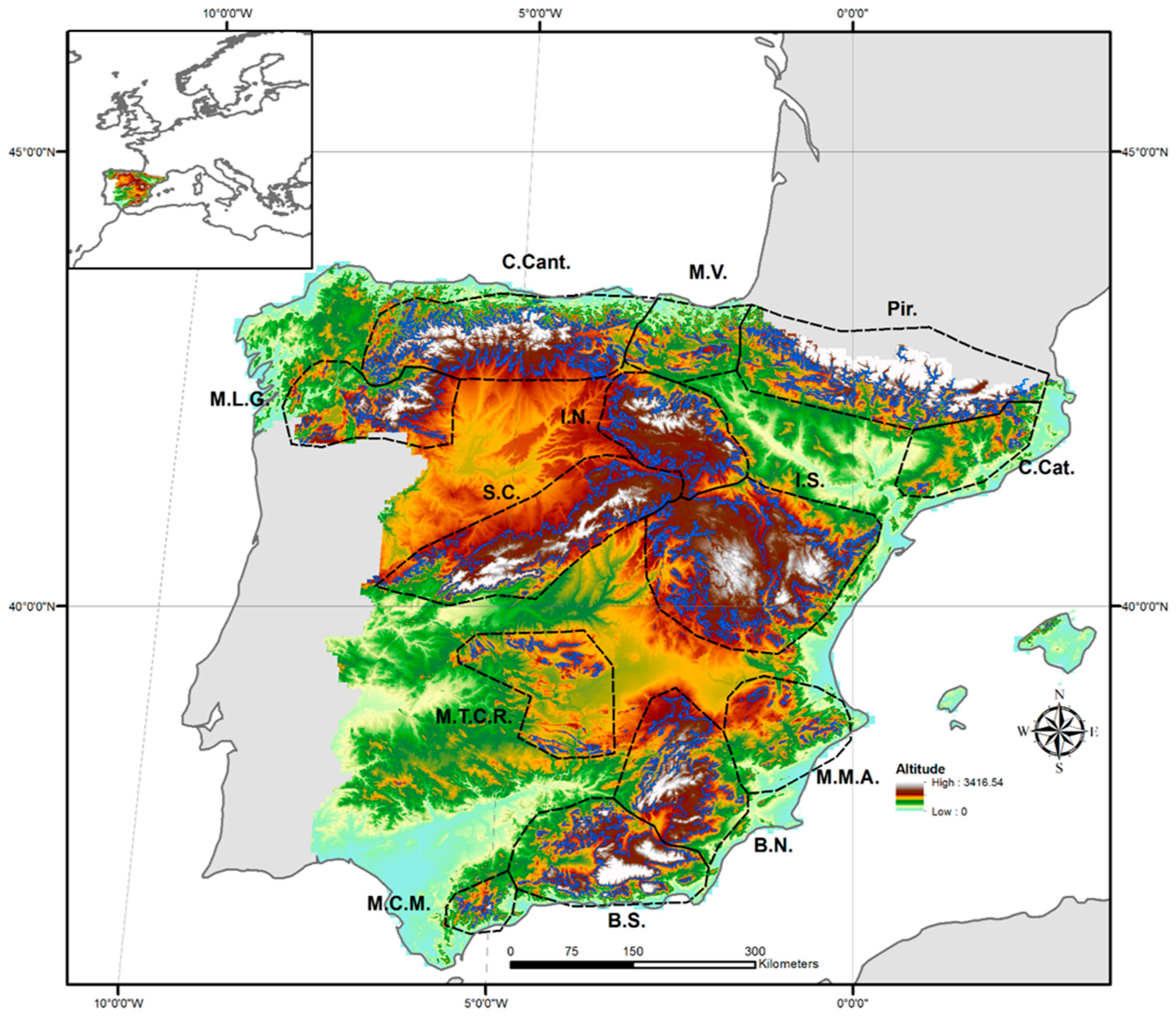
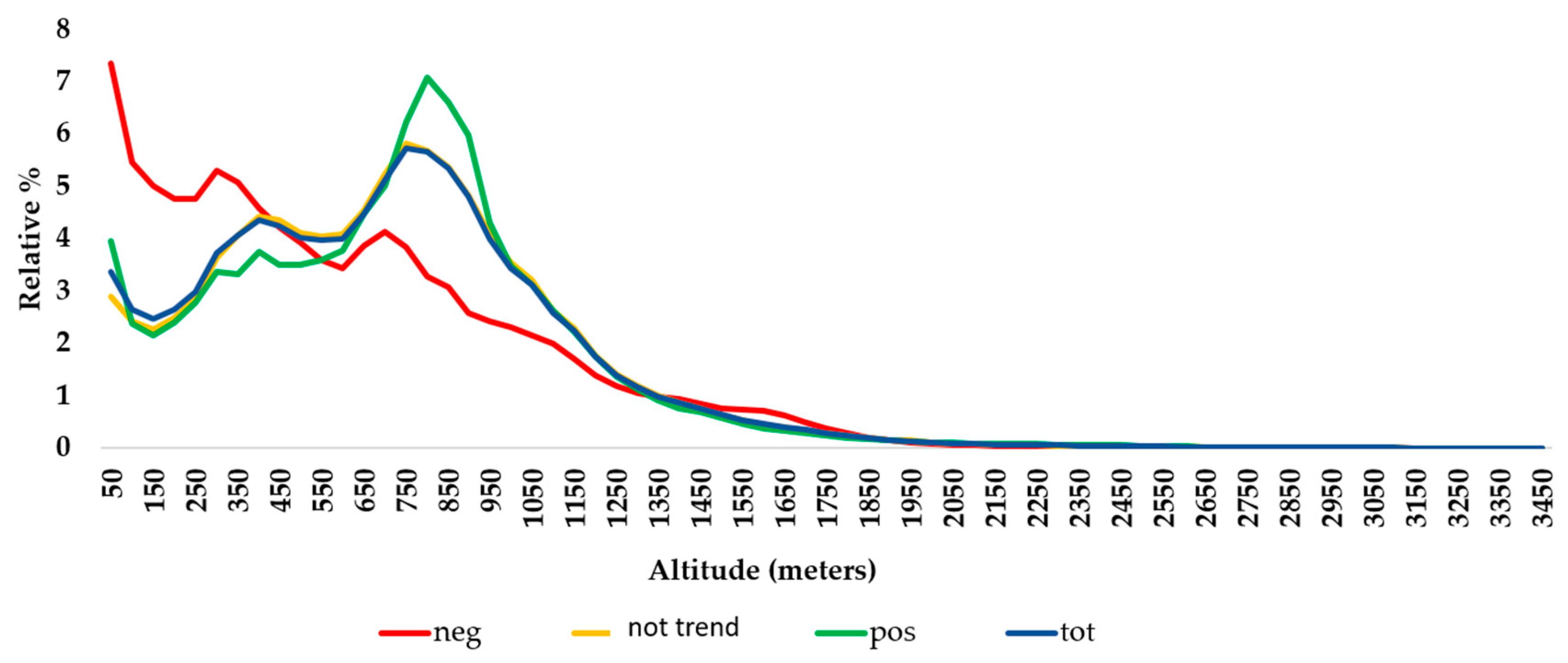
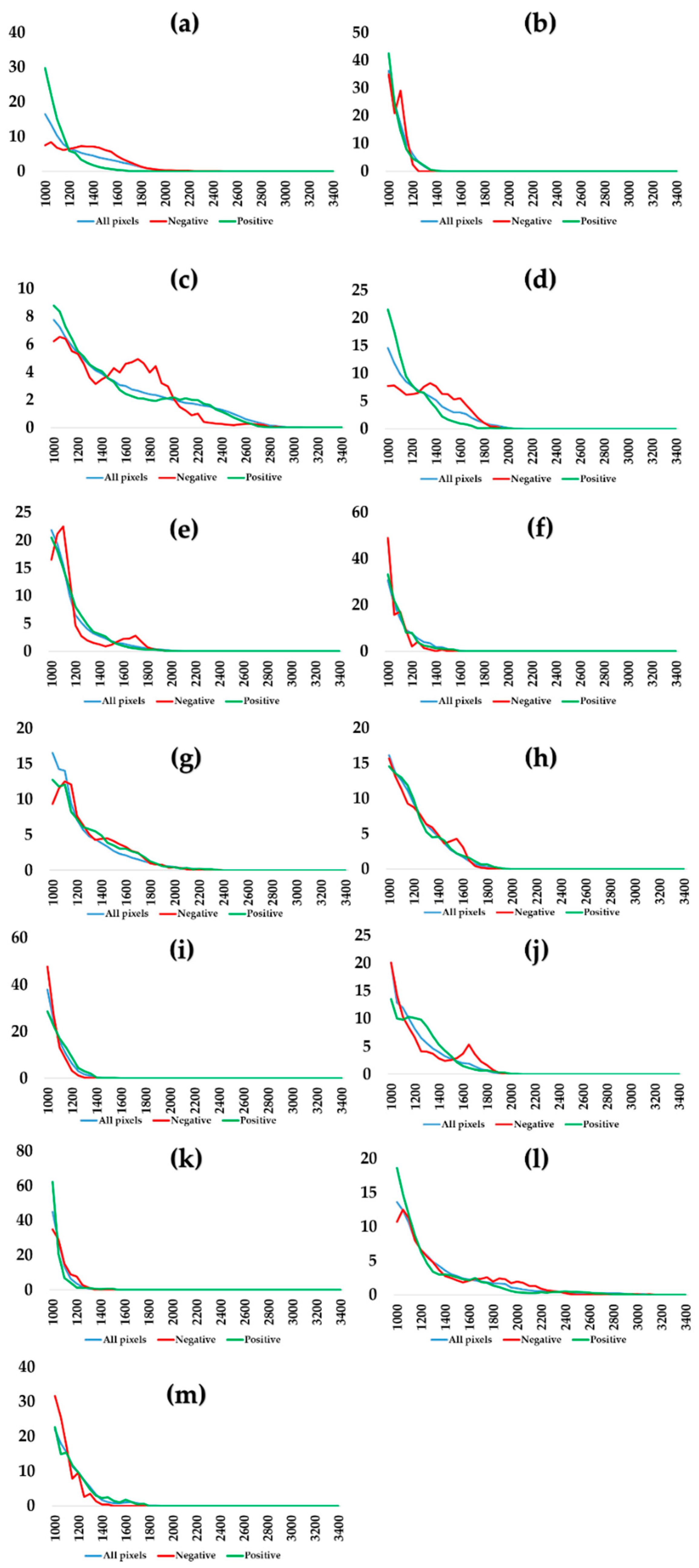
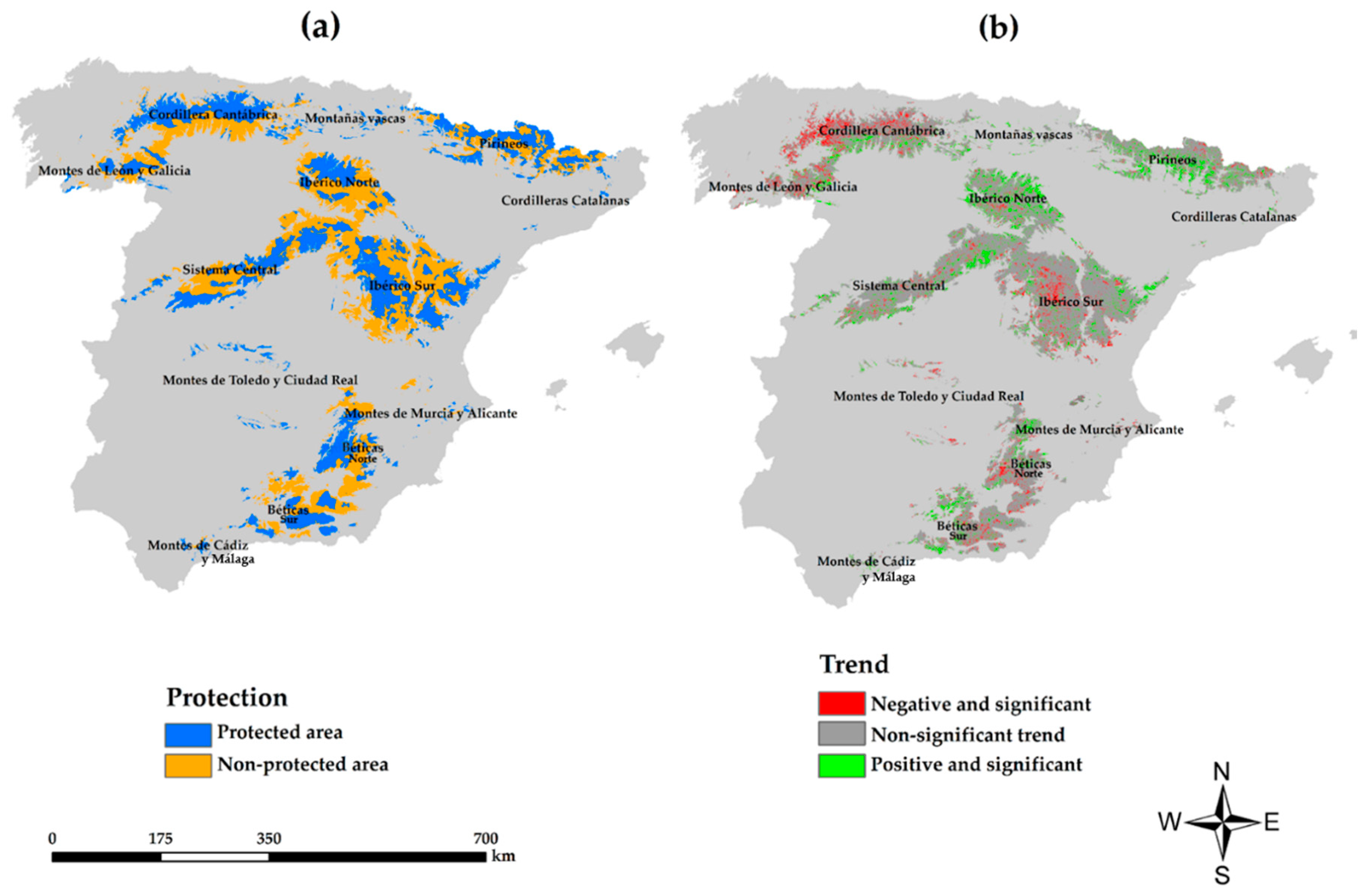
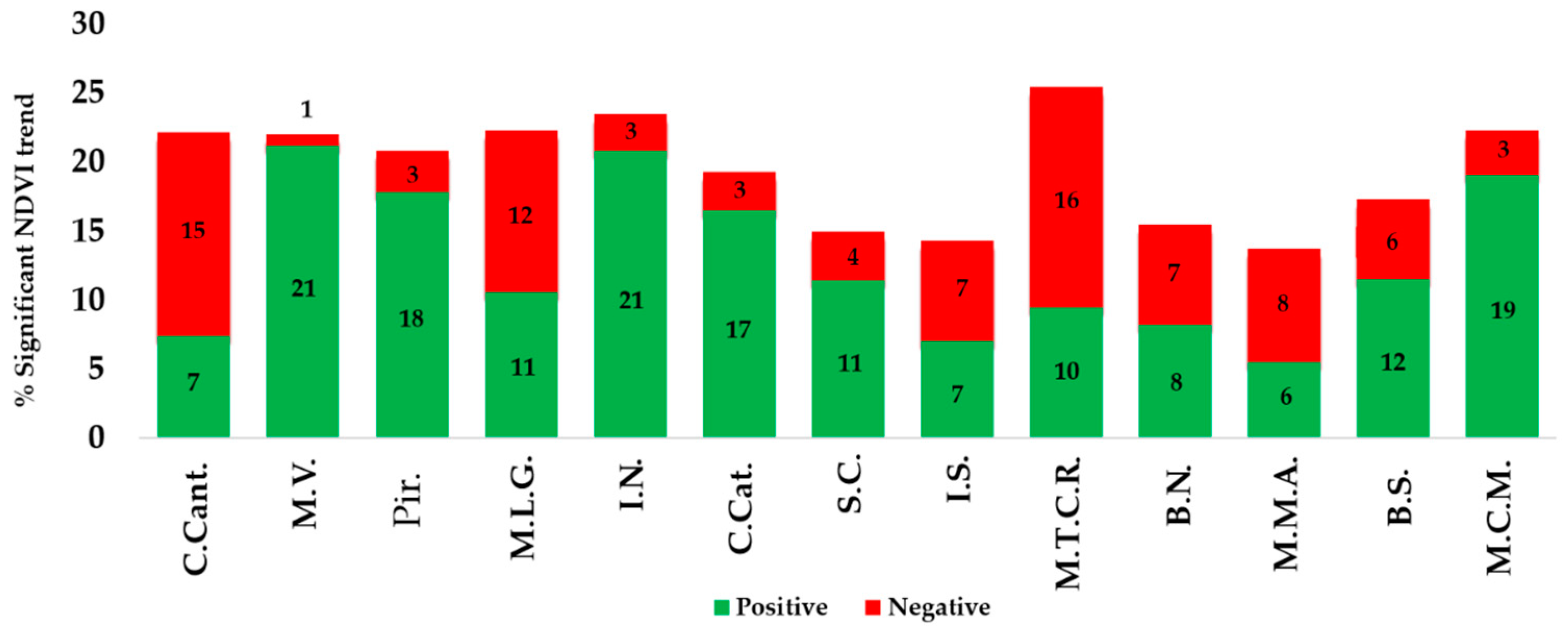
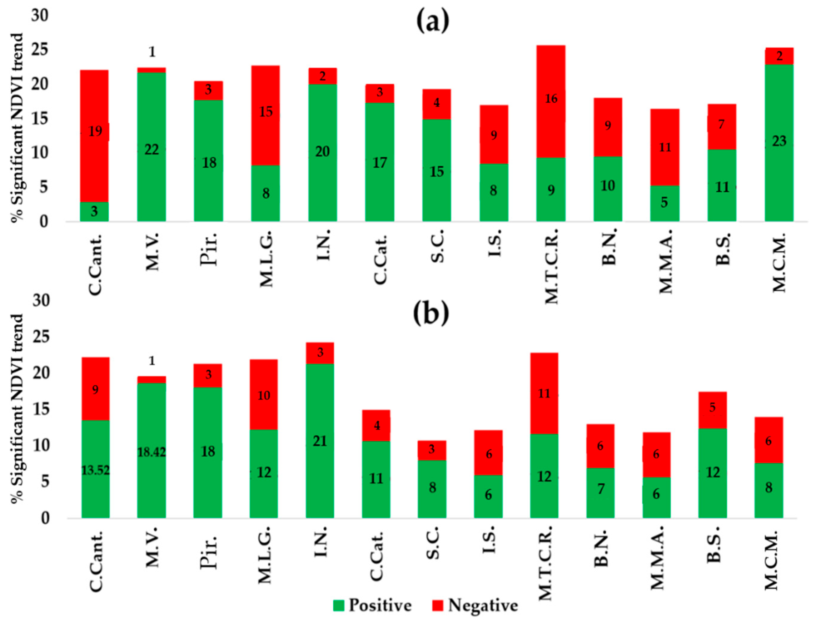
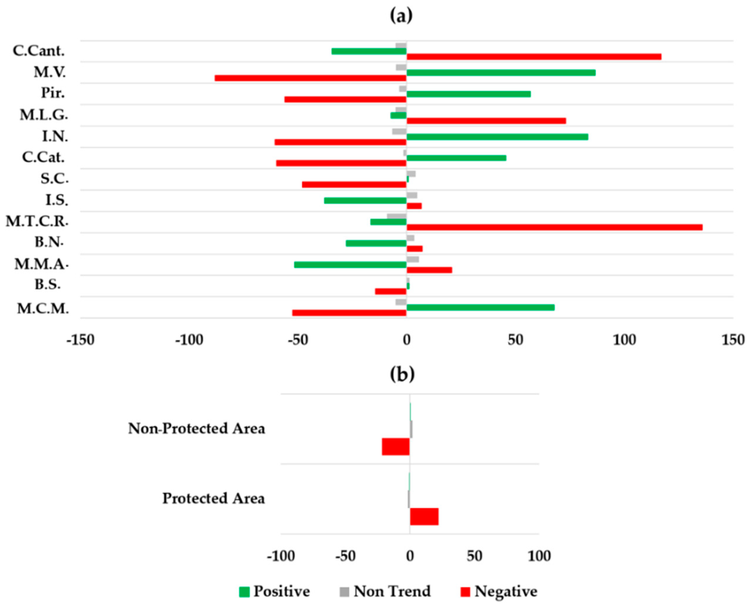
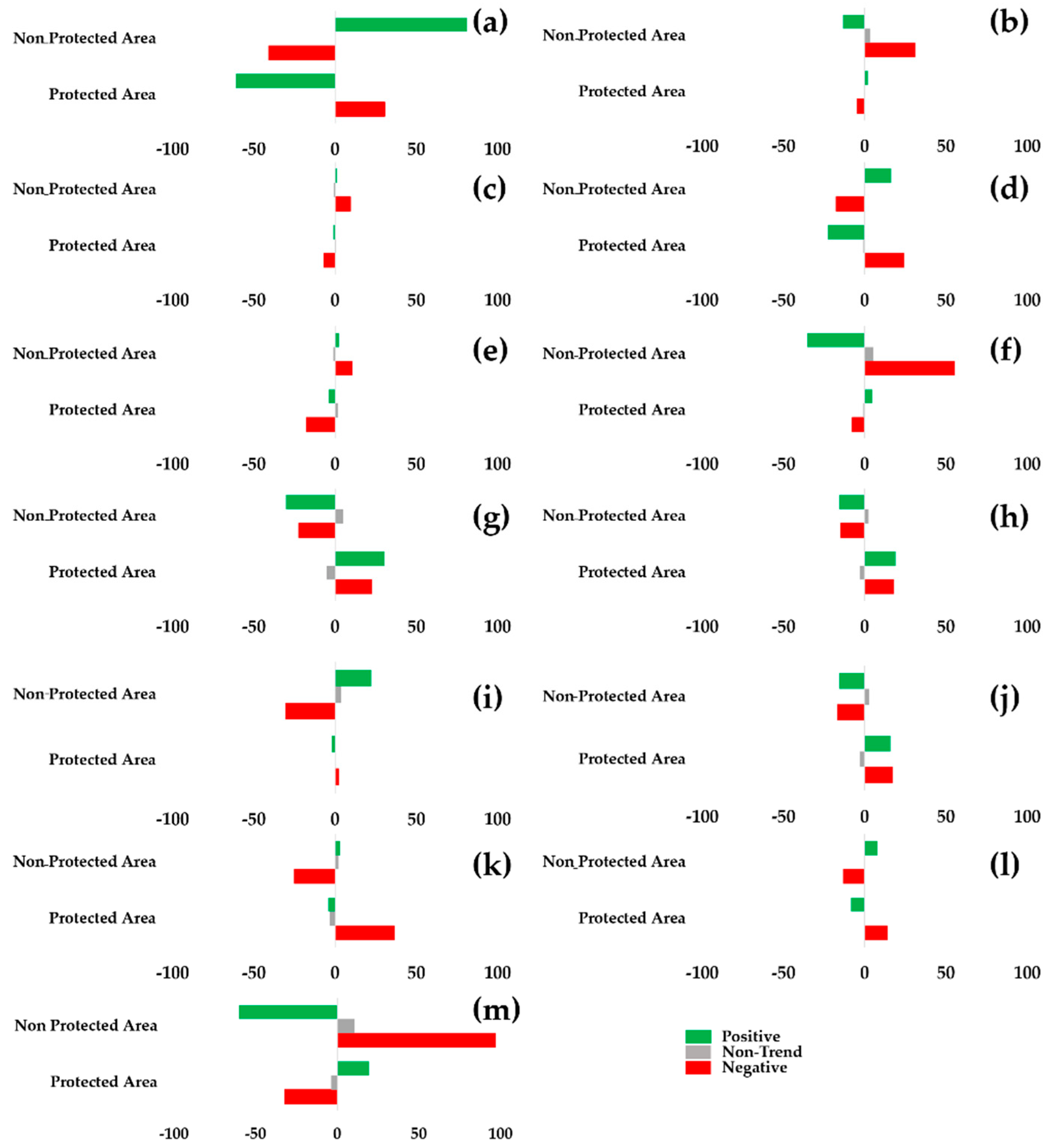
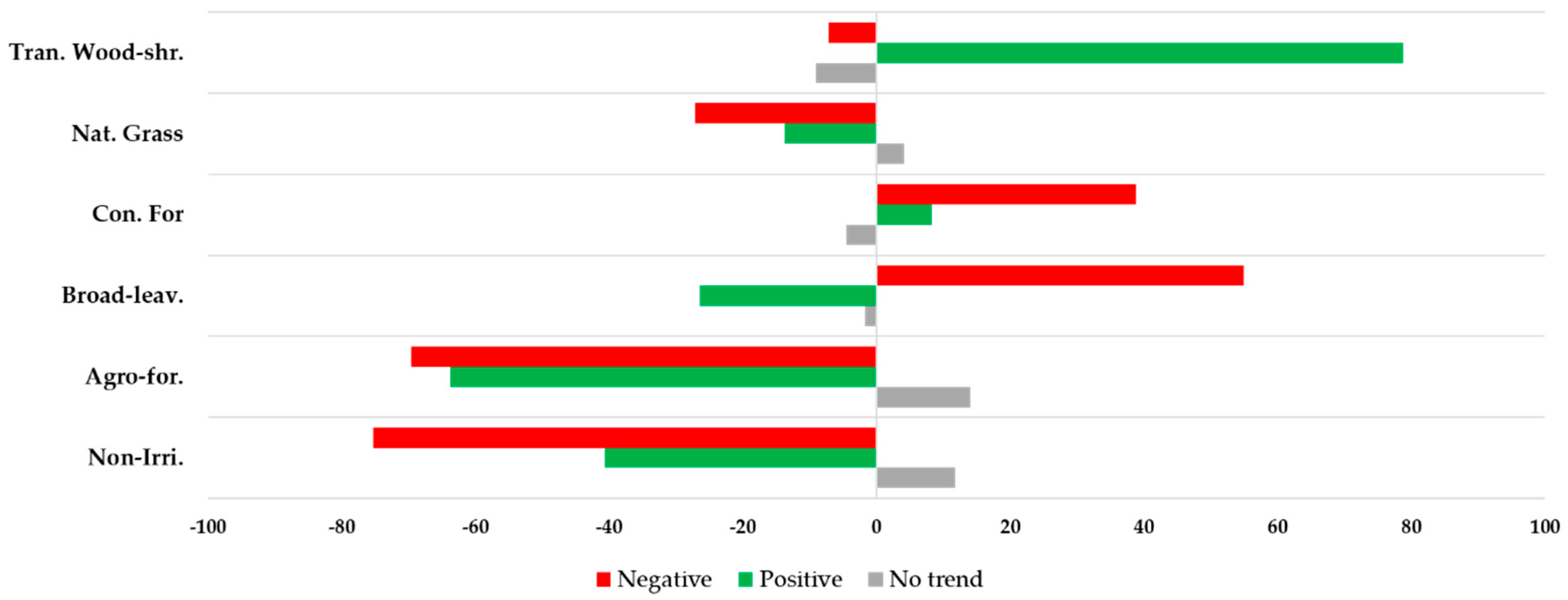
Table 1.
Mountain range characteristics.
| Mountain Name | Abbreviation | Protected Area | Area of Each Mountain (ha) | Height of Range (m) | Localization within Mainland Spain |
|---|---|---|---|---|---|
| Cordillera Cantábrica | C.Cant. | 57% | 1,407,436 | 2550 | North |
| Montañas Vascas | M.V. | 87% | 1,018,362 | 1500 | North |
| Pirineos | Pir. | 58% | 2,332,004 | 3350 | North |
| Montes de León y Galicia | M.L.G. | 42% | 797,456 | 2150 | North |
| Sistema Ibérico Norte | I.N. | 37% | 1,152,095 | 2300 | Continental |
| Cordilleras Catalanas | C.Cat. | 88% | 56,600 | 1650 | North |
| Sistema Central | S.C. | 50% | 1,277,718 | 2550 | Continental |
| Ibérico Sur | I.S. | 45% | 414,962 | 2000 | Continental |
| Montes de Toledo y Ciudad Real | M.T.C.R. | 42% | 85,842 | 1600 | Continental |
| Béticas Norte | B.N. | 50% | 778,615 | 2350 | South |
| Montes de Murcia y Alicante | M.M.A. | 41% | 38,408 | 1500 | South |
| Béticas Sur | B.S. | 48% | 44,295 | 3340 | South |
| Montes de Cádiz y Málaga | M.C.M. | 75% | 28,485 | 1500 | South |
Table 2.
Results from the chi-squared tests performed by mountains and the protected or not protected status of the area. * implies significance at 99% of CI. Abbreviations are reported in Table 1.
Table 2.
Results from the chi-squared tests performed by mountains and the protected or not protected status of the area. * implies significance at 99% of CI. Abbreviations are reported in Table 1.
| Data Used | V1 | V2 | Df | χ² | Sig. |
|---|---|---|---|---|---|
| All pixels | Trend | Mountain | 24 | 75,212 | * |
| All pixels | Trend | Protection | 2 | 6306 | * |
| C.Cant. | Trend | Protection | 2 | 13,603 | * |
| M.V. | Trend | Protection | 2 | 9 | * |
| Pir. | Trend | Protection | 2 | 52 | * |
| M.L.G. | Trend | Protection | 2 | 694 | * |
| I.N. | Trend | Protection | 2 | 156 | * |
| C.Cat. | Trend | Protection | 2 | 23 | * |
| S.C. | Trend | Protection | 2 | 3838 | * |
| I.S. | Trend | Protection | 2 | 2033 | * |
| M.T.C.R. | Trend | Protection | 2 | 26 | * |
| B.N. | Trend | Protection | 2 | 729 | * |
| M.M.A. | Trend | Protection | 2 | 65 | * |
| B.S. | Trend | Protection | 2 | 259 | * |
| M.C.M. | Trend | Protection | 2 | 281 | * |
Table 3.
Observed pure pixels by cover types within mountain areas in mainland Spain.
| Data Used | V1 | V2 | Df | χ² | p-Value |
|---|---|---|---|---|---|
| Pure pixels from the most representative land cover types | Trend | Cover type | 10 | 22,708 | <0.01 |
Table 4.
Area (ha) with significant trend and non-trend by cover types within mountain zones in Mainland Spain.
Table 4.
Area (ha) with significant trend and non-trend by cover types within mountain zones in Mainland Spain.
| Land Cover Name | Cover Type Acronym | Negative | Non-Trend | Positive | Total |
|---|---|---|---|---|---|
| Non-Irrigated arable land | Non-Irri. | 11,575 (2%) | 588,438 (92%) | 38,488 (6%) | 638,502 (100%) |
| Agro-forestry areas | Agro-for. | 628 (2%) | 26,483 (94%) | 1036 (4%) | 28,147 (100%) |
| Broad-leaved forest | Broad-leav. | 64,290 (11%) | 458,565 (82%) | 42,223 (7%) | 565,078 (100%) |
| Coniferous forest | Con. For. | 90,950 (10%) | 703,791 (79%) | 98,131 (11%) | 892,873 (100%) |
| Natural grasslands | Nat. Grass. | 23,285 (5%) | 374,225 (86%) | 38,215 (9%) | 435,724.91 (100%) |
| Transitional woodland-shrub | Tran. Wood-shr. | 35,741 (7%) | 393,357 (75%) | 95,190 (18%) | 524,288 (100%) |
| Total ha | 226,470 | 2,544,859 | 313,284 | 3,084,613 | |
| Total% | 7.00% | 83.00% | 10.00% | 100.00% |
Table 5.
Percentage of land cover change between 2000 and 2006 and between 2006 and 2012. Abbreviations are reported in Table 1.
Table 5.
Percentage of land cover change between 2000 and 2006 and between 2006 and 2012. Abbreviations are reported in Table 1.
| Mountains | % of Change 2000–2006 | Area (ha) of Change 2000–2006 | % of Change 2006–2012 | Area (ha) of Change 2006–2012 |
|---|---|---|---|---|
| C.Cant. | 0.109 | 10281 | 0.103 | 9715 |
| M.V. | 0.001 | 94 | 0 | 0.00 |
| Pir. | 0.025 | 2358 | 0.003 | 283 |
| M.L.G. | 0.239 | 22543 | 0.178 | 16,789 |
| I.N. | 0.049 | 4622 | 0.033 | 3113 |
| C.Cat. | 0 | 0.00 | 0 | 0.00 |
| S.C. | 0.133 | 12,545 | 0.112 | 10,564 |
| I.S. | 0.185 | 17,450 | 0.188 | 17,733 |
| M.T.C.R | 0.01 | 943 | 0.006 | 566 |
| B.N. | 0.043 | 4056 | 0.067 | 6320 |
| M.M.A. | 0.005 | 472 | 0.002 | 189 |
| B.S. | 0.093 | 8772 | 0.034 | 3207 |
| M.C.M. | 0.001 | 94 | 0.0001 | 9 |
| Σ | 0.893 | 84,230.25326 | 0.7261 | 68,487.77927 |
© 2018 by the authors. Licensee MDPI, Basel, Switzerland. This article is an open access article distributed under the terms and conditions of the Creative Commons Attribution (CC BY) license (http://creativecommons.org/licenses/by/4.0/).
Share and Cite
MDPI and ACS Style
Arrogante-Funes, P.; Novillo, C.J.; Romero-Calcerrada, R. Monitoring NDVI Inter-Annual Behavior in Mountain Areas of Mainland Spain (2001–2016). Sustainability 2018, 10, 4363. https://doi.org/10.3390/su10124363
AMA Style
Arrogante-Funes P, Novillo CJ, Romero-Calcerrada R. Monitoring NDVI Inter-Annual Behavior in Mountain Areas of Mainland Spain (2001–2016). Sustainability. 2018; 10(12):4363. https://doi.org/10.3390/su10124363
Chicago/Turabian StyleArrogante-Funes, Patricia, Carlos J. Novillo, and Raúl Romero-Calcerrada. 2018. "Monitoring NDVI Inter-Annual Behavior in Mountain Areas of Mainland Spain (2001–2016)" Sustainability 10, no. 12: 4363. https://doi.org/10.3390/su10124363
Note that from the first issue of 2016, this journal uses article numbers instead of page numbers. See further details here.