A Control Scheme for Variable-Speed Micro-Hydropower Plants


School of Electrical Engineering, Wuhan University, Wuhan 430072, China
*
Authors to whom correspondence should be addressed.
Sustainability 2018, 10(11), 4333; https://doi.org/10.3390/su10114333
Submission received: 24 October 2018
/
Revised: 14 November 2018
/
Accepted: 18 November 2018
/
Published: 21 November 2018
(This article belongs to the Section Energy Sustainability)
Abstract
:The aim of this work was to design and build a control system to control the performance of the Pelton wheel and synchronous generator system at different upstream water flow and electrical load conditions. The turbine output power is determined by the upstream water flow and spear valve, whilst the generator output power is determined by the turbine output power and the electrical load. A spear valve is used to control the generator output power at different water and load conditions. An autotuning proportion integration (PI) arithmetic-based controller was built using a relay feedback tuning method. An on–off relay was used in the program in order to oscillate the system. The optimal PI gains can be estimated via the Ziegler–Nichols method. A fully open test was used to test the tuned PI gains. The performance of the original gains and the new tuned gains were discussed. A controller was used to maintain the frequency or voltage of the output power by automatic regulation of the turbine valve. The program could search for the maximum generation efficiency by entering the output current value of the generator into the program manually.
1. Introduction
With the increasing rate of hydropower installation all over the world, there are many potential energy sources with low water heads that can be used by small-scale hydropower (SHP) plants to generate electricity for domestic use [1]. However, the overdevelopment of SHP may result in potential threats such as streamflow reductions [2]. These threats can be reduced through appropriately locating SHP plants in an environmentally friendly manner [3]. Furthermore, the operation mode of SHP plants can be used for variable renewable energy integration [4]. The ecological impacts of SHP still need to be thoroughly investigated; for instance, the impact on small river ecology [5].
During the last few years, rainfall patterns have changed erratically the world over [6]. Earth will enter a three-to-five-year drought period starting in 2018, which will occur inland at higher latitudes and in coastal areas at lower latitudes [7]. Due to these changes in rainfall patterns, the supply of water to a hydropower plant may vary with time. With the low investment and high return of small hydropower plants, many small hydropower stations have been attracted to invest in the construction of small hydropower stations [8]. Some basic design aspects of the micro-hydropower plant have been proposed in the literature [9,10,11]. A large number of the small hydropower stations have achieved grid-connected operation, which also puts forward new standards for the safe and effective operation of small hydropower stations [12].
The aim of this paper was to select a suitable water turbine and electrical generator combination to supply electricity to a grid of fixed voltage. The generator, driven by the turbine, operates at variable speed, and hence with varying voltage and frequency. The variable outputs were to be regulated by the power electronics. For a permanent magnet synchronous generator, an algorithm is proposed to increase the system efficiency via optimizing the rotation rate [13]. A novel electronic power conditioning system is built for increasing the efficacy of SHP [14]. An induction generator can be used instead of a synchronous generator in a SHP plant for its size and cost benefits [15]. In this paper, the aim was to design and build a control system to control the performance of the Pelton wheel and synchronous generator system at different upstream water flow and electrical load conditions. A feedback control structure was implemented to control the system. The aim was to have two different results from controlling the turbine. The first was to apply different loads to the electrical generator (simulating different levels of electricity usage) while keeping the system at a constant frequency. The second was to apply different upstream flows (simulating different water level conditions) while keeping the system at the maximum efficiency possible (varying frequency).
2. Materials and Methods
2.1. Overview of the Control Section
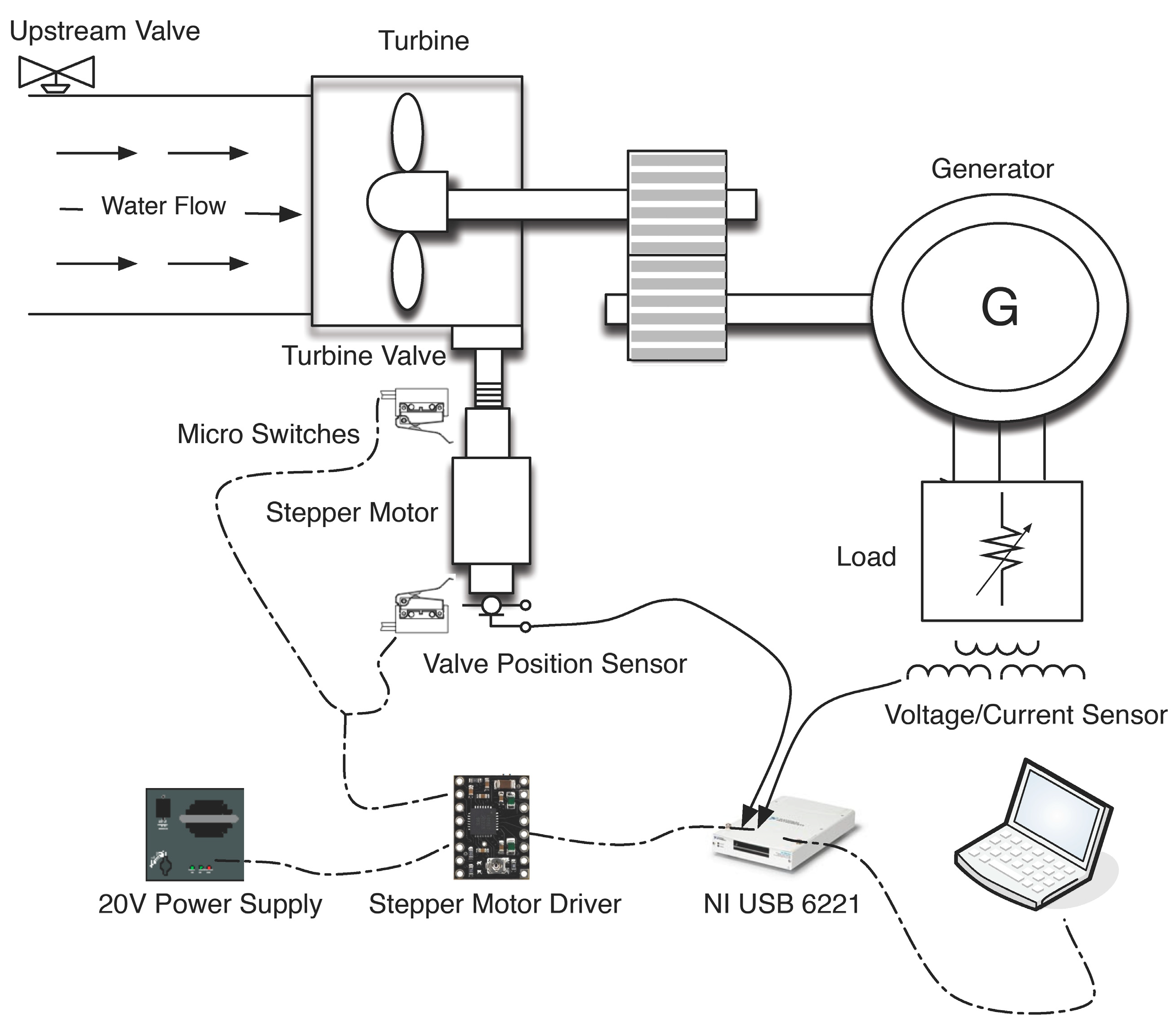
This section of the variable-speed hydropower scheme describes the design of a control system using LabVIEW (Laboratory Virtual Instrument Engineering Workbench). A schematic diagram of the power generator is shown in Figure 1. A water tank (32 m head) within the University of Leicester was used to produce water flow in order to drive a turbine. The generator could extract electrical power while the turbine was rotating. A resistance load was connected to the end of the generator in order to receive the electrical power.
The motion controller was a stepper motor. The stepper motor could be used to change the characteristics of the turbine via a valve. At different water conditions, the control of the valve position could be used to adjust the turbine characteristics for maximum efficiency and the required power output. The position of the valve was controlled by the NI-USB 6221 card (National Instruments-Universal Serial Bus 6221). The card was used to acquire data from the sensors and generate signals to control the stepper motor via a stepper motor driver. A personal computer was used to control the card using LabVIEW.
2.2. LabVIEW and Data Acquisition
LabVIEW uses a graphical programming language. The graphical user interface (GUI) can accelerate programming, as the programming process involves drawing a flowchart. LabVIEW programming can generally be twice as fast compared to C and C++ [16]. Moreover, a high-performance control and monitoring system can be built using this programming language. The LabVIEW software is designed for measurement, data analysis, and motion control. A number of built-in underlying codes designed by National Instruments can be called from the toolset of LabVIEW for signal processing [16].
A NI-USB 6221 multifunction data acquisition (DAQ) board, as shown in Table 1, can be used to acquire and/or generate analog/digital signals. The input signals are translated from analog signals to digital signals for computer processing. Afterwards, the processed signals can be translated to analog control signals using the data acquisition card. The LabVIEW software can be used to design the core control gain K of the control system, as shown in Figure 2.
2.3. Method of Autotuning Proportion Integration (PI) Control
2.3.1. Autotuning the PI Control
A PI control is a feedback control used to increase the control of performance. Stability is a crucial consideration in the control design. A feedback control is necessary when the system includes [17]:
- Uncertain signal because of unknown disturbance;
- Uncertain models;
- An unstable plant.
In the variable-speed hydropower project, the upstream water flow is hard to predict exactly, and the generator is difficult to model accurately. Therefore, a proportion integration differentiation (PID) control can be used to increase the control performance. A normal PID can be expressed as:
For a discrete-time control system, is the discrete-time control signal:
where is the control signal, is the proportional gain, is the integral gain, is the derivative gain, (min) is the integral time, (min) is the derivative time, and e is the control error.
Autotuning is a process of setting optimal PID gains and applying them to the controller automatically. The proportional parameter P is used to increase the control response speed; the integral gain is used to adjust the oscillations. The increase of integral gain can be used to reduce the steady-state error, but can increase the overshoot. The derivative parameter D can be used to control sudden changes, but can increase the measurement noise. The derivative time is normally set to zero, since the D gain often decreases the performance of a controller [18].
2.3.2. Ziegler-Nichols Method
The Ziegler–Nichols method is an algorithm used to work out optimal PID parameters. This method involves setting the I and D parameters to zero first and increasing the proportional gain until the control response is oscillating [18]. The critical proportional gain and oscillation time are and (min), respectively. Lastly, the new PID gain can be adjusted as shown in Table 2 [19].
2.3.3. Relay Feedback Tuning
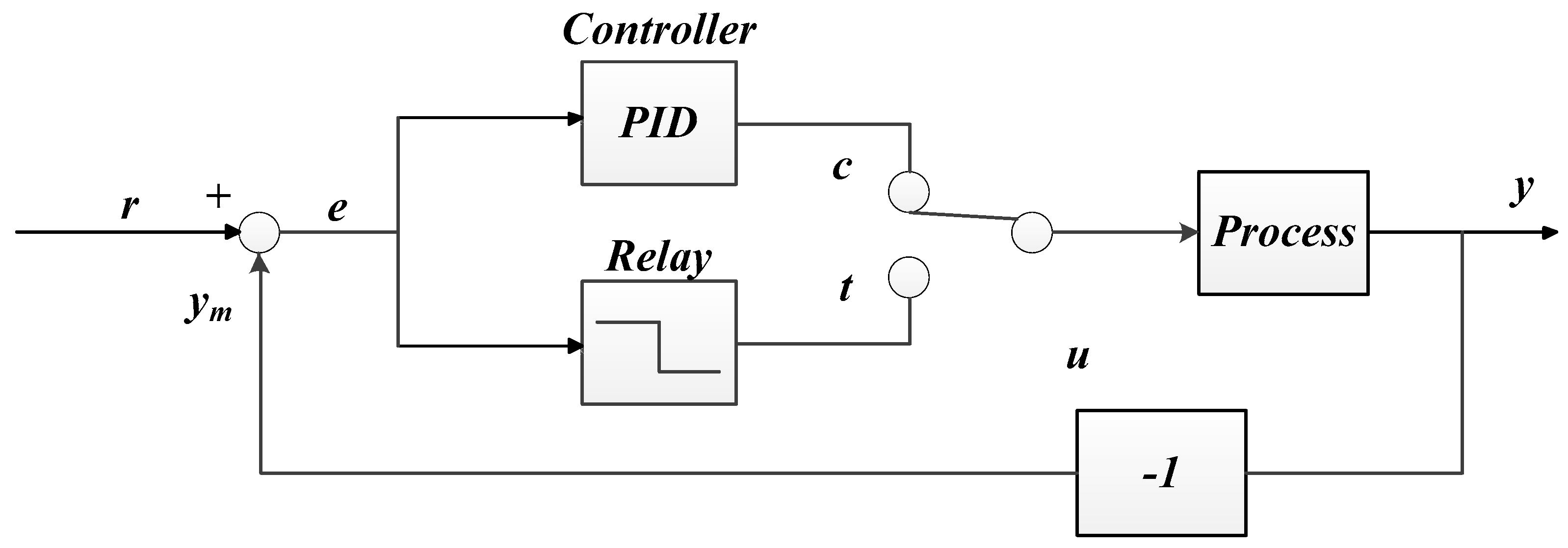
The relay autotuning technique is an algorithm to determine ultimate PID gains automatically. Åström and Hägglund reported this technique [20]. This method is based on the Ziegler-Nichols frequency domain design formula. It is hard to automatize the Ziegler-Nichols experiments; therefore, an on–off relay is used in the feedback loop in order to calculate ultimate gains using the relay experiments as shown in Figure 3.
The system can be operated as an autotuning or a normal PID controller while the switch connects to t or c, respectively. A relay control can lead to large phase delay at high frequencies. A phase lag of over 180° at sufficient frequencies can lead to oscillation with a period [12]. Therefore, a critical PID can be obtained from the feedback loop with the relay. In the autotuning mode, the period of the error e is equal to the oscillation period . The Fourier series can be used to work out the frequency domain waveforms. The amplitude of the first harmonic of the relay output can be expressed as:
For ,
where d is the relay amplitude and is the amplitude of the first harmonic of the relay output.
Therefore, the critical gain of the process can be expressed as:
where is the relay amplitude and is the output of the process.
This relay experiment gives the critical proportional gain and oscillation time (min). A new PID can be calculated using the Ziegler-Nichols method.
3. Experimental Preparation
3.1. LabVIEW Program
The entire program was designed using LabVIEW 2013. Several of the toolkits designed by National Instruments are required in order to use their sub-VIs (virtual instruments). The program may not run without the following requirements:
- LabVIEW 2013: Any other version of LabVIEW may support the program; however, new buttons in the 2013 version were used in the front panel. The old versions may indicate a different user interface.
- NI-DAQmx 9.5.5: The DAQmx is the basic drive software designed by National Instruments in order to achieve PC-based data acquisition.
- DAQ assist: This sub-VI is required for communication between the DAQ hardware and the LabVIEW software.
- National Instrument LabVIEW PID and Fuzzy Logic Toolkit: This toolkit is required to integrate PI and autotuning control algorithms into the LabVIEW programs.
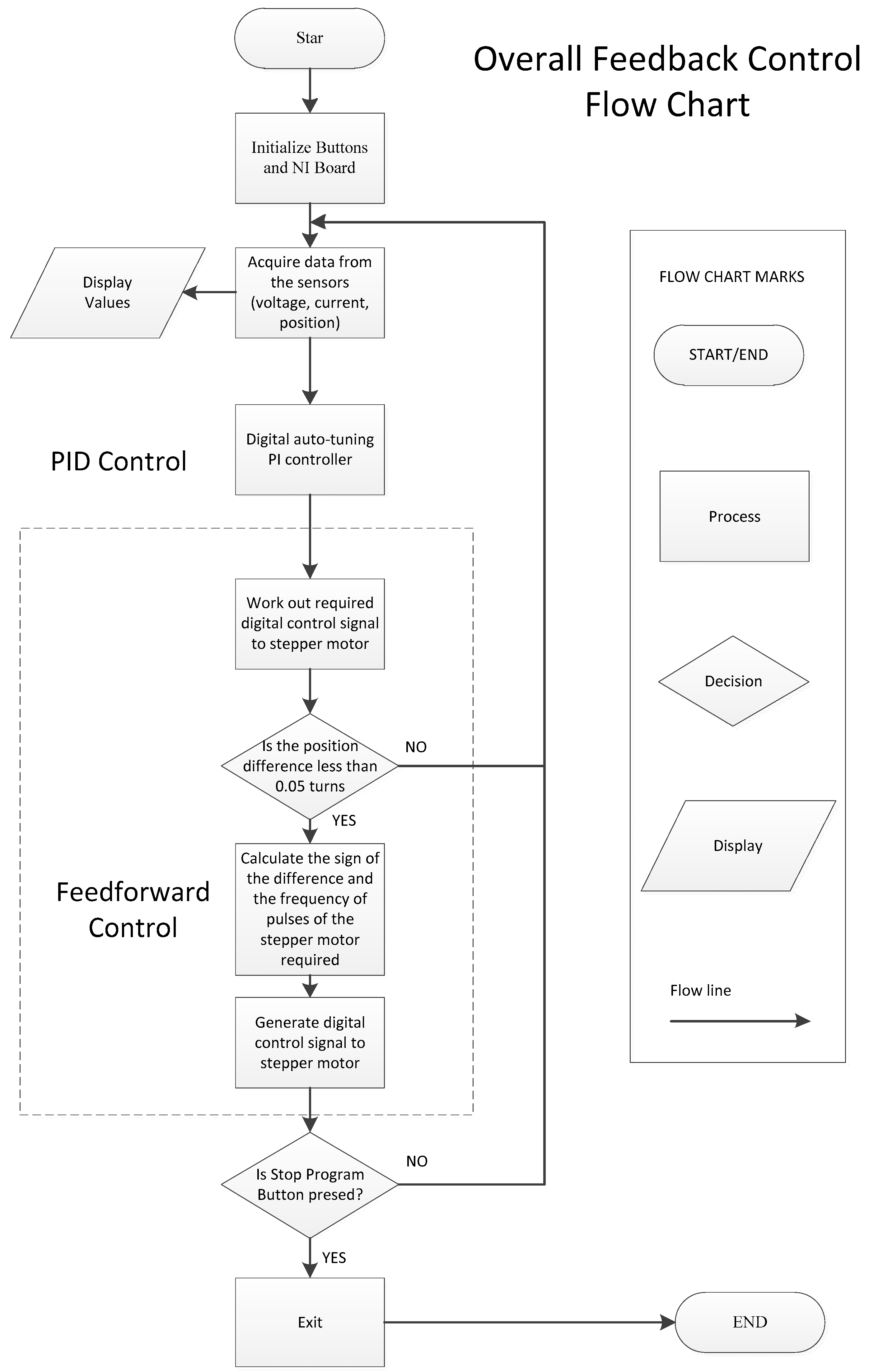
The overall LabVIEW program follows the flow chart shown in Figure 4.
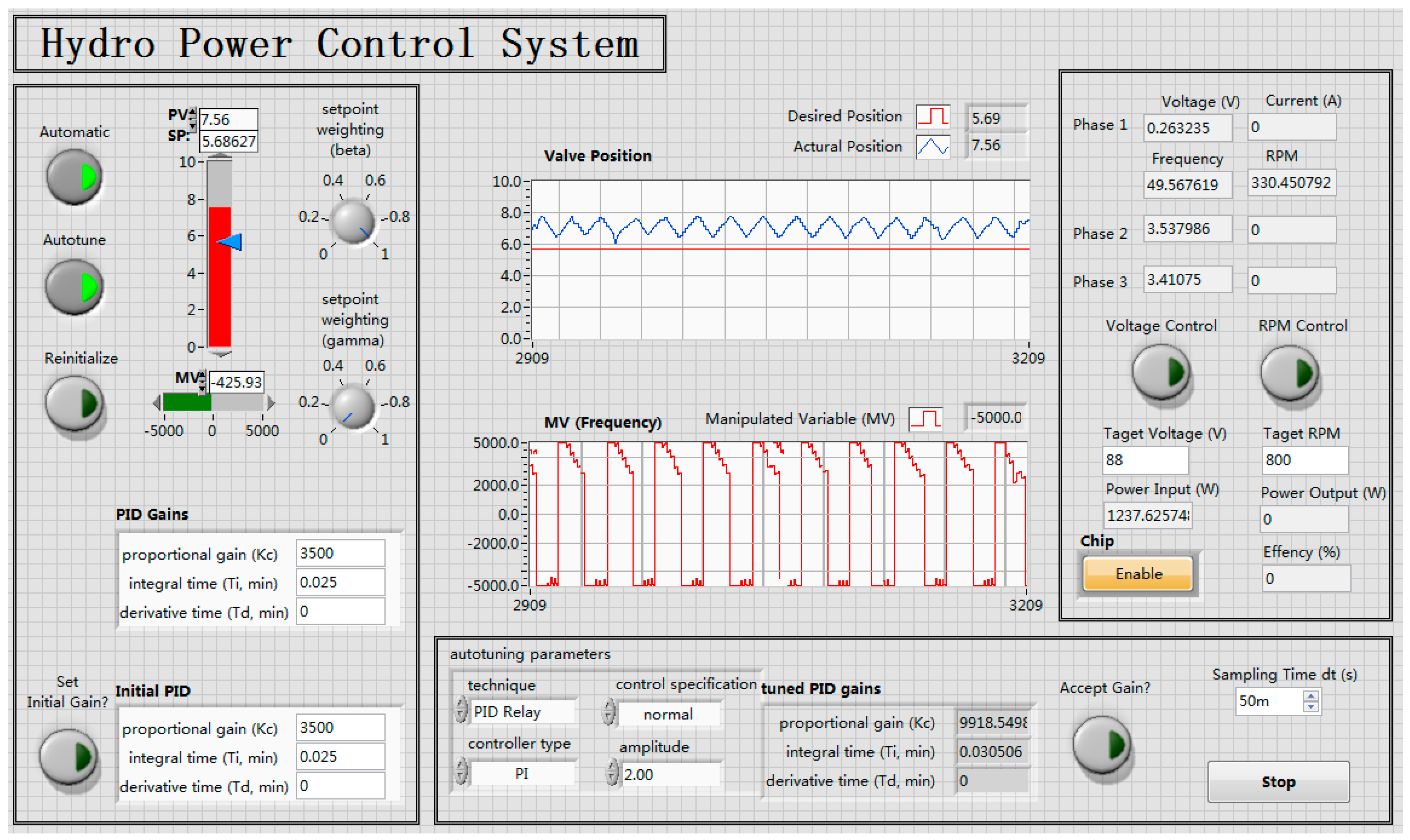
3.1.1. Front Panel
Figure 5 shows a screenshot of the front panel of the hydropower control system VI. All the elements were labeled to enable easy operation by the user. There were three main blocks and two waveform indicators in the front panel. The left block was used to design the PI controller. The buttons can be used to start the automatic PID control (Automatic), start the autotuning algorithms (Autotune), set the initial PID parameters (Set Initial Gain), and reinitialize the PID parameters (Reinitialize). The bottom block was used to design the autotuning experiment parameters. The results of experimental PID gains were shown in the indicator (tuned PID gains) and can be applied to the controller when the Accept Gain? button is pressed. The right block was used to indicate the power output and set the target voltage or RPM (revolutions per minute) in order to maintain the output voltage or RPM. The turbine valve position (desired and actual) versus time was plotted in the valve position indicator. Meanwhile, the frequency of the output pulse signal was recorded in the manipulated variable indicator.
3.1.2. Block Diagrams
The block diagram includes three w loops operating in parallel. The three loops were used to process data, generate pulses, and provide autotuning control.
The data processing loop, as shown in Figure 6, was used to acquire data and display results. A DAQ assistant was used to acquire the data from the sensors. Local variables created for the data were required to be delivered between the different loops.
The turbine valve position was indicated using the voltage measured from the potentiometer. The 0–5 volt signal measured from the potentiometer was multiplied by 2 in order to represent 0–10 turns of the valve. The actual and the desired (autotuning control loop) valve positions were bundled together and indicated in one waveform graph. As a result, the differences between the actual and desired valve positions can be shown on the front panel.
The turbine output power was indicated using an experienced formula. Different upstream flows controlled by an upstream valve were used to simulate different water level conditions. The turbine output power was tested every half turn, from one half-turn open (0.5 turns) to fully open (10 turns). A third polynomial was used for curve fitting to ensure the calculated output power was accurate to ±5%. From the established formula, the turbine output power can be calculated from the valve position:
where Pout (W) is the power output from the turbine and t (turns) is the valve position of the upstream flow, ranging from 0.5 to 10.
A Fourier transform was used to acquire the frequency of the signal. The voltage signals were translated from the time domain to the frequency domain. A low pass filter (0–200 Hz) was used to remove high-frequency noise. Meanwhile, the effective value of the signal could be calculated according to the frequency.
The revolutions per minute of the generator were acquired using the frequency of the power. Since the speed of the synchronous (permanent magnet) generator is directly related to speed through the number of pole pairs of the generator, the RPM is equal to the frequency multiplied by 60/9. Since the frequencies of the three phases are equal, the RPM of the generator can be acquired from only one phase. There are two ways to measure the frequency: The first method is to directly measure one phase frequency from a voltage/current sensor. The second method is to measure the frequency of a power sensor. As the current would be multiplied by the voltage signal using a multiplying circuit, one phase frequency can be acquired from the multiplied signal. The frequency of the power sensor is double that of the voltage/current sensor, as shown by Equation (4). The voltage and current have the same frequency. The total power output is the sum of the three phases.
where (W) is the power consumption, i (A) is the load current, Im (A) is the maximum of the load current, (Hz) is the load current angular frequency, and I (A) is the effective valve of the load current.
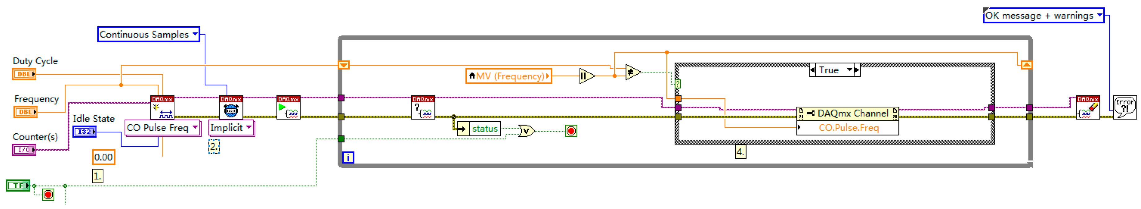
The pulse generation loop, as shown in Figure 7, was used to generate a continuous pulse to drive the stepper motor. The frequency is a local variable using the PID controller result. A generator of a continuous digital pulse, train.vi, was used to communicate between the LabVIEW and the DAQ board.
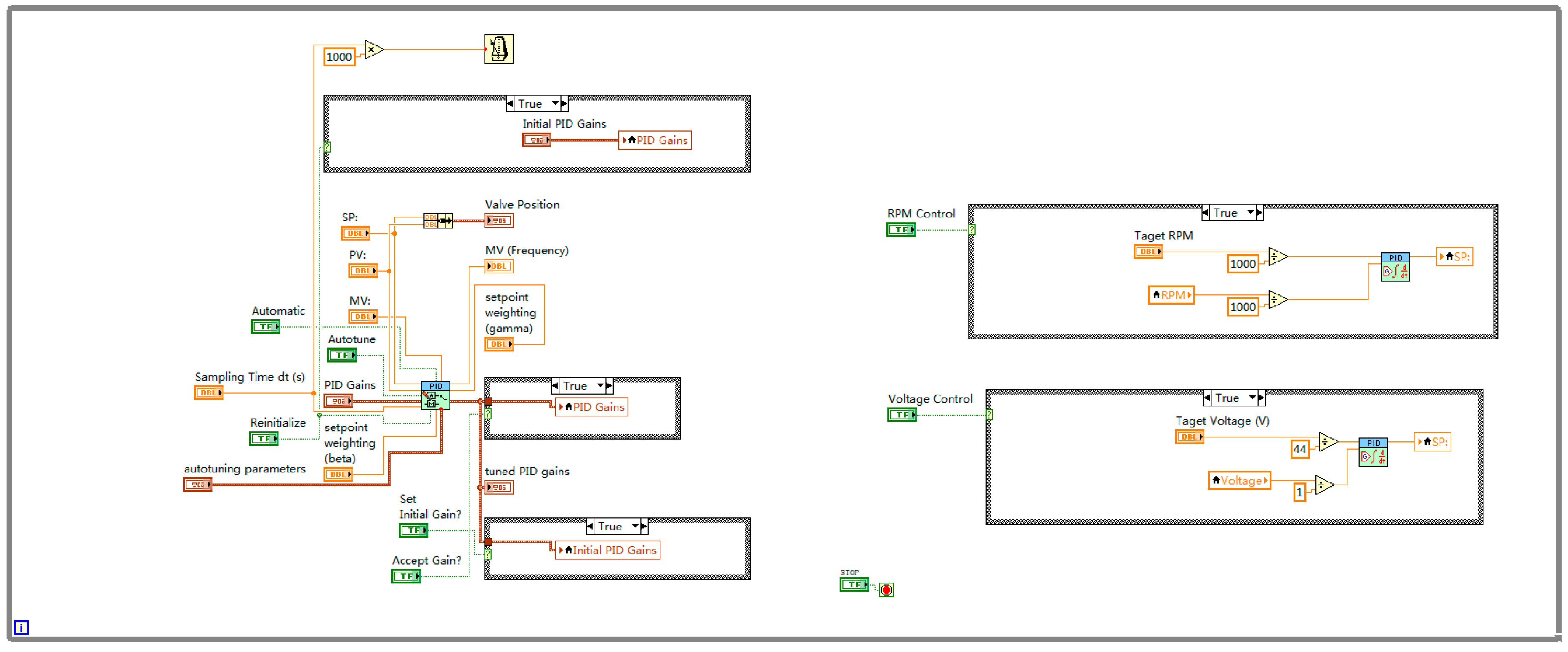
The autotuning control loop, as shown in Figure 8, was used to set optimal PID gains automatically. A PID.vi was used to calculate the optimal PID gains using the autotuning algorithms. The delay of the loop is the sampling time of the PID algorithms. Hence, the program can acquire signals continuously.
Two “if” loops were used to achieve maintained frequency and voltage functions, as shown in Figure 9. Boolean buttons were used to activate “if” loops in order to control the frequency or voltage. Both the frequency and voltage control used an extra PID controller to work out the setpoint of the valve. The control system was complex in this situation. The integral and derivative gains were set to zero in order to avoid uncontrolled uncertainties.
3.2. Experimental Apparatus
A schematic diagram of the power generator is shown in Figure 10. A stepper motor was used to control the valve of the turbine in order to control the power input into the generator.
3.2.1. Stepper Motor
The choice of the stepper motor was based on the requirements of the mechanical mates. The torque requirement of the stepper motor was 1.4 Nm in order to drive the valve. Meanwhile, a double-shaft stepper motor was required, since a potentiometer was required to be installed at the back. Hence, an OMEGA double-shaft stepper motor (OMHT23-400) was used to control the valve. The rated torque was 1.86 Nm. The step angle was 1.8°, and therefore 200 step signals were required for one revolution. A bipolar stepper motor driver was required as the motor has two pairs of windings.
3.2.2. Stepper Motor Driver
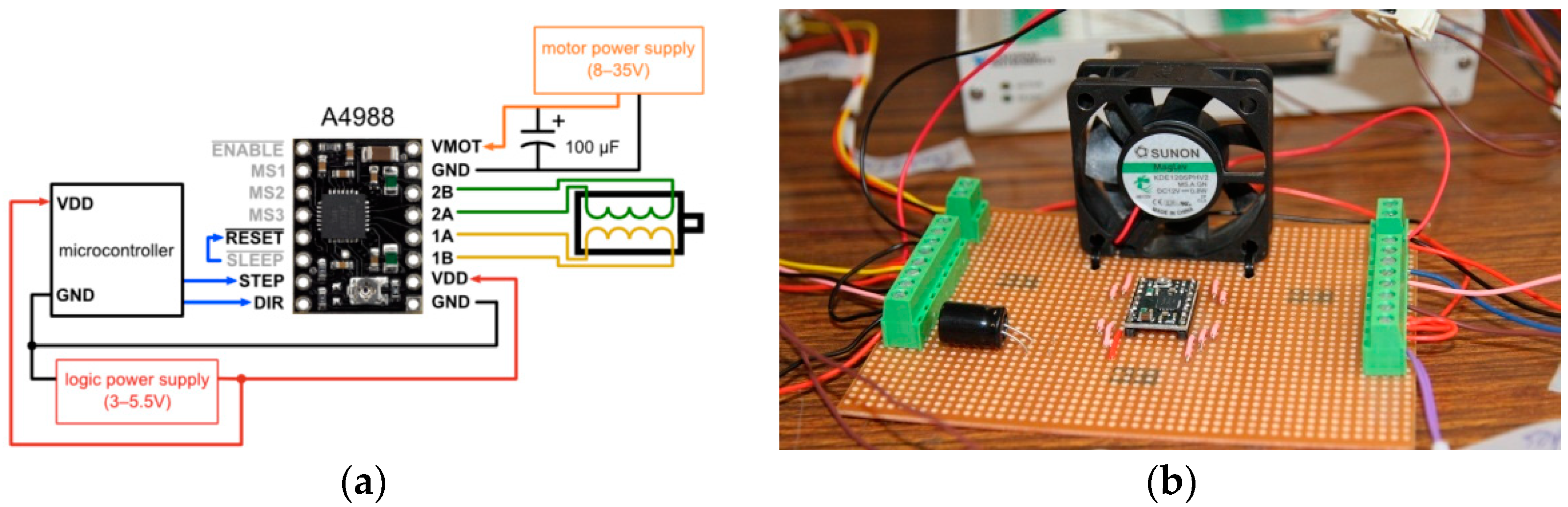
An A4988 bipolar stepper motor driver was used to drive the stepper motor, as shown in Figure 11. It can deliver up to 2 A per coil with sufficient additional cooling. The A4988 board can be permanently damaged when the input voltage exceeds 35 V. A 100 µF capacitor was connected across motor drive voltage (VMOT) and ground (GND) in order to protect against possible spikes from the power supply. A power supply was connected across the VMOT and GND to provide power to drive the stepper motor. The device drive voltage (VDD) and ground (GND) were connected to the power supply of the NI-DAQ board to acquire logical circuit power. The step (STEP) and direction (DIR) were connected to the NI-DAQ board to receive pulse trains and direction commands, respectively. The outputs of the board (1A, 2A, 1B, and 2B) were used to drive the stepper motor. The microstep (MS) pins were used to set microstep resolution, as shown in Table 3. “Half Step” means two pulse signals were required in order to drive each step angle.
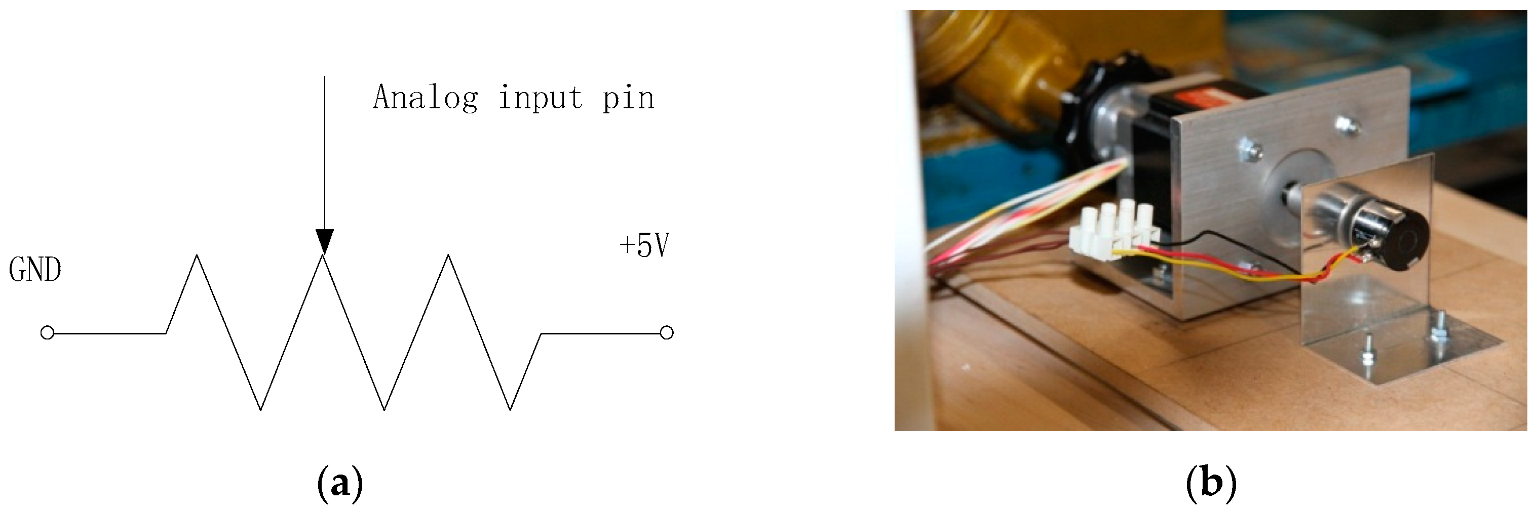
3.2.3. Potentiometer
A potentiometer is a variable resistor with three ends, as shown in Figure 12. The potentiometer can be used to produce variable potentials from the analog input pin end. The other two ends were connected to two different potentials, and therefore the slid end potential can be varied between these two potentials.
A ten-turn potentiometer was used to indicate the valve position via the variable potentials. The variable potentials were between 0 V and +5 V, since the two ends were connected to the ground and +5 V source, respectively. A change of one turn anticlockwise of the potentiometer can lead to 0.5-V increases of the slid potential.
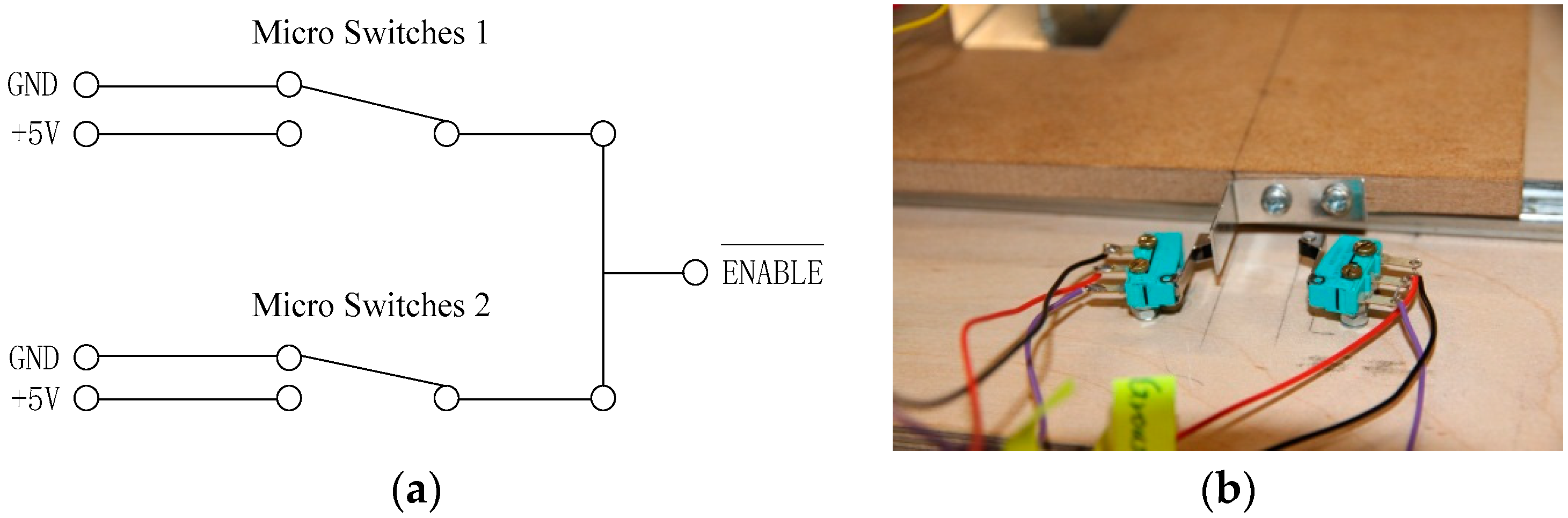
3.2.4. Micro Switches
Two micro switches were used to build an emergency system, shown in Figure 13. The emergency system can stop the stepper motor immediately if the frame moves out of the safety range. The safety range was larger than that of the software, since the hardware emergency system should be only activated after failure of the software protection.
The micro switches were single-pole double-throw switches. The input terminals were connected to the ground and +5 V sources. The output terminals were connected to the pin of the stepper motor driver. The driver was enabled when the pin was set to low. Hence, the driver would stop generating a pulse signal when either of the switches was closed. Meanwhile, the holding torque of the stepper motor was used to stop the inertia.
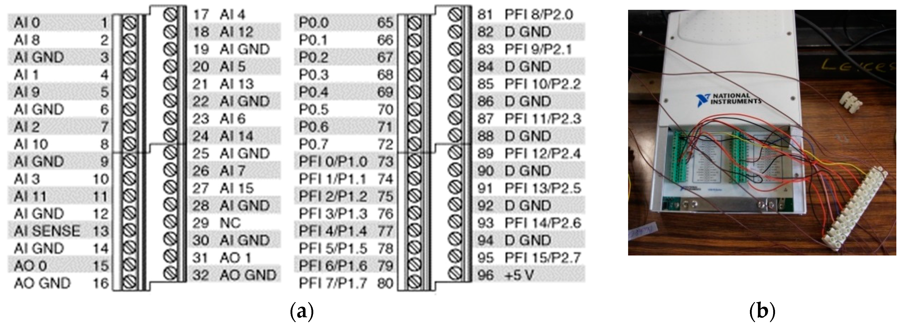
3.2.5. NI-DAQ Board
A NI-DAQ board was used generate/acquire signals, as shown in Figure 14. It had 8 channels of differential analogue input (16 single-ended), 2 of analogue output, and 2 time to live input/output (TTL i/o) ports of 8 lines each. All the wires were organized using an intergraded terminal in order to avoid unexpected short circuiting. The AI and AO stand for analog input and analog output, whilst the P and PFI stand for port and front-panel line, respectively. The analog inputs were used to acquire analog voltage signals from the sensors. The ports were used to switch between low logic and high logic in order to control the motor direction and driver state. The front-panel line was used to generate digital pulse trains from the hardware counter. The hardware counter can produce digital pulse trains of superior accuracy at high frequency. The pulse trains were used to provide step amounts to drive a stepper motor.
4. Results and Discussion
4.1. PI Gain-Tuning Experiment
PI gain-tuning experiments were applied before any PI controls were introduced. The experiment was used to work out the optimal PI gains for controlling the valve. As there is a lot of backlash in this system, the tuning experiment was conducted under maximum upstream flow in order to obtain conservative gains. The PI tuning experiment used an on-off relay to oscillate the control system. From the turbine characterization, the maximum efficiency only occurred between the valve positions 4–8 (6–8 for large upstream flow). The PI tuning experiment was oscillating the system around the position 6.5, since these valve positions would be used frequently. The program started the autotuning after the Autotune button was pressed. The valve was oscillated between positions 6 and 8 with an amplitude of 2. The actual position line shows that the valve position varied with time. The desired position line does not show anything in the autotuning mode. The oscillation time was recorded by the program, and an optimal PI gain was calculated using the relay feedback algorithm.
The PI gains were applied to the controller after the tuning experiment. The tuned PI gains were indicated at the bottom of the front panel. The user can review the new gains before applying them into the system in order to avoid unrealistic gains. The new gains can be applied after the Accept Gain? button is pressed, as shown in Figure 15. The proportional gain was increased from 3500 to 9918.5, whilst the integral time was increased from 0.0250 to 0.0305 min. After the new gains had been applied to the system, the Autotune button was released in order to operate the system in the PI control mode, as shown in Figure 16. The new gains can be set as initial gains when the Set Initial Gain? button is pressed. The control system can be operated using the initial gains when the Reinitialize button is pressed.
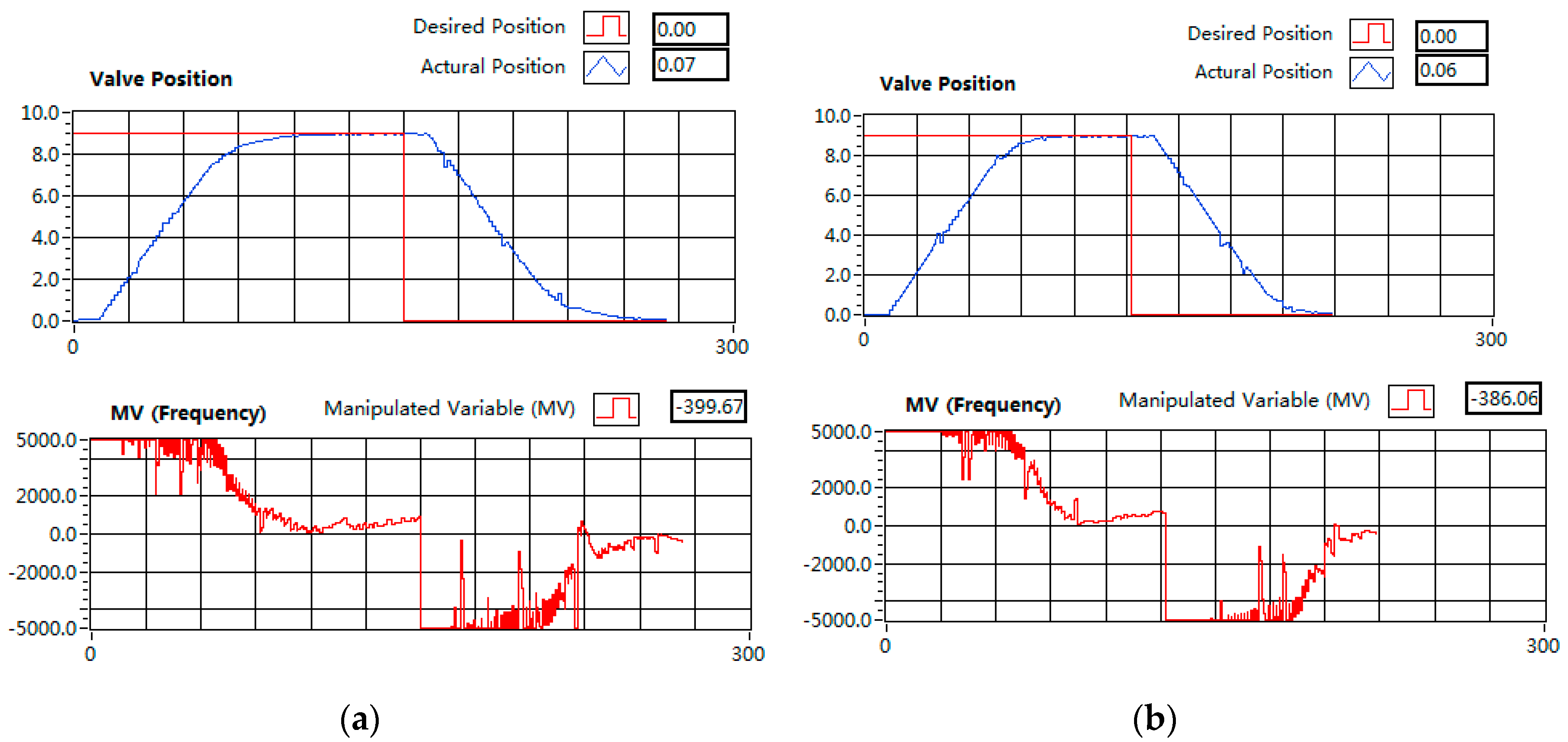
The performance of the new gains was tested using a manual control. The valve was turned to position 0 as the initial position. The desired initial position was position 9. The program started to record the valve position after the LabVIEW start button was pressed. The desired position was set to position 0 after the actual position reached a steady state. The rise time can be read from the waveform as shown in Figure 17. The scale of the time axis was 2.5 s. The new PI gains can perform with a faster response than the original PI gains. As the maximum pulse frequency was limited by the motor operating characteristics, both these two PI gains control systems had little position overshoot. The actual valve position had a 1.5-second delay, which is called dead time. The dead time can be caused by the slow response of the stepper motor and the delay of the position sensor. The potentiometer had negligible delay since the resistor cannot produce delay. Hence, the delay of the system response came from the slow response of the stepper motor. The torque of the stepper motor inversely varied in the RPM to some extent when the input power was constant. The low start torque at high-frequency pulses can lead to the low response of the stepper motor. The inductance in the winding also required time to respond to the current. The new PI gains were good since the valve was operated from a fully closed to fully opened state within ten seconds, and vice versa.
4.2. PI Control Experiment
4.2.1. Frequency and RPM Control
The hydropower control system can maintain the RPM and frequency at different upstream water flow and electrical load conditions. An RPM controller was used to control the frequency of the output power. In the synchronous generator, the speed was directly related to the speed: 333 RPM corresponds to 50 Hz. Since the electrical mates did not have a AC-DC-AC (or AC-AC/AC-DC) circuit to maintain the frequency of the output power, it was essential to maintain the frequency.
It was impossible to reach the frequency of the output power of 50 Hz while using the maximum upstream flow. The turbine output power can be estimated using the valve position, as introduced in Equation (7). The valve should be turned to around position 1 to obtain a 50 Hz power output. However, the power input of the turbine was increased dramatically around position 1. It was difficult for the valve control system to reach such an accurate point as the noise of the potentiometer is too large in the small control range. Moreover, the turbine output power was variable at an extremely small valve position while being connected to the generator with a resistance load.
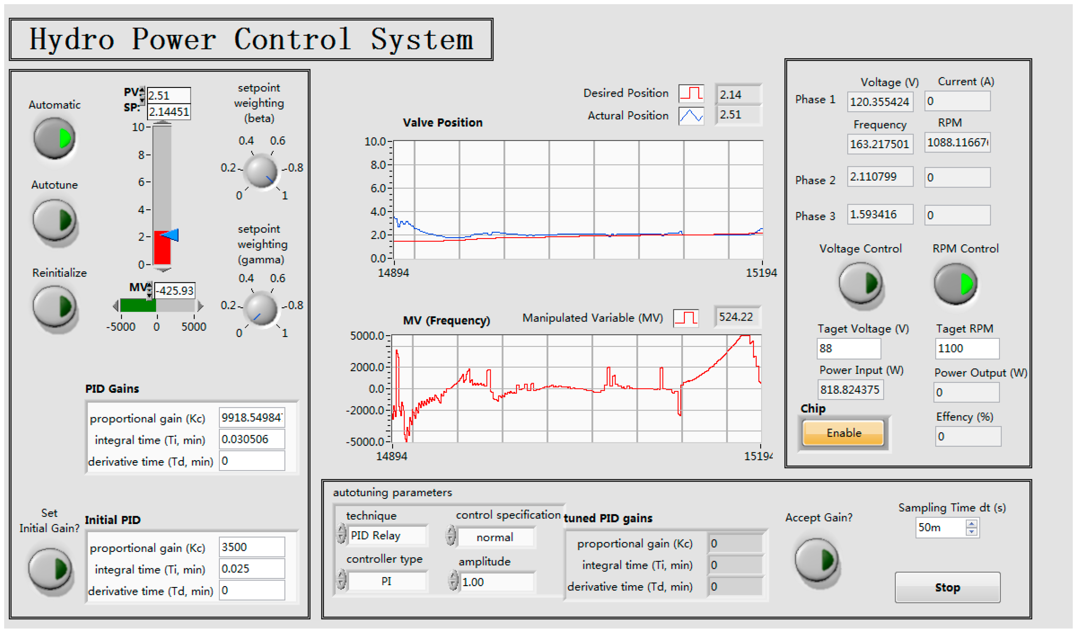
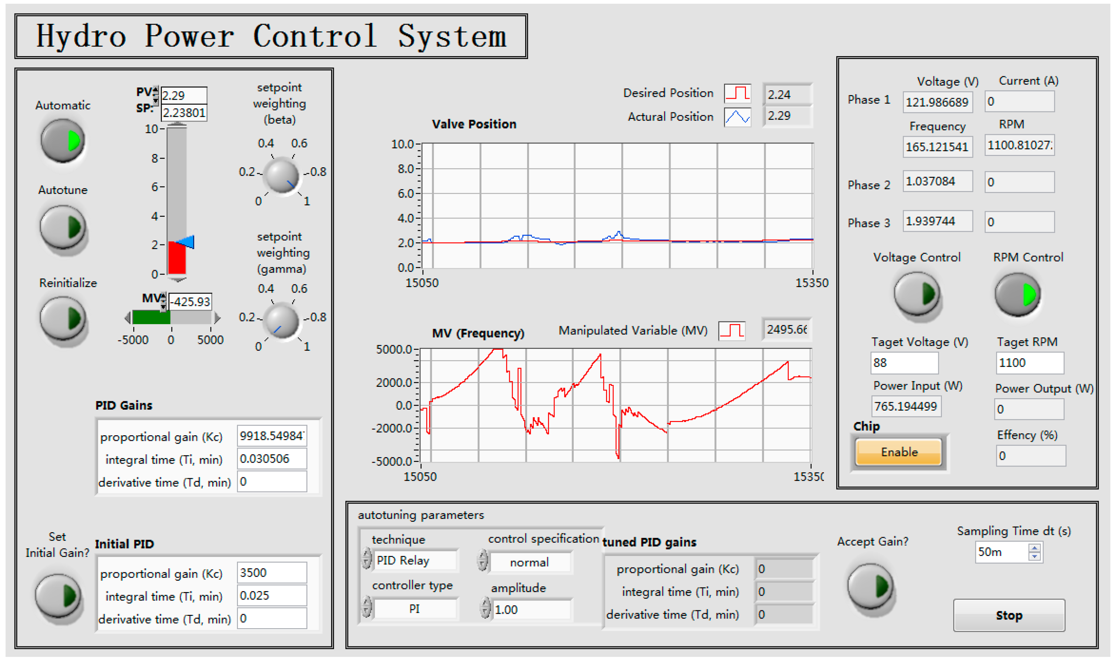
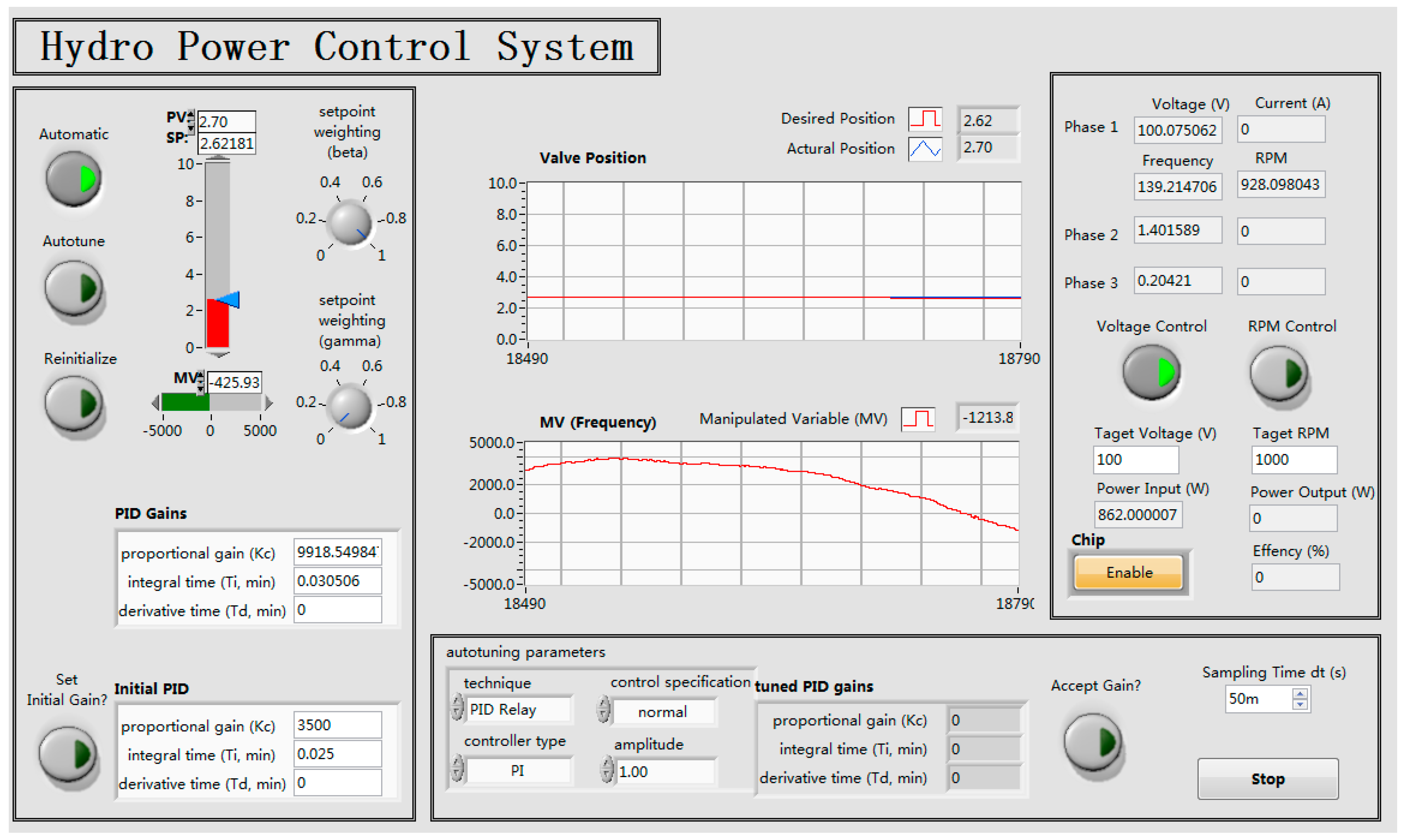
The control system can maintain the RPM at 1100. Figure 18 shows the operation interface screenshot before the RPM control was introduced. Here, the RPM was at 1088, which was close to the target of 1100 RPM. After the RPM control button was pressed, the stepper motor changed the valve from position 2.51 to 2.29, and the RPM reached the target value of 1100. However, this does not imply that the RPM was increased when the valve position was turned to a lower position. This can be caused by the shaking that occurs during turbine operation. Since the actual position in the program is measured by the potentiometer, the potentiometer might not measure the position accurately. The system was oscillating as the program received differently measured feedback at the same valve positions. The oscillation was the steady-state error and can be reduced from the integral gain of the controller. Fortunately, the accuracy of the voltage sensor cannot be changed by the shaking of the turbine. Hence, the measured RPM value was reliable.
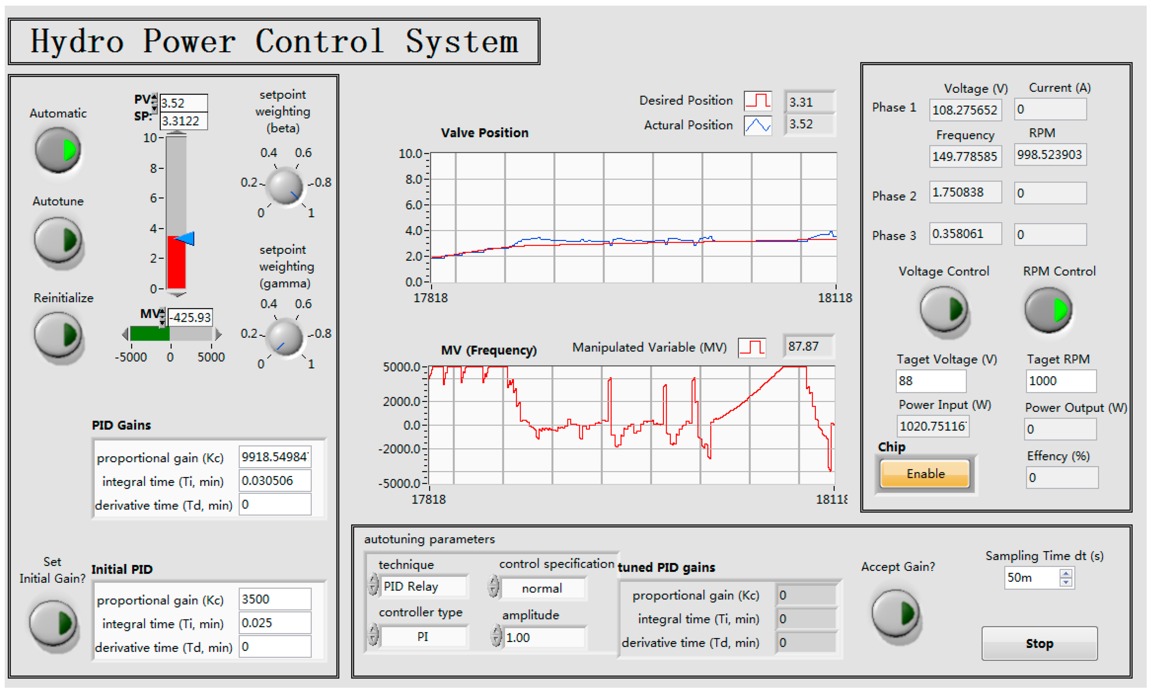
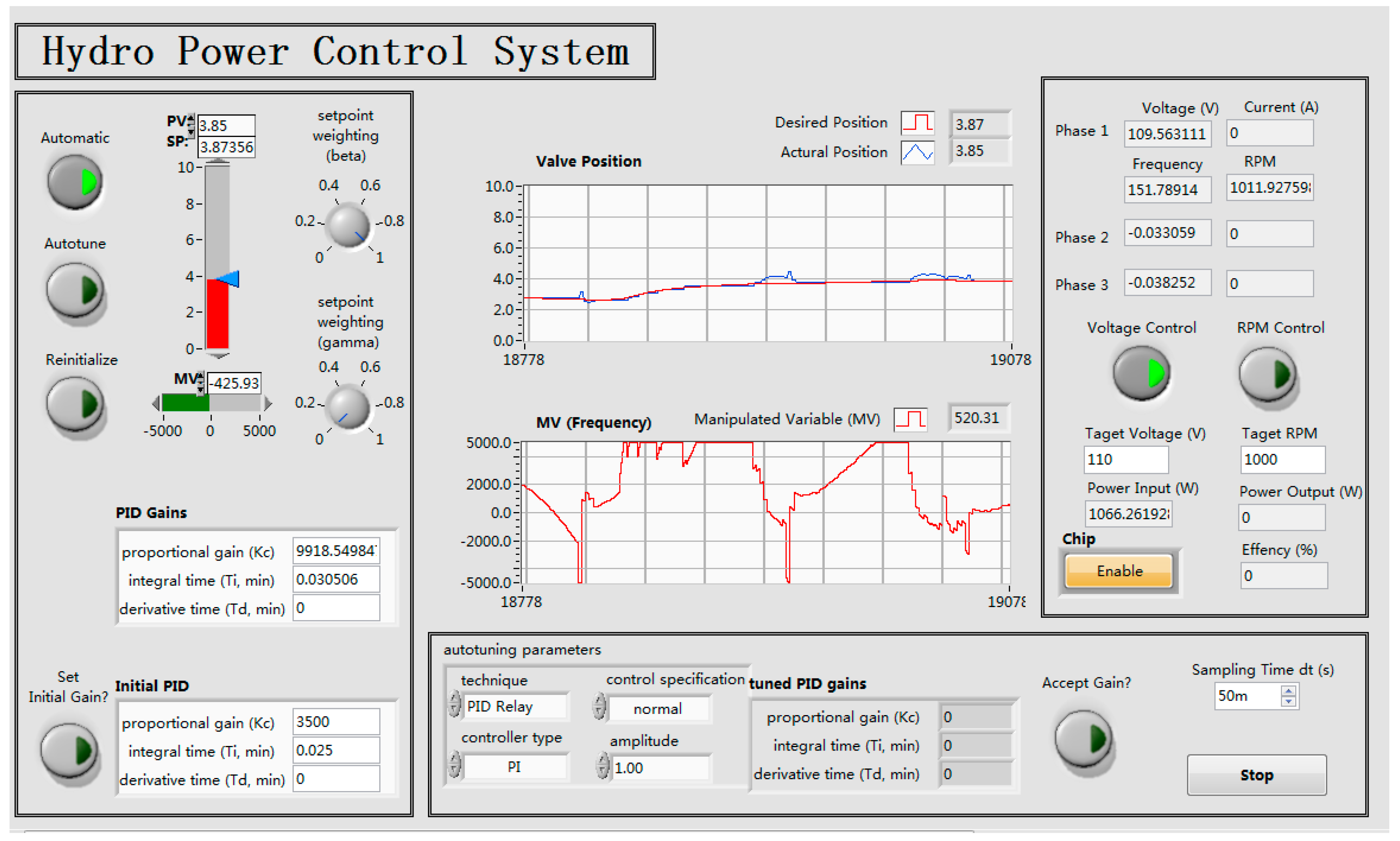
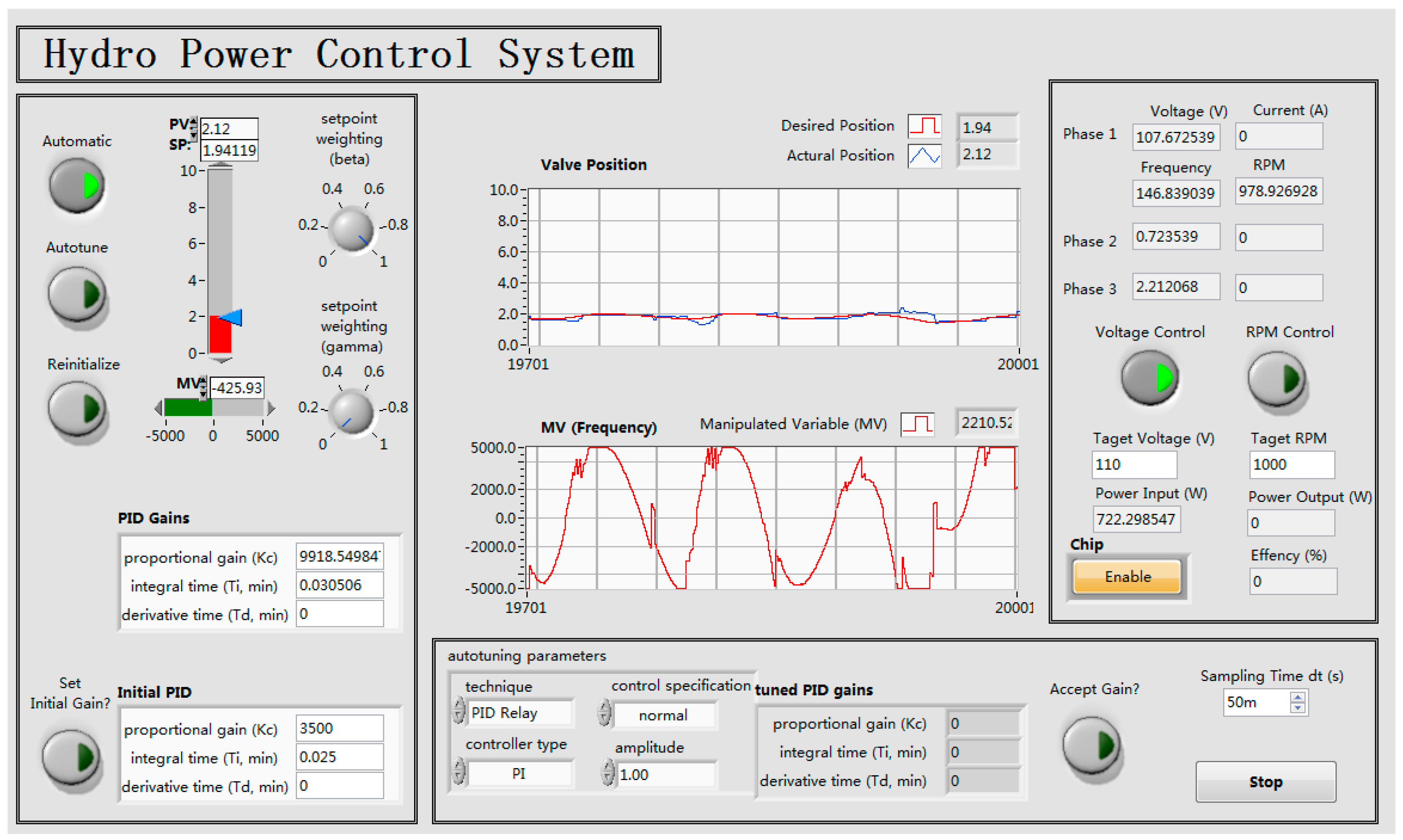
The target RPM was changed from 1100, as shown in Figure 19, to 1000, as shown in Figure 20. Since the program cannot obtain a valve position able to reach the target of 1000 RPM, the load was increased from 220 to 110 Ω. Afterwards, the voltage was dropped from 121 to 108 V when the valve position was changed from position 2.29 to 3.25.
4.2.2. Voltage Control
The control system can maintain the voltage under different load and upstream water flow conditions. Since the electrical mates only have a 50–60 Hz current sensor, the LabVIEW program cannot obtain the output current of the generator. The efficiency of the overall system can be calculated by dividing the power input by the power output of the generator. The power input can be estimated from Equation (7), and the voltage output can be measured from the voltage sensor. However, the 50–60 Hz current sensor was designed for the output of an AC-DC-AC (AC-AC) circuit (also not appropriate in this context). The sensors cannot work with the frequency being varied from 0 to 150 Hz. Hence, the voltage control experiment was used to test the ability to give maximum efficiency control performance. As the generator was connected to a load bank to receive current, the current can be calculated from the voltage divided by the resistance. Hence, the voltage control was similar to the efficiency control when the load was constant.
The control system could maintain the voltage when the upstream water flow was variable. Figure 21 and Figure 22 indicate how the control system maintain the voltage at 100V and 110V respectively. Figure 23 shows that the valve position varied from fully open to half open while the upstream water flow was fluctuating.
5. Conclusions and Future Work
The aims of the control section were to design and build a control system to control the valve of the turbine and maximize the performance of the system at different upstream water flow and electrical load conditions. The work has been carried out to build a stepper motor control system with a driver and construct an autotuning PI system to work out the optimal PI gains automatically in order to control the frequency or voltage of the output power.
The following summarize the achievements of this paper:
- A stepper motor system has been designed to control the valve of the turbine.
- A LabVIEW program has been built to control the stepper motor.
- An autotuning PI arithmetic-based controller has been implemented in order to obtain optimal PI gains automatically.
- The system can control a certain variable of the output power at different upstream water flow and electrical load conditions. These include:
- Maintaining the frequency by automatic regulation of the turbine valve.
- Maintaining the voltage by automatic regulation of the turbine valve.
- Searching for the maximum efficiency point by automatic regulation of the turbine valve and manually entering the output current into the program.
On the basis of the current work, further research that could be conducted on the foundations of this study may include:
- An online adaptive arithmetic-based controller could be applied to the control system for variable PI gains, and then the control system could determine the time needed to obtain a new PI gain while the water flow condition fluctuates.
- Searching for the maximum energy integrated into the power system.
Author Contributions
Y.F. proposed the project and supervised the paper. D.Z. wrote the LabVIEW codes, analyzed the data, and drafted the manuscript. J.L. coordinated the study and helped to draft the manuscript.
Funding
This research was supported by the Fundamental Research Funds for the Central Universities.
Acknowledgments
We would like to thank Paul Williams for his advice on testing the turbines.
Conflicts of Interest
The authors declare no conflict of interest.
References
- Bilgili, M.; Bilirgen, H.; Ozbek, A.; Ekinci, F.; Demirdelen, T. The role of hydropower installations for sustainable energy development in turkey and the world. Renew. Energy 2018, 126, 755–764. [Google Scholar] [CrossRef]
- Hennig, T.; Harlan, T. Shades of green energy: Geographies of small hydropower in yunnan, china and the challenges of over-development. Glob. Environ. Chang. 2018, 49, 116–128. [Google Scholar] [CrossRef]
- Ioannidou, C.; O’Hanley, J.R. Eco-friendly location of small hydropower. Eur. J. Oper. Res. 2018, 264, 907–918. [Google Scholar] [CrossRef]
- Jurasz, J.; Ciapała, B. Solar–hydro hybrid power station as a way to smooth power output and increase water retention. Sol. Energy 2018, 173, 675–690. [Google Scholar] [CrossRef]
- Yao, W.; Chen, Y.; Yu, G.; Xiao, M.; Ma, X.; Lei, F. Developing a model to assess the potential impact of tum hydropower turbines on small river ecology. Sustainability 2018, 10, 1662. [Google Scholar] [CrossRef]
- Weng, H.; Lau, K.M.; Xue, Y. Multi-scale summer rainfall variability over china and its long-term link to global sea surface temperature variability. J. Meteorol. Soc. Jpn. Ser. II 1999, 77, 845–857. [Google Scholar] [CrossRef]
- Naumann, G.; Alfieri, L.; Wyser, K.; Mentaschi, L.; Betts, R.A.; Carrao, H.; Spinoni, J.; Vogt, J.; Feyen, L. Global changes in drought conditions under different levels of warming. Geophys. Res. Lett. 2018, 45, 3285–3296. [Google Scholar] [CrossRef]
- Paish, O. Small hydro power: Technology and current status. Renew. Sustain. Energy Rev. 2002, 6, 537–556. [Google Scholar] [CrossRef]
- Okafor, F.N.; Hofmann, W. Modelling and control of slip power recovery schemes for small hydro power stations. In Proceedings of the 2004 IEEE Africon. 7th Africon Conference in Africa (IEEE Cat. No.04CH37590), Gaborone, Botswana, 15–17 September 2004. [Google Scholar]
- Kaldellis, J.K.; Vlachou, D.S.; Korbakis, G. Techno-economic evaluation of small hydro power plants in greece: A complete sensitivity analysis. Energy Policy 2005, 33, 1969–1985. [Google Scholar] [CrossRef]
- Mohibullah, M.; Radzi, A.M.; Hakim, M.I.A. Basic design aspects of micro hydro power plant and its potential development in Malaysia. In Proceedings of the National Power and Energy Conference, Kuala Lumpur, Malaysia, 29–30 November 2004. [Google Scholar]
- Cheng, C.; Liu, B.; Chau, K.W.; Li, G.; Liao, S. China’s small hydropower and its dispatching management. Renew. Sustain. Energy Rev. 2015, 42, 43–55. [Google Scholar] [CrossRef]
- Belhadji, L.; Bacha, S.; Roye, D. Modeling and control of variable-speed micro-hydropower plant based on axial-flow turbine and permanent magnet synchronous generator (MHPP-PMSG). In Proceedings of the IECON 2011—37th Annual Conference of the IEEE Industrial Electronics Society, Melbourne, Australia, 7–10 November 2011. [Google Scholar]
- Márquez, J.L.; Molina, M.G.; Pacas, J.M. Dynamic modeling, simulation and control design of an advanced micro-hydro power plant for distributed generation applications. Int. J. Hydrogen Energy 2010, 35, 5772–5777. [Google Scholar] [CrossRef]
- Bansal, R.C.; Bhatti, T.S.; Kothari, D.P. Bibliography on the application of induction generators in nonconventional energy systems. IEEE Trans. Energy Convers. 2003, 18, 433–439. [Google Scholar] [CrossRef]
- Travis, J.; Kring, J. Labview for Everyone: Graphical Programming Made Easy and Fun, 3rd ed.; Prentice-Hall: Upper Saddle River, NJ, USA, 2007; ISBN 0131856723. [Google Scholar]
- Skogestad, S.; Postlethwaite, I. Multivariable Feedback Control: Analysis and Design, 2nd ed.; John Wiley & Sons: Hoboken, NJ, USA, 2007; Volume 2, ISBN 0-470-01167-X. [Google Scholar]
- Smith, C.A. Automated Continuous Process Control; John Wiley & Sons: Hoboken, NJ, USA, 2003; ISBN 0471459267. [Google Scholar]
- National Instruments. LabVIEW 2012 PID and Fuzzy Logic Toolkit Help. Available online: http://zone.ni.com/reference/en-XX/help/370401J-01/ (accessed on 24 October 2018).
- Åström, K.J.; Hägglund, T. Automatic tuning of simple regulators with specifications on phase and amplitude margins. Automatica 1984, 20, 645–651. [Google Scholar] [CrossRef] [Green Version]
Figure 1.
Schematic diagram of the power generator configuration. NI USB 6221: National Instruments-Universal Serial Bus 6221.
Figure 1.
Schematic diagram of the power generator configuration. NI USB 6221: National Instruments-Universal Serial Bus 6221.

Figure 2.
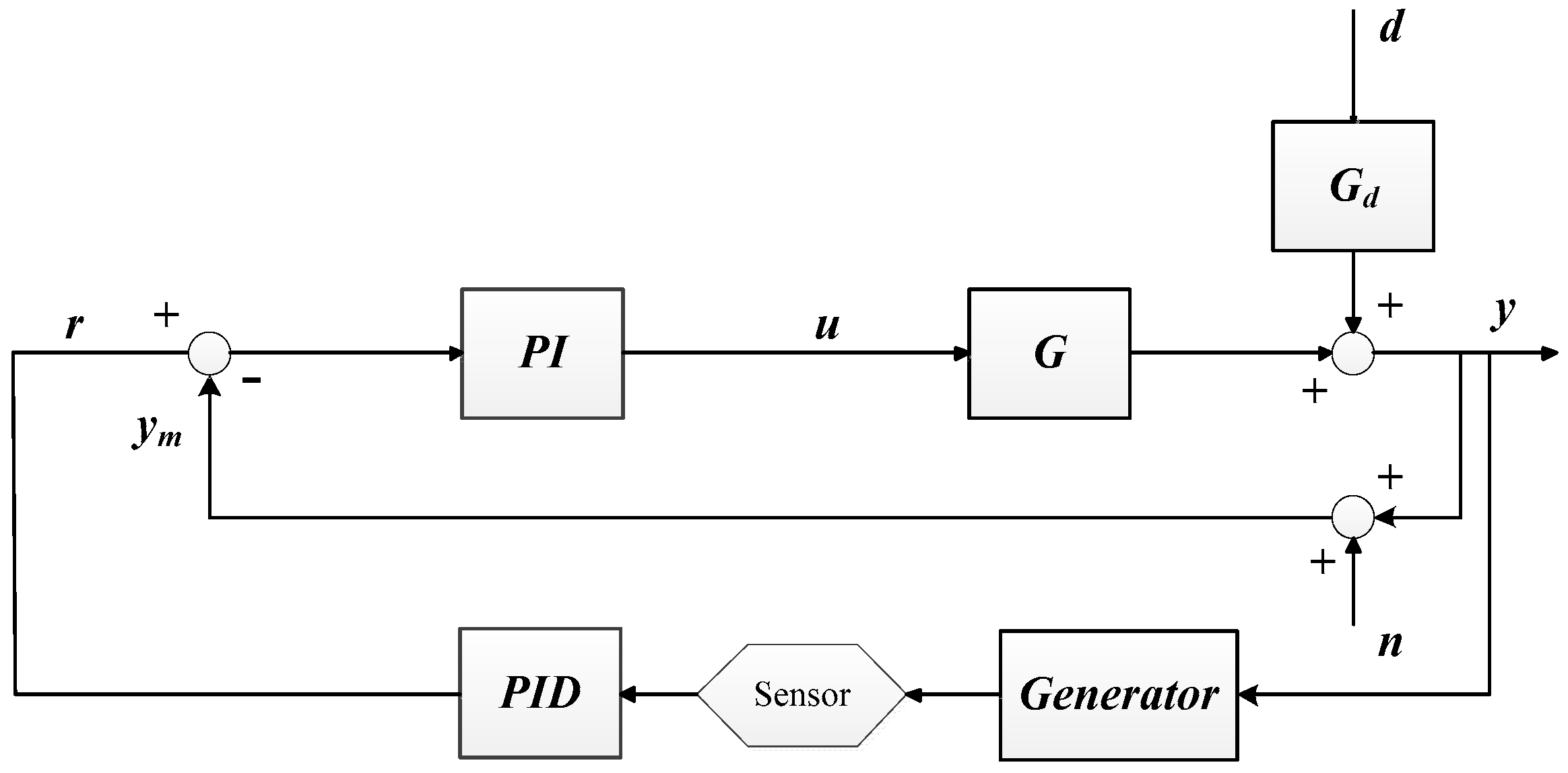
LabVIEW data acquisition control configuration. A: analog; D: digital; NI: national instrument; DAQ: data acquisition; K: core control gain; G: system gain; d: disturbance; Gd: disturbance gain; r: desired process value; ym: measured process variable; u: control variable; n: noisy; y: process variable.
Figure 2.
LabVIEW data acquisition control configuration. A: analog; D: digital; NI: national instrument; DAQ: data acquisition; K: core control gain; G: system gain; d: disturbance; Gd: disturbance gain; r: desired process value; ym: measured process variable; u: control variable; n: noisy; y: process variable.

Figure 3.
Autotuning technique block diagram. e: error; c: controller end; t: relay end; r: desired process value; ym: measured process variable; u: control variable; y: process variable.
Figure 3.
Autotuning technique block diagram. e: error; c: controller end; t: relay end; r: desired process value; ym: measured process variable; u: control variable; y: process variable.

Figure 4.
Overall feedback control flow chart. PID: proportion integration differentiation; NI: national instruments; PI: proportion integration.
Figure 4.
Overall feedback control flow chart. PID: proportion integration differentiation; NI: national instruments; PI: proportion integration.

Figure 5.
Front panel of the hydropower control system virtual instrument (VI).

Figure 6.
Data processing loop of the block diagram.

Figure 7.
Pulse generation loop of the block diagram.

Figure 8.
Autotuning control loop of the block diagram.

Figure 9.
Frequency or voltage maintenance control block diagram.

Figure 10.
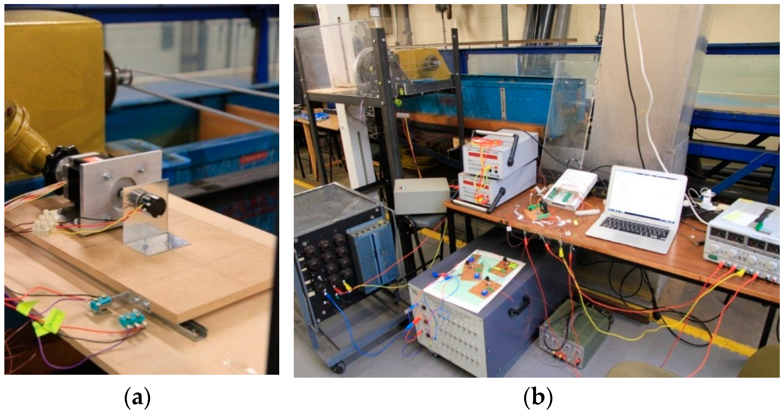
Photograph of the experimental setup for power generator: (a) assembled stepper motor and turbine valve; (b) assembled whole system.
Figure 10.
Photograph of the experimental setup for power generator: (a) assembled stepper motor and turbine valve; (b) assembled whole system.

Figure 11.
A4988 bipolar stepper motor driver: (a) schematic diagram with wiring connections; (b) photograph of the assembly with a cooling fan. VDD: device drive voltage; GND: ground; MS: microstep; DIR: direction; VMOT: motor drive voltage.
Figure 11.
A4988 bipolar stepper motor driver: (a) schematic diagram with wiring connections; (b) photograph of the assembly with a cooling fan. VDD: device drive voltage; GND: ground; MS: microstep; DIR: direction; VMOT: motor drive voltage.

Figure 12.
Potentiometer. (a) Circuit schematic diagram with three ends: ground (GND), voltage source (+5 V) and analog input pin; (b) photograph of the assembly.
Figure 12.
Potentiometer. (a) Circuit schematic diagram with three ends: ground (GND), voltage source (+5 V) and analog input pin; (b) photograph of the assembly.

Figure 13.
Photograph of the experimental setup of the power generator. (a) Circuit schematic diagram; (b) photograph of the assembly.
Figure 13.
Photograph of the experimental setup of the power generator. (a) Circuit schematic diagram; (b) photograph of the assembly.

Figure 14.
NI USB-6221 multifunction data acquisition. (a) Pinouts/front panel connections; (b) photograph of the assembled connections. AI: analog input; AO: analog output; P: port; PFI: front-panel line.
Figure 14.
NI USB-6221 multifunction data acquisition. (a) Pinouts/front panel connections; (b) photograph of the assembled connections. AI: analog input; AO: analog output; P: port; PFI: front-panel line.

Figure 15.
PID relay autotuning.

Figure 16.
Acceptance of the new control gain: (a) Before autotuning; (b) after autotuning.

Figure 17.
Valve position and pulse frequency vs time. (a) Before autotuning; (b) after autotuning.

Figure 18.
Initial state of the graphical user interface of revolutions per minute (RPM) control.

Figure 19.
Graphical user interface of RPM control at 1100 RPM.

Figure 20.
Graphical user interface of RPM control at 1000 RPM.

Figure 21.
Graphical user interface of voltage control at 100 V.

Figure 22.
Graphical user interface of voltage control at 110 V.

Figure 23.
Graphical user interface of voltage control under variable water flow.


Table 1.
NI-USB 6221 performance.
| Control | Voltage Range | Performance | Value |
|---|---|---|---|
| Analog input | 0–10 V | accuracy | 3230 µV |
| Analog output | 0–10 V | drive current | 5 mA |
| Digital input | 0–5 V | max clock rate | 1 MHz |
| Digital output | 0–5 V | drive current | 24 mA |
Table 2.
The Ziegler-Nichols method.
| Control | Performance | P | I | D |
|---|---|---|---|---|
| P | Fast | 0.50 | - | - |
| Normal | 0.20 | - | - | |
| Slow | 0.13 | - | - | |
| PI | Fast | 0.40 | 0.8 | - |
| Normal | 0.18 | 0.8 | - | |
| Slow | 0.13 | 0.8 | - | |
| PID | Fast | 0.60 | 0.5 | 0.12 |
| Normal | 0.25 | 0.5 | 0.12 | |
| Slow | 0.15 | 0.5 | 0.12 |
P: proportional parameter; PI: proportion integration; PID: proportion integration differentiation; I: integration parameter; D: derivative parameter.
Table 3.
A4988 microstep resolution.
| MS1 | MS2 | MS3 | Microstep Resolution | |
|---|---|---|---|---|
| Low | Low | Low | Full Step | 1/1 |
| High | Low | Low | Half Step | 1/2 |
| Low | High | Low | Quarter Step | 1/4 |
| High | High | Low | Eighth Step | 1/8 |
| High | High | High | Sixteenth Step | 1/16 |
© 2018 by the authors. Licensee MDPI, Basel, Switzerland. This article is an open access article distributed under the terms and conditions of the Creative Commons Attribution (CC BY) license (http://creativecommons.org/licenses/by/4.0/).
Share and Cite
MDPI and ACS Style
Fan, Y.; Zhang, D.; Li, J. A Control Scheme for Variable-Speed Micro-Hydropower Plants. Sustainability 2018, 10, 4333. https://doi.org/10.3390/su10114333
AMA Style
Fan Y, Zhang D, Li J. A Control Scheme for Variable-Speed Micro-Hydropower Plants. Sustainability. 2018; 10(11):4333. https://doi.org/10.3390/su10114333
Chicago/Turabian StyleFan, Youping, Dai Zhang, and Jingjiao Li. 2018. "A Control Scheme for Variable-Speed Micro-Hydropower Plants" Sustainability 10, no. 11: 4333. https://doi.org/10.3390/su10114333
Note that from the first issue of 2016, this journal uses article numbers instead of page numbers. See further details here.