Promoting Green and Sustainability: A Multi-Objective Optimization Method for the Job-Shop Scheduling Problem

Abstract

As a result of increasingly serious environmental pollution, it is vital to reduce carbon emissions to achieve green and sustainable development for manufacturing processes. Customer satisfaction, as an important factor affecting enterprise profits, is of great importance in the promotion of sustainable development. Because an accurate delivery time and high delivery rate improve customer satisfaction and enhance an enterprise’s competitive advantage in the market, this paper proposes a new optimization method for achieving low carbon emissions, a high delivery rate, and a low cost for a job-shop scheduling problem. The computational results show the negative correlation between assembly cost and carbon emissions, and the positive correlation between assembly cost and delivery time by Pareto optimization. The proposed method, which takes into consideration carbon emissions, greatly supports the objective of achieving a green and sustainable development.

1. Introduction

Green and sustainable development has become an important aspect of the progression of the manufacturing industry in the future [1,2,3]. As far as the environment is concerned, the “green” highlights the aim of producing the required products with lower carbon emissions so as to reduce the environmental pollution caused by the manufacturing process, and the “sustainable” highlights the aim of producing the required products at a lower cost [4,5]. The enterprises with healthy and sustainable development would have a strong competitiveness advantage in the modern market. As production scheduling plays an important role in the manufacturing process that makes useful of manufacturing resources [6,7,8], it is of great significance for manufacturing enterprises to develop a scheduling method to achieve green and sustainable manufacturing. This paper summarizes the existing research as follows:

(1)

Green and sustainable development aspects: Low carbon is an important indicator of green development, Ding et al. [9] considered a permutation flow-shop scheduling problem with the objectives of minimizing the total carbon emissions and makespan. Liu [10] presented a job-shop scheduling model and established a carbon footprint model to quantify the carbon emission of different scheduling plans, in which three carbon efficiency indicators were put forward to estimate the carbon emission of jobs and equipment. Yin et al. [11] proposed a low-carbon mathematical scheduling model to optimize productivity, energy efficiency, and noise reduction. Liu [12] developed an ε-archived genetic algorithm to examine two-batch scheduling problems to minimize CO₂ emission and total weighted tardiness.

(2)

Optimization objective aspects: Han et al. [13] proposed a multi-objective scheduling model considering the production quality, the makespan, and equipment performance. Gong et al. [14] introduced a multi-objective model for intelligent production systems to schedule jobs, equipment idleness, and human resource under real-time electricity pricing. Besides, many research usually simplify the complex processing environment into a single equipment production problem to facilitate the calculation [15,16,17]. Li et al. [18] studied a single equipment scheduling problem to determine the maintenance activity and job sequence. González et al. [19] tackled a single equipment scheduling problem with sequence-dependent setup time to minimize the weighted tardiness.

(3)

Equipment maintenance aspects: Preventive maintenance plays an important role in continuous production. Feng et al. [20] integrated imperfect preventive maintenance and sequence-dependent group scheduling in flow-shop manufacturing cells, and proposed a system-level model. Tayeb et al. [21] introduced a game theory approach for a permutation flow-shop scheduling problem to meet production and maintenance criteria. Gholami et al. [22] presented the hybrid flow-shop and scheduling overview of the equipment in the case of random availability, and integrated the simulation into the genetic algorithm for the random fault equipment scheduling mixed-model shop. Wong et al. [23] developed a real-time segmented rescheduling method for dynamic factors and used a genetic algorithm for the pre-stitching process of dynamic garment manufacturing.

Through the abovementioned literature, it can be found that in solving the green and sustainable scheduling problem, existing contributions focus on how to transform multi-objective optimization into single-objective optimization [24,25,26], ignoring the balance of multi-objectives. In addition, these consider the delivery time window [27] without using it as a constraint. Much of the literature focuses on applying carbon emissions for power dispatching problems, but not for scheduling problems in the manufacturing process [28]. Despite this, there is extensive literature focused on equipment maintenance and multi-objective optimization [29,30], however how to solve the scheduling problems of low-carbon and sustainable development has become a research gap, especially taking delivery time as one objective for customer satisfaction so as to promote the circular sustainable development of enterprises. The aim of this study is to fill this research gap and provide guidance for the government and firms whose focus is achieving green and sustainability development.

Our proposal is motivated by the importance of providing a new multi-objective optimization method for the job-shop scheduling problem to promote green and sustainable development in the manufacturing industry. This study assumes that equipment faults obey the Weibull distribution, and aims to provide an improved genetic algorithm to solve the multi-objective workshop scheduling model. This model and method will also provide a guidance for enterprises to analyze the key factors affecting carbon emissions and costs, and formulate targeted countermeasures to achieve green and sustainable development. In addition, this study hopes to provide reference value for scholars engaged in the research of green production scheduling. Furthermore, this paper develops a new method to minimize carbon emissions and cost, and maximize the product delivery. Accordingly, three methods are used to solve this problem: an improved genetic algorithm (I-GA), a genetic algorithm (GA), and a clonal immune algorithm (CIA). In addition, the relationship between assembly cost and carbon emissions in the production process is discussed.

2. Problem Description

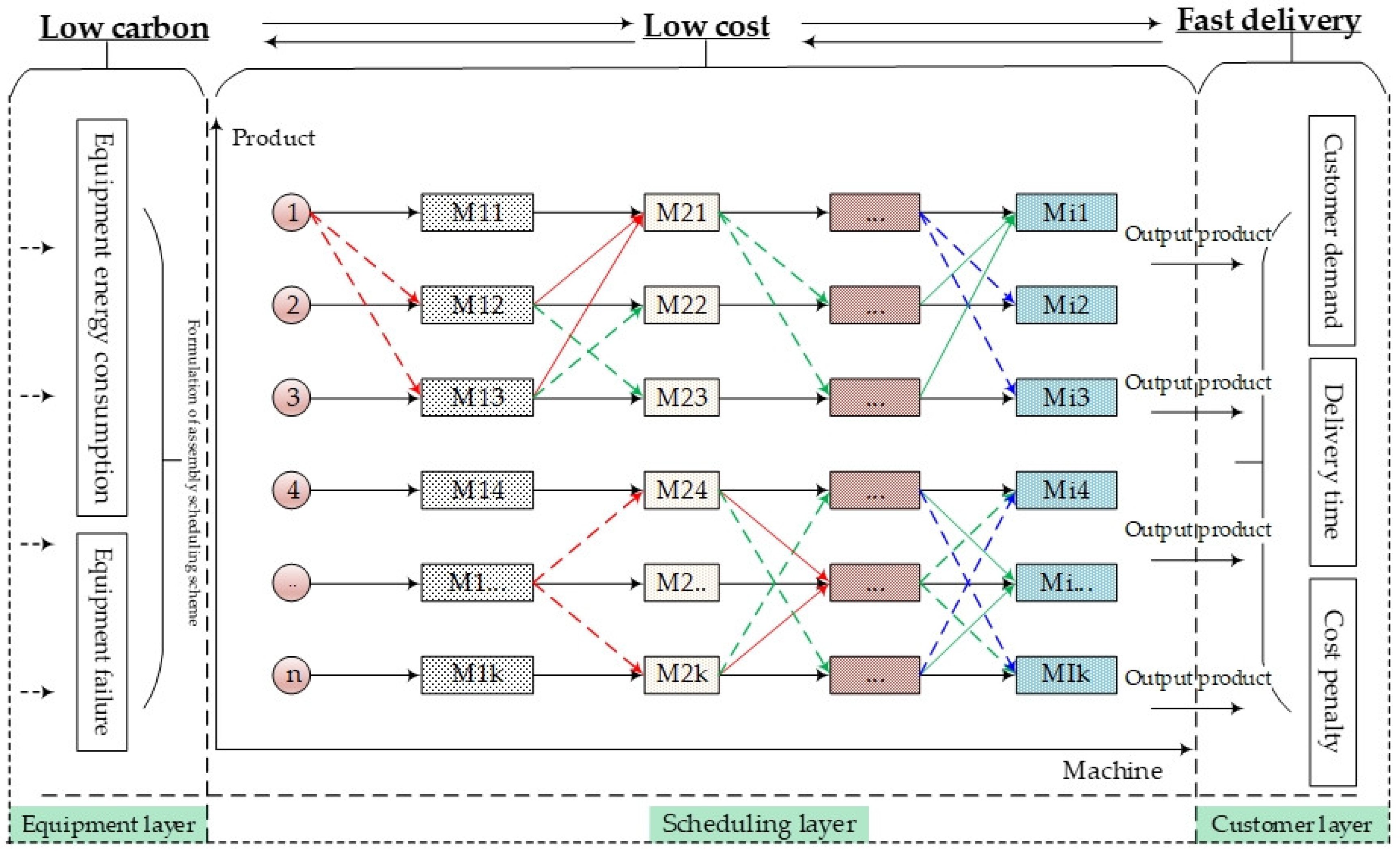
There are $N$ work pieces to be processed in S stages on an assembly line. The work pieces pass through the stages in turn and each stage consists of $K$ pieces of equipment. There is at least one piece of equipment in each stage. Each work piece has to undergo an assembly process at each stage. There are three maintenance strategies for equipment failure, including minor repair, major repair, and replacement. The maintenance operations are required as much as possible during the idle state of the equipment. The basic assembly model is shown in Figure 1.

Figure 1. represents the basic assembly model, where Mik represents the number of machine. Assume all work pieces arrive at time zero, and preventive maintenance cannot interrupt the processing. The parameters and decision variables are shown in

Table 1. The parameters and decision variables.

$t_{[\mathrm{i}][\mathrm{j}][\mathrm{k}]}^{pm}$ time of minor maintenance	$R_0$ equipment’s initial reliability
$t_{[\mathrm{i}][\mathrm{j}][\mathrm{k}]}^{po}$ time of overhaul maintenance	${\omega }_{[\mathrm{k}]}$ the value waste of equipment caused by the replacement
$t_{[\mathrm{i}][\mathrm{j}][\mathrm{k}]}^{pr}$ time of replacement during maintenance	$R({\mathrm{a}}_{[\mathrm{k}-1]})$ reliability of equipment k before replacement operation
$t_{[\mathrm{i}][\mathrm{j}][\mathrm{k}]}^{mr}$ the repair time	${\nu }_{[\mathrm{k}]}$ utilization value of equipment k from initial state to complete deterioration
$t_{setup}$ setup time of the equipment	$d^m$ the earliest time of the customer’s demand
$\vartheta$ the acceleration penalty factor	$d^n$ the latest time of the customer’s demand
$\partial$ the operation cost per unit time	$L_{md}$ unit time loss cost of equipment during preventive maintenance downtime
$c_{[\mathrm{i}][\mathrm{j}][\mathrm{k}]}^{pm}$ cost of minor maintenance	$L_{bd}$ unit time loss cost of the equipment during breakdown downtime
$c_{[\mathrm{i}][\mathrm{j}][\mathrm{k}]}^{po}$ cost of overhaul maintenance	$Z_{[\mathrm{i}][\mathrm{j}][\mathrm{k}]}^1$ the power consumption of equipment k in standby state
$c_{[\mathrm{i}][\mathrm{j}][\mathrm{k}]}^{pr}$ cost of replacement during maintenance	$Z_{[\mathrm{i}][\mathrm{j}][\mathrm{k}]}^3$ the power consumption of equipment k during processing
$c_{[\mathrm{i}][\mathrm{j}][\mathrm{k}]}^{mr}$ the cost of repair	$Z_{[\mathrm{i}][\mathrm{j}][\mathrm{k}]}^4$ the power consumption of equipment k during no-load operating
$C_{[\mathrm{i}][\mathrm{j}][\mathrm{k}]}^{mr}$ total cost of repair	$T_{[\mathrm{i}][\mathrm{j}][\mathrm{k}]}^2$ time required for the equipment from the startup state to the steady state
$C_{[\mathrm{i}][\mathrm{j}][\mathrm{k}]}^p$ total cost of maintenance	$T_{[\mathrm{i}][\mathrm{j}][\mathrm{k}]}^{2^{\prime }}$ time required for equipment from clicking shutdown to stable stop state
$C_{pe}$ the penalty cost	$T_{[\mathrm{i}][\mathrm{j}][\mathrm{k}]}^1$ time of equipment k in standby state
$C_{[\mathrm{i}][\mathrm{j}][\mathrm{k}]}^f$ fixed costs	$T_{[\mathrm{i}][\mathrm{j}][\mathrm{k}]}^3$ time of equipment k during processing
$\rho$ carbon emissions per unit of energy consumption	$T_{[\mathrm{i}][\mathrm{j}][\mathrm{k}]}^4$ no-load operating time of equipment k
$Q$ total energy consumption	$t_{[i][j][k]}$ the processing time of the j process of the i product on the equipment k
$Q_{\mathrm{carbon}}$ the amount of carbon dioxide emissions	$a$ start time point of equipment
$b$ stop running time point of equipment	$P_k(\mathrm{t})$ input power of equipment k at time t

.

3. Multi-Objective Optimization Method

3.1. Cost Analysis for Assembly Operation

As a result of the preventive maintenance of the equipment, the equipment will be shut down, which will bring economic losses to the enterprise. Therefore, time value, actual maintenance cost, and value waste are taken into account when calculating the equipment preventive maintenance cost in this paper. The maintenance cost respectively is

$$C_{\left[i\right]\left[j\right]\left[k\right]}^{pm}=L_{md}{t}_{\left[i\right]\left[j\right]\left[k\right]}^{pm}+c_{\left[i\right]\left[j\right]\left[k\right]}^{pm}$$

(1)

$$C_{\left[i\right]\left[j\right]\left[k\right]}^{po}=L_{md}{t}_{\left[i\right]\left[j\right]\left[k\right]}^{po}+c_{\left[i\right]\left[j\right]\left[k\right]}^{po}$$

(2)

$$C_{\left[i\right]\left[j\right]\left[k\right]}^{pr}=L_{md}{t}_{\left[i\right]\left[j\right]\left[k\right]}^{pr}+c_{\left[i\right]\left[j\right]\left[k\right]}^{pr}$$

(3)

The repair cost is calculated:

$$C_{\left[i\right]\left[j\right]\left[k\right]}^{mr}=L_{bd}{t}_{\left[i\right]\left[j\right]\left[k\right]}^{mr}+c_{\left[i\right]\left[j\right]\left[k\right]}^{mr}$$

(4)

Based on Equations (1)–(4), it can be obtained that

$$\begin{gathered} C_1={{\displaystyle \sum }}_{i\in I}{{\displaystyle \sum }}_{j\in I}{{\displaystyle \sum }}_{k\in K}{C}_{\left[i\right]\left[j\right]\left[k\right]}^{pm}+{{\displaystyle \sum }}_{i\in I}{{\displaystyle \sum }}_{j\in I}{{\displaystyle \sum }}_{k\in K}{C}_{\left[i\right]\left[j\right]\left[k\right]}^{po}+{{\displaystyle \sum }}_{i\in I}{{\displaystyle \sum }}_{j\in I}{{\displaystyle \sum }}_{k\in K}{C}_{\left[i\right]\left[j\right]\left[k\right]}^{pr}+ \\ {{\displaystyle \sum }}_{i\in I}{{\displaystyle \sum }}_{j\in I}{{\displaystyle \sum }}_{k\in K}{C}_{\left[i\right]\left[j\right]\left[k\right]}^{mr} \end{gathered}$$

(5)

The value waste of equipment will be calculated according to the reliability. That is

$${\omega }_{\left[k\right]}=\frac{R\left(a_{\left[k-1\right]}\right)}{R_0}$$

(6)

The replacement of equipment will lead to the salvage value waste of equipment, and the value waste will bring additional cost to the enterprise. The value waste of different equipment is related to the equipment type. Therefore, a constant related to the equipment type is introduced. The cost of value waste caused by equipment replacement can be calculated as

$$C_2={\nu }_{\left[k\right]}\times {\omega }_{\left[k\right]}$$

(7)

In addition, customer’s demand can be represented by the time window $\left[d^m,d^n\right]$. When the completion time falls into the time window, the assembly task is completed according to the customer’s requirements. When the completion time deviates from the time window, it means that the customer’s demand cannot be met. The penalty diagram of the time window constraint is shown in Figure 2 ($d^1$, $d^2$, $d^3$, $d^4$ represents penalty threshold of time windows).

Different lengths of the assembling operation may lead to the advance or extension of the delivery time, which may lead to customer dissatisfaction and loss of profit. In order to avoid the penalty cost and promote enterprise’s sustainable development, a penalty cost function is given as

$$C_{pe}=\{\begin{array}{ll}\frac{d^m-t^{\prime }}{d^n-d^m}\times \vartheta ,& t^{\prime }\in [{\mathrm{d}}^1,d^2)\\ \frac{d^m-t^{\prime }}{d^n-d^m},& t^{\prime }\in [{\mathrm{d}}^2,d^m)\\ 0,& t^{\prime }\in [{\mathrm{d}}^m,{\mathrm{d}}^n]\\ \frac{t^{\prime }-d^m}{d^n-d^m},& t^{\prime }\in [{\mathrm{d}}^n,d^3)\\ \frac{d^m-t^{\prime }}{d^n-d^m}\times \vartheta ,& t^{\prime }\in [{\mathrm{d}}^3,d^4)\end{array}$$

(8)

where $d^1$, $d^2$, $d^3$, $d^4$ are constant. In Equation (8), the penalty cost can be used to express the customer’s unsatisfied rate of delivery time. The larger the penalty value is, the larger the customer’s unsatisfied rate is. As a result of the operation cost related to normal working time, the operation costs $C_o$ can be given as

$$C_o=\partial {{\displaystyle \sum }}_{i\in I}{{\displaystyle \sum }}_{j\in I}{{\displaystyle \sum }}_{k\in K}{t}_{\left[i\right]\left[j\right]\left[k\right]}$$

(9)

As the fixed cost $C_{\left[i\right]\left[j\right]\left[k\right]}^f$ is incurred by each equipment start-up including labor cost and depreciation cost. So the total assembly costs including preventive maintenance costs, repair costs, costs of value waste caused by replacements, penalty costs, operational costs, and fixed costs can be expressed as

$$\begin{gathered} C={{\displaystyle \sum }}_{i\in I}{{\displaystyle \sum }}_{j\in I}{{\displaystyle \sum }}_{k\in K}{C}_{\left[i\right]\left[j\right]\left[k\right]}^{pm}+{{\displaystyle \sum }}_{i\in I}{{\displaystyle \sum }}_{j\in I}{{\displaystyle \sum }}_{k\in K}{C}_{\left[i\right]\left[j\right]\left[k\right]}^{po}+{{\displaystyle \sum }}_{i\in I}{{\displaystyle \sum }}_{j\in I}{{\displaystyle \sum }}_{k\in K}{C}_{\left[i\right]\left[j\right]\left[k\right]}^{pr}+ \\ {{\displaystyle \sum }}_{i\in I}{{\displaystyle \sum }}_{j\in I}{{\displaystyle \sum }}_{k\in K}{C}_{\left[i\right]\left[j\right]\left[k\right]}^{mr}+ {\nu }_{\left[k\right]}\times {\omega }_{\left[k\right]}+C_{pe}+\partial {{\displaystyle \sum }}_{i\in I}{{\displaystyle \sum }}_{j\in I}{{\displaystyle \sum }}_{k\in K}{t}_{\left[i\right]\left[j\right]\left[k\right]}+ \\ {{\displaystyle \sum }}_{i\in I}{{\displaystyle \sum }}_{j\in I}{{\displaystyle \sum }}_{k\in K}{C}_{\left[i\right]\left[j\right]\left[k\right]}^f \end{gathered}$$

(10)

3.2. Carbon Analysis for Assembly Operation

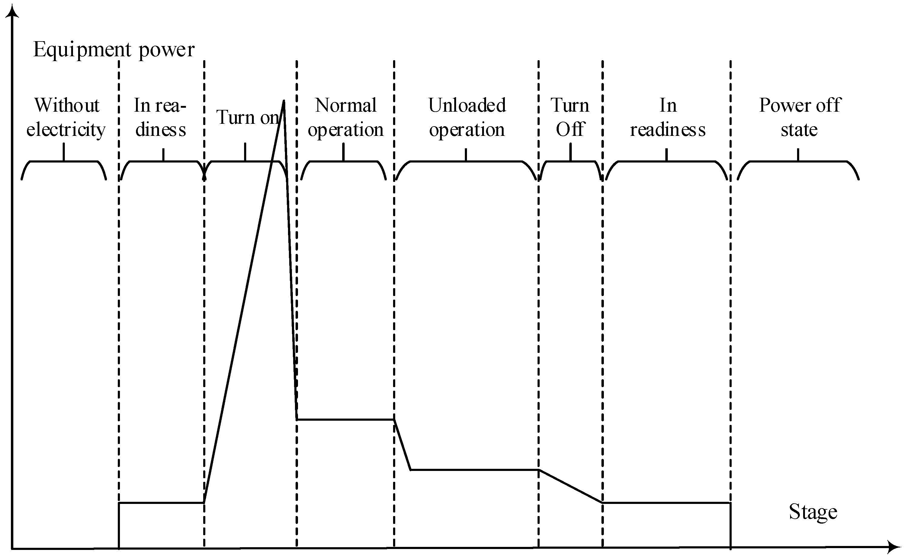
Under normal circumstances, equipment with different gears can be divided into the power-off phase, the standby phase, the equipment start-up phase, the low-speed operation phase, the no-load operation phase, the mid-range operation phase, the high-speed operation phase, and the equipment shutdown phase. The equipment power under different stages is shown in Figure 3.

In order to obtain the energy consumption in the assembly process, the equipment’s operation is divided into different stages: standby energy consumption, on/off energy consumption, energy consumption in production, and energy consumption of no-load equipment.

(1) Standby energy consumption

When the equipment is in the standby phase, the power consumption will be caused by the equipment activating. Suppose the energy consumption in the standby phase is represented by $Q_1$. There is

$$Q_1={{\displaystyle \sum }}_{i\in I}{{\displaystyle \sum }}_{j\in I}{{\displaystyle \sum }}_{k\in K}{z}_{\left[i\right]\left[j\right]\left[k\right]}^1{T}_{\left[i\right]\left[j\right]\left[k\right]}^1$$

(11)

(2) On/off energy consumption

It takes a period of time from the start-up of the equipment to stable operation, and from the shutdown of the equipment to the stop operation state. Although the product assembly operation cannot be carried out during this period, certain energy consumption will be caused. The energy consumption can be expressed by equipment power and its running time, shown as

$$Q_2={{\displaystyle \int }}_a^{a+T_{\left[i\right]\left[j\right]\left[k\right]}^2}{P}_k\left(t\right)dt+{{\displaystyle \int }}_{b-T_{\left[i\right]\left[j\right]\left[k\right]}^2}^b{P}_k\left(t\right)dt$$

(12)

(3) Energy consumption in production

While the equipment is in production, a large amount of energy will be consumed. The energy consumption is

$$Q_3={{\displaystyle \sum }}_{i\in I}{{\displaystyle \sum }}_{j\in I}{{\displaystyle \sum }}_{k\in K}{z}_{\left[i\right]\left[j\right]\left[k\right]}^3{T}_{\left[i\right]\left[j\right]\left[k\right]}^3$$

(13)

(4) Energy consumption of no-load equipment

Between the completion of the previous assembly process and the start of the next assembly process, the equipment status is shown in two ways: one is to continue the no-load operation, the other is to shut down to stop the operation state, until the next process restarts the equipment. The energy consumption of the no-load state of the equipment is expressed quantitatively, indicating the energy consumption of the no-load operation of the equipment, shown as follow:

According to the above four formulas, the total energy consumption of the equipment in the process of assembly can be obtained. The carbon emission calculation method during the whole assembly process can be obtained according to the energy consumption of the equipment. Therefore, the calculation formula of the carbon emission during the assembly process is presented as

$$\begin{gathered} Q_{carbon}=\rho ({{\displaystyle \sum }}_{i\in I}{{\displaystyle \sum }}_{j\in I}{{\displaystyle \sum }}_{k\in K}{z}_{\left[i\right]\left[j\right]\left[k\right]}^1{T}_{\left[i\right]\left[j\right]\left[k\right]}^1+{{\displaystyle \int }}_a^{a+T_{\left[i\right]\left[j\right]\left[k\right]}^2}{P}_k\left(t\right)dt+{{\displaystyle \int }}_{b-T_{\left[i\right]\left[j\right]\left[k\right]}^2}^b{P}_k\left(t\right)dt+ \\ {{\displaystyle \sum }}_{i\in I}{{\displaystyle \sum }}_{j\in I}{{\displaystyle \sum }}_{k\in K}{z}_{\left[i\right]\left[j\right]\left[k\right]}^3{T}_{\left[i\right]\left[j\right]\left[k\right]}^3+{{\displaystyle \sum }}_{i\in I}{{\displaystyle \sum }}_{j\in I}{{\displaystyle \sum }}_{k\in K}{z}_{\left[i\right]\left[j\right]\left[k\right]}^4{T}_{\left[i\right]\left[j\right]\left[k\right]}^4) \end{gathered}$$

(14)

3.3. Delivery Time Analysis of Assembly Operation

Assume that the failure rate of the assembly equipment follows the Weibull distribution with the shape parameter $\beta$ and the size parameter $\eta$. Thus, the equipment failure rate function $\lambda \left(t\right)$ is shown as

$$\lambda \left(t\right)=\frac{\beta }{\eta }{\left(\frac{t}{\eta }\right)}^{\beta -1}{e}^{-{\left(\raisebox{1ex}{$t$}\!\left/ \!\raisebox{-1ex}{$\eta $}\right.\right)}^{\beta }}$$

(15)

According to the equipment failure rate function, the expected number of equipment failures in the maintenance period $\tau$ can be deduced, and $m\left(\tau \right)$ is used to represent the expected number of failures during the maintenance period $\tau$. $m\left(\tau \right)$ is calculated as

$$m\left(\tau \right)={{\displaystyle \int }}_0^{\tau }\lambda \left(t\right)dt={{\displaystyle \int }}_0^{\tau }\frac{\beta }{\eta }{\left(\frac{t}{\eta }\right)}^{\beta -1}{e}^{-{\left(\raisebox{1ex}{$t$}\!\left/ \!\raisebox{-1ex}{$\eta $}\right.\right)}^{\beta }}dt$$

(16)

Among them, the probability density function and probability distribution function of equipment failure obeying the Weibull distribution are shown in Figure 4. According to the basic properties of the Weibull function, the frequency of equipment in a fixed period can be deduced.

According to Figure 4 and Equation (16), the expected failure time of the equipment can be obtained. That is

$$T_1={\displaystyle \sum }{t}_{\left[i\right]\left[j\right]\left[k\right]}^{\left[\right]}{{\displaystyle \int }}_0^{\tau }\frac{\beta }{\eta }{\left(\frac{t}{\eta }\right)}^{\beta -1}{e}^{-{\left(\raisebox{1ex}{$t$}\!\left/ \!\raisebox{-1ex}{$\eta $}\right.\right)}^{\beta }}dt$$

(17)

where $t_{\left[i\right]\left[j\right]\left[k\right]}^{\left[\right]}$ represents the time required for different maintenance strategies, which include minor repair, overhaul, and replacement (i.e., $t_{\left[i\right]\left[j\right]\left[k\right]}^{pm}$, $t_{\left[i\right]\left[j\right]\left[k\right]}^{po}$, $t_{\left[i\right]\left[j\right]\left[k\right]}^{pr}$).

Theorem 1.

Suppose$y_{\left[i\right]\left[j\right]\left[k\right]}$is used to indicate the maintenance strategy, and the strategy for minor repair, overhaul, and replacement is expressed by 1, 2, and 3, respectively. The maintenance time of equipment failure, that is, the calculation formula for the equipment shutdown time, can be deduced as follows:

$$t_{[\mathrm{i}][\mathrm{j}][\mathrm{k}]}^{[]}=\frac{1}{2}\left\{(3-y_{[\mathrm{i}][\mathrm{j}][\mathrm{k}]})(2-y_{[\mathrm{i}][\mathrm{j}][\mathrm{k}]})t_{[\mathrm{i}][\mathrm{j}][\mathrm{k}]}^{pm}+\left[(t_{[\mathrm{i}][\mathrm{j}][\mathrm{k}]}^{pr}+t_{[\mathrm{i}][\mathrm{j}][\mathrm{k}]}^{po})+(2y_{[\mathrm{i}][\mathrm{j}][\mathrm{k}]}-5)(t_{[\mathrm{i}][\mathrm{j}][\mathrm{k}]}^{pr}-t_{[\mathrm{i}][\mathrm{j}][\mathrm{k}]}^{po})\right](2.5y_{[\mathrm{i}][\mathrm{j}][\mathrm{k}]}-0.5y_{[\mathrm{i}][\mathrm{j}][\mathrm{k}]}{y}_{[\mathrm{i}][\mathrm{j}][\mathrm{k}]}-2)\right\}$$

(18)

In Equation (18), there is

$$y_{[i][j][k]}=\{\begin{array}{l}1,\mathrm{minor}\mathrm{repairs}\mathrm{before}\mathrm{the}\mathrm{operation}\mathrm{of}\mathrm{the}\mathrm{assembly}\mathrm{process}\\ 2,\mathrm{overhaul}\mathrm{before}\mathrm{the}\mathrm{operation}\mathrm{of}\mathrm{the}\mathrm{assembly}\mathrm{process}\\ 3,\mathrm{replacement}\mathrm{before}\mathrm{the}\mathrm{operation}\mathrm{of}\mathrm{the}\mathrm{assembly}\mathrm{process}\end{array}$$

(19)

where $k=1,2,\dots ,K$.

Proof. 

(a) While using a minor repair strategy (i.e., $y_{\left[i\right]\left[j\right]\left[k\right]}=1$), substituting $y_{\left[i\right]\left[j\right]\left[k\right]}=1$ into Equation (18) results in the following Equation (20).

$$t_{[\mathrm{i}][\mathrm{j}][\mathrm{k}]}^{[]}=\frac{1}{2}\left\{(3-1)(2-1)t_{[\mathrm{i}][\mathrm{j}][\mathrm{k}]}^{pm}+\left[(t_{[\mathrm{i}][\mathrm{j}][\mathrm{k}]}^{pr}+t_{[\mathrm{i}][\mathrm{j}][\mathrm{k}]}^{po})+(2-5)(t_{[\mathrm{i}][\mathrm{j}][\mathrm{k}]}^{pr}-t_{[\mathrm{i}][\mathrm{j}][\mathrm{k}]}^{po})\right](2.5-0.5-2)\right\}=t_{[\mathrm{i}][\mathrm{j}][\mathrm{k}]}^{pm}$$

(20)

It means that while a minor repair strategy is adopted, the equipment maintenance time is $t_{\left[i\right]\left[j\right]\left[k\right]}^{pm}$.

(b) While using an overhaul maintenance strategy (i.e., $y_{\left[i\right]\left[j\right]\left[k\right]}=2$), substituting $y_{\left[i\right]\left[j\right]\left[k\right]}=2$ into Equation (18) results in the following Equation (21).

$$t_{[\mathrm{i}][\mathrm{j}][\mathrm{k}]}^{[]}=\frac{1}{2}\left\{(3-2)(2-2)t_{[\mathrm{i}][\mathrm{j}][\mathrm{k}]}^{pm}+\left[(t_{[\mathrm{i}][\mathrm{j}][\mathrm{k}]}^{pr}+t_{[\mathrm{i}][\mathrm{j}][\mathrm{k}]}^{po})+(4-5)(t_{[\mathrm{i}][\mathrm{j}][\mathrm{k}]}^{pr}-t_{[\mathrm{i}][\mathrm{j}][\mathrm{k}]}^{po})\right](5-2-2)\right\}=t_{[\mathrm{i}][\mathrm{j}][\mathrm{k}]}^{po}$$

(21)

It means that while an overhaul maintenance strategy is adopted, the equipment maintenance time is $t_{\left[i\right]\left[j\right]\left[k\right]}^{po}$, which is consistent with the assumption.

(c) While using a replacement maintenance strategy (i.e.,$y_{\left[i\right]\left[j\right]\left[k\right]}=3$), substituting $y_{\left[i\right]\left[j\right]\left[k\right]}=3$ into Equation (18) results in the following Equation (22).

$$t_{[\mathrm{i}][\mathrm{j}][\mathrm{k}]}^{[]}=\frac{1}{2}\left\{(3-3)(2-3)t_{[\mathrm{i}][\mathrm{j}][\mathrm{k}]}^{pm}+\left[(t_{[\mathrm{i}][\mathrm{j}][\mathrm{k}]}^{pr}+t_{[\mathrm{i}][\mathrm{j}][\mathrm{k}]}^{po})+(6-5)(t_{[\mathrm{i}][\mathrm{j}][\mathrm{k}]}^{pr}-t_{[\mathrm{i}][\mathrm{j}][\mathrm{k}]}^{po})\right](9\ast 2.5-3\ast 0.5-2)\right\}=t_{[\mathrm{i}][\mathrm{j}][\mathrm{k}]}^{pr}$$

(22)

It means that while a replacement maintenance strategy is adopted, the equipment maintenance time is $t_{\left[i\right]\left[j\right]\left[k\right]}^{pr}$, which is consistent with the assumption. □

Thus, it can be obtained that the time of the fault response mechanism $T_2$ is

$$T_2={\displaystyle \sum }{t}_{setup}$$

(23)

Assuming now that $T_3$ represents the processing time of the $j$ process of the $i$ product on the equipment $k$, and the processing time is

$$T_3={{\displaystyle \sum }}_{i\in I}{{\displaystyle \sum }}_{j\in I}{{\displaystyle \sum }}_{k\in K}{t}_{\left[i\right]\left[j\right]\left[k\right]}$$

(24)

3.4. Improved Genetic Algorithm

This paper comprehensively considers preventive maintenance and the penalty cost which increases with the delivery time window as constraints. With the objectives of minimizing the total assembly costs, minimizing the amount of assembly carbon emission, and the assembly completion time, the optimization model is shown in the following Equations (25)–(27).

$$\begin{array}{l}\min C={\displaystyle \sum _{i\in I}}{\displaystyle \sum _{j\in I}}{\displaystyle \sum _{k\in K}}{C}_{\left[i\right]\left[j\right]\left[k\right]}^{pm}+{\displaystyle \sum _{i\in I}}{\displaystyle \sum _{j\in I}}{\displaystyle \sum _{k\in K}}{C}_{\left[i\right]\left[j\right]\left[k\right]}^{po}+{\displaystyle \sum _{i\in I}}{\displaystyle \sum _{j\in I}}{\displaystyle \sum _{k\in K}}{C}_{\left[i\right]\left[j\right]\left[k\right]}^{pr}\\ +{\displaystyle \sum _{i\in I}}{\displaystyle \sum _{j\in I}}{\displaystyle \sum _{k\in K}}{C}_{\left[i\right]\left[j\right]\left[k\right]}^{mr}+{\nu }_{\left[k\right]}\times {\omega }_{\left[k\right]}+C_{pe}+\partial {\displaystyle \sum _{i\in I}}{\displaystyle \sum _{j\in I}}{\displaystyle \sum _{k\in K}}{t}_{\left[i\right]\left[j\right]\left[k\right]}\\ +{\displaystyle \sum _{i\in I}}{\displaystyle \sum _{j\in I}}{\displaystyle \sum _{k\in K}}{C}_{\left[i\right]\left[j\right]\left[k\right]}^f\end{array}$$

(25)

$$\min Q_{carbon}=\rho \times {\displaystyle \sum }\left(Q_1+Q_2+Q_3+Q_4\right)$$

(26)

$$\min T={\displaystyle \sum }\left(T_1+T_2+T_3\right)$$

(27)

where $C$ represents the cost of the assembly operation, $Q_{carbon}$ represents the amount of carbon emissions during the assembly process, and $T$ represents the completion time of the assembly operation. The details are shown hereafter: total assembly costs include preventive maintenance costs, repair costs, costs of value waste caused by replacement, penalty costs, operation costs, and fixed costs. The amount of assembly carbon emission include different amounts under the four different states, respectively. The assembly completion time consists of equipment maintenance time, fault response mechanism time (setup time), and processing time.

In this paper, a genetic algorithm (GA) is improved, the efficiency coefficient method is used to transform the multiple current problem into a single goal. A detailed description is given below.

(1.) Multiple objective transformation

In the production scheduling process under the Flexible Job-shop Scheduling Problem (FJSP) mode, the “efficiency coefficient method” was adopted to convert the three goals of minimizing assembly cost $C$, minimizing amounts of carbon emission $Q,$ and minimizing completion time $T$ into a single goal. The conversion is

$$f_1=\sqrt{e^{-e\left(\frac{C-a_1}{a_0-a_1}\right)}{e}^{-e\left(\frac{Q-b_1}{b_0-b_1}\right)}{e}^{-e\left(\frac{T-c_1}{c_0-c_1}\right)}}$$

(28)

where $a_0$, $b_0$, and $c_0$ represent the unqualified threshold of minimizing the assembly cost, minimizing carbon emissions, and minimizing the completion time, respectively. $a_1$, $b_1$, and $c_1$ represent the qualified threshold of minimizing the assembly cost, minimizing carbon emissions, and minimizing the completion time, respectively. Their values are determined according to the historical data of production scheduling.

(2.) Chromosome coding

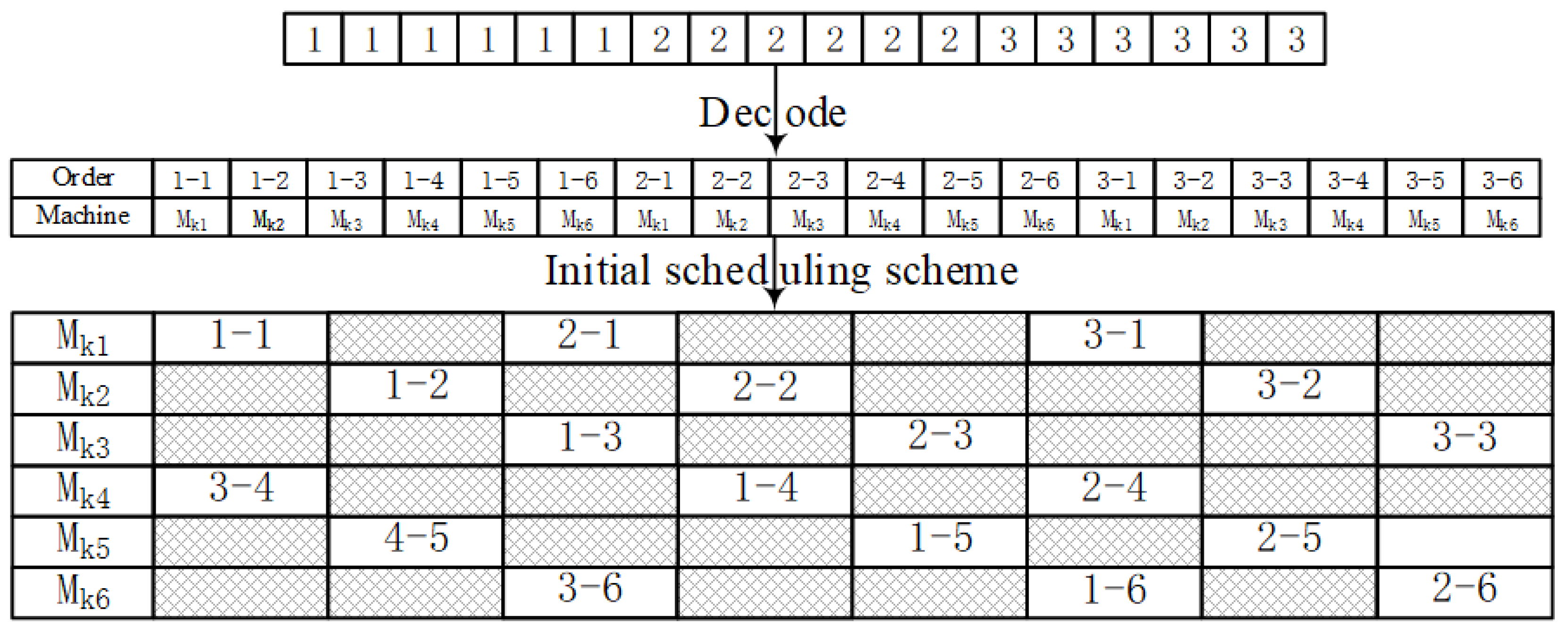
The two-layer coding is carried out in the form of a real number system. The encoding and decoding of chromosomes are shown in Figure 5 during production scheduling.

According to Figure 5, the first layer is the product process coding. When the number first appears, it is expressed as the first process of the product, such as 1, 1, 1, 2, 2, 2, and so on. In turn, it represents the first processes, second processes, and third processes of product No. 1, etc. until the third processes of product No. 2. The second layer is equipment coding, indicating the equipment corresponding to the product process. According to the two-layer coding rules, the processing sequence of products and the corresponding equipment can be decoded.

(3.) Fitness function

Fitness function plays an important role in the evolution of the genetic algorithm to determine whether the chromosome should carry out the next evolutionary operation. In the design of the fitness function, this paper converts multiple goals into a single goal including function with efficiency coefficient, and takes the new single goal inverse as the fitness function, indicating that the closer the optimization goal is, the higher the fitness value of the population will be. According to the mutation probability function, the highly adaptable chromosome is retained in proportion, and it is also evolutionarily manipulated to converge to the optimal goal value faster. The fitness function is shown as

$$f_2=\frac{1}{\sqrt{e^{-e\left(\frac{C-a_1}{a_0-a_1}\right)}{e}^{-e\left(\frac{Q-b_1}{b_0-b_1}\right)}{e}^{-e\left(\frac{T-c_1}{c_0-c_1}\right)}}}$$

(29)

(4.) Crossover operator

In the initial population, according to the crossover probability, a number of chromosomes are randomly selected for the crossover operation. The crossover probability formula is given as

$$p_c=\{\begin{array}{cc}{p}_{c1}-\frac{\left(p_{c1}-p_{c2}\right)\left(f^{\prime }-f_{avg}\right)}{f_{max}-f_{avg}},& f^{\prime }\ge f_{avg}\\ p_{c1},& f^{\prime }<f_{avg}\end{array}$$

(30)

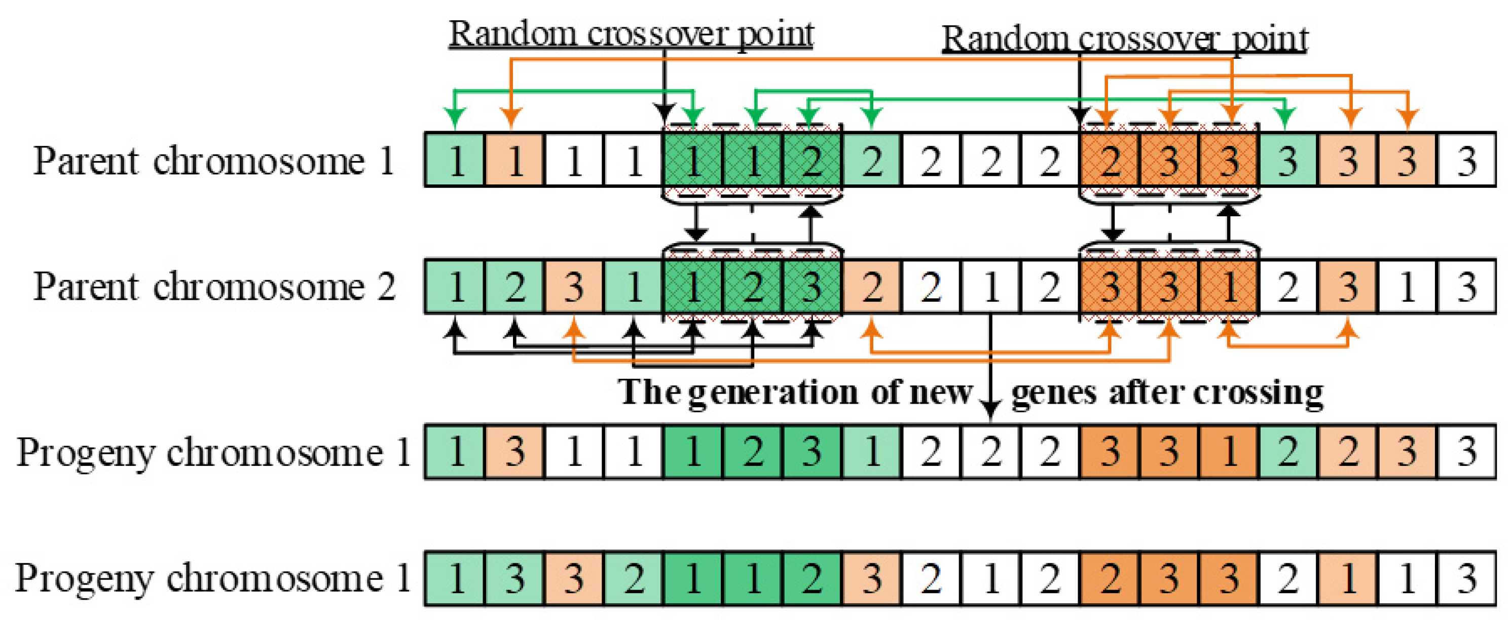
In Equation (30), $p_{c1}$ and $p_{c2}$ are random variables within $\left(0,1\right)$ to control the cross population. $f^{\prime }$ represents the individual fitness value of the current population, $f_{max}$ represents the maximum fitness value of the individual function in the current population, and $f_{avg}$ represents the average fitness value of the individual in the current population. According to the crossover probability, chromosome crossover was determined. In this paper, a two-point crossover was adopted, that is, two points were randomly selected in the parent chromosome as the crossover region. After two chromosomes were crossed, invalid coding was performed to eliminate the invalid coding, so as to ensure the feasibility of population scheme. The cross operation is shown Figure 6.

(5.) Mutation operator

In the initial population, according to the crossover probability, a number of chromosomes are randomly selected for the crossover operation. The mutation probability formula is shown as

$$p_m=\{\begin{array}{cc}{p}_{m1}-\frac{\left(p_{m1}-p_{m2}\right)\left(f_{max}-f\right)}{f_{max}-f_{avg}},& f\ge f_{avg}\\ p_{m1},& f<f_{avg}\end{array}$$

(31)

In Equation (31), $p_{m1}$ $p_{m2}$ is a random variable within $\left(0,1\right)$ to control the mutant population. $f$ represents the individual fitness value of the current population, $f_{max}$ represents the maximum fitness value of the individual function in the current population, and $f_{avg}$ represents the average fitness value of the individual in the current population. According to the crossover probability, the chromosome was determined for the mutation operation. In this paper, the two-point crossover method was adopted, that is, two points were randomly selected from the parent chromosome as the mutation region for gene exchange. The variation operation diagram is shown in Figure 7.

4. Case Study

Low carbon assembly and timely delivery play active roles in the development of enterprises. This paper chose a manufacturing enterprise (H Enterprise) in Chongqing as a case study. H Enterprise produces eight kinds of products according to market demand. Eight kinds of products are all assembled in the same assembly workshop. There are six types of equipment in the assembly workshop responsible for performing assembly tasks for different types of products, among which different assembly stages of different products are assembled on the corresponding equipment. The data of process time and order are shown in

Table 2. The data of process time and order.

	P1	P2	P3	P4	P5	P6	P7	P8
M1	7.96	23.55	24.09	27.20	7.94	56.71	84.45	62.95
M2	61.00	69.10	60.93	72.19	4.81	70.06	77.07	8.22
M3	8.67	66.58	34.54	4.24	73.46	39.87	97.04	52.46
M4	10.17	66.08	40.78	38.41	6.25	3.16	62.39	65.39
M5	98.56	26.98	31.16	18.13	37.90	87.31	60.82	7.00
M6	48.40	82.66	25.59	14.06	74.83	93.21	56.72	79.99

.

The enterprise completes the assembly activities of the product within the specified delivery time window $\left[d^m,d^n\right]$ according to the customer’s order and delivers it to the customer on time. When the assembly completion time is advanced or delayed, the enterprise will bear a certain penalty cost. The time window is shown in

Table 3. Product delivery time window.

Item	P1	P2	P3	P4
Time Window	(330 350)	(500 550)	(650 670)	(680 700)
Item	P5	P6	P7	P8
Time Window	(250 300)	(400 450)	(550 570)	(600 650)

.

4.1. Job Shop Sequence

Given the initial population number (Pop_size = 100), the population cross probability (Pc = 0.8), the population mutation probability (Pm = 0.2), and the maximum number of iterations (200), the Gantt chart for various product assembly job plans was obtained and is shown in Figure 8 as a result of the improved GA.

According to Figure 8, it can be seen that the requirements are met. In addition, this paper gives the specific parameter values, including equipment utilization, cost, carbon emissions, etc., the specific data are shown in

Table 4. The specific data of assembly.

E1	E2	E3	E4	E5	E6
M1	5–1, 1–1, 6–1, 2–1, 7–1, 4–1, 8–1, 3–1	0.00	100.00%	294.85	212.29
M2	5–2, 1–2, 6–2, 2–2, 7–2, 4–2, 8–2, 3–2	3.15	99.26%	426.53	308.96
M3	5–3, 1–3, 6–3, 2–3, 7–3, 4–3, 8–3, 3–3	91.55	80.46%	468.41	391.27
M4	5–4, 1–4, 6–4, 2–4, 7–4, 8–4, 3–4, 4–4	189.77	60.66%	482.40	459.29
M5	5–5, 1–5, 6–5, 2–5, 7–5, 8–5, 3–5, 4–5	126.42	74.42%	494.28	430.47
M6	5–6, 1–6, 6–6, 2–6, 7–6, 8–6, 3–6, 4–6	0.00	100.00%	475.46	342.33

Note: E1 denotes equipment, E2 denotes process, E3 denotes equipment idle time, E4 denotes equipment utilization, E5 denotes cost, and E6 denotes carbon emissions.

.

In Table 4, there is further evidence of the requirements being met, as can be seen by the high utilization rate of equipment e.g., the utilization rate of equipment 1 and equipment 6 is 100%.

In order to further verify the effectiveness of the algorithm designed in this paper, the number of iterations was set to 200 times, and its iterative optimization diagram is shown in Figure 9. The (a) in Figure 9 shows the optimal solution under 200 iterations, and the (b) in Figure 9 shows the optimal solution and average solution under 100 iterations. According to Figure 9, the improved GA can satisfactorily satisfy the solution of the model, and can quickly converge to minimize the optimal value 1063 of the average value of the multiple objective.

In addition, the optimal value and the maximum difference are compared in this paper. Under the condition that the maximum number of iterations is set to 200, the optimal value and the worst value in each step of the iteration are shown in Figure 10.

By calculation, it can be found that the optimal value is 1101, and the worst value is 1193. Detailed data are shown in Figure 10. Through the results, it can be shown that the proposed method and the designed model have certain practicability. At the same time, the algorithm designed in this paper can well satisfy the solution of the model.

4.2. Pareto Optimal Solution

In order to further analyze the decisions of multi-objective production scheduling, we drew the decision graph of the multi-objective Pareto optimization based on the optimization results (as shown in Figure 10). According to the Pareto optimal figure (Figure 10), the amount of carbon emissions is negatively correlated with the cost it pays when H Enterprise makes production scheduling plans with low carbon emissions and a low cost set as the goal. That is to say, this enterprise often needs to pay extra manufacturing costs to achieve low carbon emissions. Similarly, in order to reduce the actual manufacturing costs, enterprises usually use environmental pollution as the price of reducing costs. The result is that although the cost dropped, carbon emissions increased. Besides, it is also concluded that improving equipment utilization is a strategy to achieve low-carbon manufacturing. Thus, a relatively reasonable optimization solution can be found by using the methods in this paper, which have a great significance to produce low-carbon production at the lowest possible cost under the existing resources, and are shown in Figure 11.

According to Figure 11 (F1 represents the amounts of carbon emissions, and F2 represents the optimal value), improving the equipment utilization rate is an effective strategy to achieve low-carbon manufacturing, which has important theoretical and practical significance for the realization of low-carbon manufacturing, furthermore, it can provide more favorable theoretical support for the formulation of relevant policies. As for the government, we call for more incentive policies to promote the utilization of equipment in the manufacturing industry, such as increasing investment in the construction of high-level maintenance teams, increasing training of professional and technical personnel, so as to maintain the stability of the equipment maintenance technical team. Additionally, the development of policies to encourage intelligent real-time dynamic monitoring and management of equipment in order to reduce downtime, and an increase in incentives for the construction of a shared database of equipment maintenance schemes to achieve accurate and rapid maintenance of equipment. For enterprises, it is necessary to strengthen the comprehensive management of equipment, analyze and count the processing quality of equipment in each process to continuously improve the performance, accuracy and efficiency of equipment, so as to achieve low-cost and low-carbon manufacturing.

4.3. Comparison and Analysis

In order to further analyze the application effect of the proposed method in this enterprise, the control variable method was adopted to compare the three kinds of methods. Using the optimization objective satisfaction evaluation index [31] as the evaluation index in this paper, the calculation is

$$I_{BM}=\frac{1}{\raisebox{1ex}{$C$}\!\left/ \!\raisebox{-1ex}{$C_{max}$}\right. + \raisebox{1ex}{$Q$}\!\left/ \!\raisebox{-1ex}{$Q_{max} $}\right.+ \raisebox{1ex}{$T$}\!\left/ \!\raisebox{-1ex}{$T_{max}$}\right.}$$

(32)

where $C,$ $Q$, and $T$ represent the total cost, carbon emission, and completion time during the job-shop scheduling, respectively. $C_{max}$, $Q_{max}$, and $T_{max}$ represent the maximum value of $C,$ $Q$, and $T$. For this index, the smaller the $C,$ $Q,$ and $T$, the better, that is, the greater the $I_{BM}$, the higher the optimization satisfaction. The optimization comparison analysis is shown in

Table 5. The optimization comparison analysis.

E7	C	Q	T	E8	Optimization Rate
CIA	3793.70	2528.32	523.55	0.46	28.45–37.99%
GA	2831.04	3276.66	713.41	0.42
IGA	2641.93	1848.77	519.54	0.59

Note: $C_{max}=4000$, $Q_{max}=3500$, $T_{max}=1000$.

.

It can be concluded from Table 5 that the model and algorithm in this paper can be improved by 37.99% when compared with genetic algorithm (GA), and by 28.45% when compared with clonal immune algorithm (CIA). In this paper, three kinds of methods were used to run 10 times, respectively, and the calculation results are shown in the

Table 6. The comparative data of three methods when they run 10 times.

E9	E10	E11										E12	E13
		1	2	3	4	5	6	7	8	9	10
I-GA	C	2641.93	2958.96	3170.32	3434.51	2721.19	3460.93	4227.09	3196.74	2774.03	3989.31	3257.50	3.14
	Q	1848.77	2070.63	2218.53	2403.41	1904.24	2421.89	2958.04	2237.02	1941.21	2791.65	2279.54
	T	519.54	581.89	623.45	675.40	535.13	680.60	831.27	628.64	545.52	784.51	640.59
GA	C	2831.04	3170.76	3397.25	3680.35	2915.97	3708.66	4529.66	3425.56	2972.59	4274.87	3490.67	4.32
	Q	3276.66	3669.86	3931.99	4259.66	3374.96	4292.43	5242.66	3964.76	3440.50	4947.76	4040.12
	T	713.41	799.02	856.09	927.43	734.81	934.57	1141.46	863.23	749.08	1077.25	879.64
CIA	C	3793.70	4248.94	4552.44	4931.81	3907.51	4969.75	6069.92	4590.38	3983.39	5728.49	4677.63	5.16
	Q	2528.32	2831.72	3033.98	3286.81	2604.17	3312.10	4045.31	3059.27	2654.73	3817.76	3117.42
	T	523.55	586.37	628.26	680.61	539.26	685.85	837.68	633.49	549.73	790.56	645.54

Note: E9 represents the algorithm adopted, E10 represents the goal function, E11 represents the number of experiments, E12 represents the mean value of the goal function, and E13 represents the average running time of the algorithm.

.

The detailed scheduling data parameters calculated, including the start time, the end time, and the processing time under different algorithms, are shown in

Table 7. The detailed scheduling data parameters calculated under different algorithms.

Job Shop Scheduling under Improved Genetic Algorithm (I-GA)
	P1			P2			P3			P4			P5			P6			P7			P8
	E14	E15	E16	E14	E15	E16	E14	E15	E16	E14	E15	E16	E14	E15	E16	E14	E15	E16	E14	E15	E16	E14	E15	E16
M1	42.10	50.06	7.96	161.88	185.43	23.55	512.41	536.50	24.09	569.33	596.53	27.20	0.00	7.94	7.94	58.66	115.37	56.71	185.43	269.88	84.45	427.90	490.85	62.95
M22	50.06	111.06	61.00	185.43	254.53	69.10	536.50	597.43	60.93	596.53	668.72	72.19	7.94	12.75	4.81	115.37	185.43	70.06	269.88	346.95	77.07	490.85	499.07	8.22
M3	111.06	119.73	8.67	254.53	321.11	66.58	597.43	631.97	34.54	668.72	672.96	4.24	13.00	86.46	73.46	185.43	225.30	39.87	346.95	443.99	97.04	499.07	551.53	52.46
M4	119.73	129.90	10.17	321.11	387.19	66.08	631.97	672.75	40.78	672.96	711.37	38.41	86.00	92.25	6.25	225.30	228.46	3.16	443.99	506.38	62.39	551.53	616.92	65.39
M5	129.90	228.46	98.56	387.19	414.17	26.98	672.75	703.91	31.16	711.37	729.50	18.13	92.00	129.90	37.90	228.46	315.77	87.31	506.38	567.20	60.82	616.92	623.92	7.00
M6	228.46	276.86	48.40	414.17	496.83	82.66	703.91	729.50	25.59	729.50	743.56	14.06	130.00	204.83	74.83	315.77	408.98	93.21	567.20	623.92	56.72	623.92	703.91	79.99
Job Shop Scheduling under Genetic Algorithm (GA)
	P1			P2			P3			P4			P5			P6			P7			P8
	E14	E15	E16	E14	E15	E16	E14	E15	E16	E14	E15	E16	E14	E15	E16	E14	E15	E16	E14	E15	E16	E14	E15	E16
M1	7.94	15.90	7.96	72.61	96.16	23.55	243.56	267.65	24.09	267.65	294.85	27.20	0.00	7.94	7.94	15.90	72.61	56.71	96.16	180.61	84.45	180.61	243.56	62.95
M2	12.75	73.75	61.00	143.81	212.91	69.10	298.20	359.13	60.93	359.13	431.32	72.19	7.94	12.75	4.81	73.75	143.81	70.06	212.91	289.98	77.07	289.98	298.20	8.22
M3	174.86	183.53	8.67	223.40	289.98	66.58	439.48	474.02	34.54	474.02	478.26	4.24	101.40	174.86	73.46	183.53	223.40	39.87	289.98	387.02	97.04	387.02	439.48	52.46
M4	307.61	317.78	10.17	320.94	387.02	66.08	514.80	555.58	40.78	555.58	593.99	38.41	301.36	307.61	6.25	317.78	320.94	3.16	387.02	449.41	62.39	449.41	514.80	65.39
M5	345.51	444.07	98.56	531.38	558.36	26.98	626.18	657.34	31.16	657.34	675.47	18.13	307.61	345.51	37.90	444.07	531.38	87.31	558.36	619.18	60.82	619.18	626.18	7.00
M6	482.98	531.38	48.40	624.59	707.25	82.66	843.96	869.55	25.59	869.55	883.61	14.06	408.15	482.98	74.83	531.38	624.59	93.21	707.25	763.97	56.72	763.97	843.96	79.99
Job Shop Scheduling under Clonal Immune Algorithm (CIA)
	P1			P2			P3			P4			P5			P6			P7			P8
	E14	E15	E16	E14	E15	E16	E14	E15	E16	E14	E15	E16	E14	E15	E16	E14	E15	E16	E14	E15	E16	E14	E15	E16
M1	7.94	15.90	7.96	72.61	96.16	23.55	270.76	294.85	24.09	180.61	207.81	27.20	0.00	7.94	7.94	15.90	72.61	56.71	96.16	180.61	84.45	207.81	270.76	62.95
M2	15.90	76.90	61.00	146.96	216.06	69.10	373.54	434.47	60.93	293.13	365.32	72.19	7.94	12.75	4.81	76.90	146.96	70.06	216.06	293.13	77.07	365.32	373.54	8.22
M3	132.80	141.47	8.67	226.55	293.13	66.58	446.87	481.41	34.54	390.17	394.41	4.24	13.00	86.46	73.46	146.96	186.83	39.87	293.13	390.17	97.04	394.41	446.87	52.46
M4	141.47	151.64	10.17	293.13	359.21	66.08	517.95	558.73	40.78	551.48	589.89	38.41	107.49	113.74	6.25	247.04	250.20	3.16	390.17	452.56	62.39	452.56	517.95	65.39
M5	151.64	250.20	98.56	359.21	386.19	26.98	558.73	589.89	31.16	589.89	608.02	18.13	113.74	151.64	37.90	250.20	337.51	87.31	452.56	513.38	60.82	517.95	524.95	7.00

Note: E14 represents the start time, E15 represents the end time, and E16 represents the processing time.

.

Table 6 and Table 7 show that the model designed and the improved algorithm have certain advantages in controlling cost, carbon emission, and delivery time in this paper. The Gantt chart of production scheduling optimization solved by using the genetic algorithm (GA) is shown in the Figure 12.

The Gantt chart of production scheduling optimization solved by using the clonal immune algorithm (CIA) is shown in the Figure 13.

According Table 4, Table 5 and Table 6 and Figure 12 and Figure 13, this paper concludes that the new approach has the advantage of achieving low carbon and rapid completion, (C = 3793.70, Q = 2528.32, T = 523.55 under CIA, C = 2831.04, Q = 3276.66, T = 713.41 under GA, C = 2641.93, Q = 1848.77, T = 519.54 under I-GA/new method). This method is conducive to the realization of a green and sustainable development of enterprises.

5. Conclusions

With the increasing seriousness of environmental pollution, energy-saving and emission-reduction topics have become the focus of sustainable development. However, achieving low carbon and green development is a very complex issue, which includes how to quantify carbon emissions in the production scheduling process to optimize carbon emissions, how to formulate reasonable and effective maintenance strategies to reduce equipment waste, how to meet customer delivery time requirements to attract customers to continue to cooperate with enterprises. Because achieving low-carbon development has a great significance for reducing environmental pollution, a new method is designed to promote the green development of the manufacturing industry in this paper. This paper contributes a multi-objective assembly sequence optimization model to minimize the assembly cost, minimize the carbon emissions of the assembly, and minimize the delivery time. In this model, by considering the constraints of equipment failure and the delivery time window, the frequency and regularity of equipment failures following the Weibull distribution are analyzed. Then, an improved genetic algorithm is designed for solving the multi-objective optimization model. Through a case study, it was verified that the amount of carbon emissions is negatively correlated with the costs paid when an enterprise makes production scheduling plans with low carbon emissions and a low cost set as the goal.

The contribution of this paper is mainly reflected in two aspects. Firstly, a multi-objective production shop scheduling optimization model is established based on low carbon emissions, a high delivery rate, and a low cost. In the model, factors such as the equipment failure rate and delivery time window are considered comprehensively, furthermore, the improved genetic algorithm is used to solve the model. As a second contribution, the relationship between equipment utilization rate, workshop scheduling cost, and carbon emissions is analyzed, which provides practical suggestions for the government and enterprises, including encouraging the formulation of relevant policies to improve equipment utilization rates, so as to achieve low-carbon manufacturing. This is of great significance for achieving low-carbon manufacturing and reducing environmental pollution.

The results showed that the proposed method and the designed model have a certain practical value. The promotion of low carbon production scheduling development is of great importance to the practice of researchers in this field, and more so for enterprises. However, there are still some deficiencies not considered in the current production environment. For example, the impact of employee’s operation methods on low carbon emissions is not fully taken into account. In later studies, the impact of employee’s on low carbon emissions in assembly operations will be studied in-depth.

References

- Shim, S.O.; Park, K.B.; Choi, S.Y. Innovative Production Scheduling with Customer Satisfaction Based Measurement for the Sustainability of Manufacturing Firms. Sustainability 2017, 9, 2249. [Google Scholar] [CrossRef]
- Jeong, W.S.; Chang, S.; Son, J.; Yi, J.-S. BIM-Integrated Construction Operation Simulation for Just-In-Time Production Management. Sustainability 2016, 8, 1106. [Google Scholar] [CrossRef]
- Lee, K.H. Why and how to adopt green management into business organizations: The case study of Korean SMEs in manufacturing industry. Manag. Decis. 2009, 47, 1101–1121. [Google Scholar] [CrossRef]
- Wang, Y.; Li, X.; Ma, Z. A Hybrid Local Search Algorithm for the Sequence Dependent Setup Times Flowshop Scheduling Problem with Makespan Criterion. Sustainability 2017, 9, 2318. [Google Scholar] [CrossRef]
- Amrina, E.; Vilsi, A.L. Key Performance Indicators for Sustainable Manufacturing Evaluation in Cement Industry. Procedia Cirp 2015, 26, 19–23. [Google Scholar] [CrossRef]
- Wu, X.; Shen, X.; Cui, Q. Multi-Objective Flexible Flow Shop Scheduling Problem Considering Variable Processing Time due to Renewable Energy. Sustainability 2018, 10, 841. [Google Scholar] [CrossRef]
- Zhang, R. Sustainable Scheduling of Cloth Production Processes by Multi-Objective Genetic Algorithm with Tabu-Enhanced Local Search. Sustainability 2017, 9, 1754. [Google Scholar] [CrossRef]
- Sillapa-Archa, T.; Thaninthanadech, P.; Smitasiri, D. Advanced Cost-Efficient Production Scheduling in Hi-Tech Manufacturing Industry at Test Operation. Appl. Mech. Mater. 2012, 110–116, 3922–3929. [Google Scholar] [CrossRef]
- Ding, J.Y.; Song, S.; Wu, C. Carbon-efficient scheduling of flow shops by multi-objective optimization. Eur. J. Oper. Res. 2015, 248, 758–771. [Google Scholar] [CrossRef]
- Liu, C.H. Discrete lot-sizing and scheduling problems considering renewable energy and CO2 emissions. Product. Eng. 2016, 10, 1–8. [Google Scholar] [CrossRef]
- Yin, L.; Li, X.; Gao, L.; Lu, C.; Zhang, Z. A novel mathematical model and multi-objective method for the low-carbon flexible job shop scheduling problem, considering productivity, energy efficiency and noise reduction. Sustain. Comput. Inform. Syst. 2016, 13. [Google Scholar] [CrossRef]
- Liu, C.H. Approximate trade-off between minimisation of total weighted tardiness and minimisation of carbon dioxide (CO2) emissions in bi-criteria batch scheduling problem. Int. J. Comput. Integr. Manuf. 2014, 27, 759–771. [Google Scholar] [CrossRef]
- Han, X.; He, Y.; Chen, Z. An integrated multi-objective production scheduling model considering the production quality state. In Proceedings of the Prognostics and System Health Management Conference, Harbin, China, 9–12 July 2017; pp. 1–7. [Google Scholar]
- Gong, X.; Liu, Y.; Loshe, N.; De Pessemier, T.; Martens, L.; Joseph, W. Energy and Labor Aware Production Scheduling for Industrial Demand Response Using Adaptive Multi-objective Memetic Algorithm. IEEE Trans. Ind. Informat. 2018, PP, 1. [Google Scholar] [CrossRef]
- Nithia, K.K.; Noordin, M.Y.; Saman, M.Z.M. Lean Production Weaknesses in Manufacturing Industry: A Review. Appl. Mech. Mater. 2015, 735, 344–348. [Google Scholar] [CrossRef]
- Salinas-Coronado, J.; Aguilar-Duque, J.I.; Tlapa, D.; Parra, G.A. Lean Manufacturing in Production Process in the Automotive Industry. In Techniques and Attributes Used in the Supply Chain Performance Measurement: Tendencies; Springer International Publishing: Basel, Switzerland, 2014. [Google Scholar]
- Su, L. Bottleneck Analysis of Developing High-End Equipment Manufacturing Industry in China. In Proceedings of the International Conference on Business Computing and Global Informatization, Changsha, China, 13–15 September 2013; pp. 128–130. [Google Scholar]
- Li, S.S.; Chen, R.X. Scheduling with Rejection and a Deteriorating Maintenance Activity on a Single Machine. Asia-Pac. J. Oper. Res. 2017, 34, 1750010. [Google Scholar] [CrossRef]
- González, M.A.; Palacios, J.J.; Vela, C.R.; Hernández-Arauzo, A. Scatter search for minimizing weighted tardiness in a single machine scheduling with setups. J. Heuristics 2017, 23, 1–30. [Google Scholar] [CrossRef]
- Feng, H.X.; Xi, L.; Xiao, L.; Xia, T.; Pan, E. Imperfect Preventive Maintenance Optimization for Flexible Flowshop Manufacturing Cells Considering Sequence-dependent Group Scheduling. Reliab. Eng. Syst. Saf. 2018, 176, 218–229. [Google Scholar] [CrossRef]
- Tayeb, B.S.; Benatchba, K.; Messiaid, A.E. Game theory-based integration of scheduling with flexible and periodic maintenance planning in the permutation flowshop sequencing problem. Oper. Res. 2016, 1–35. [Google Scholar] [CrossRef]
- Gholami, M.; Zandieh, M.; Alem-Tabriz, A. Scheduling hybrid flow shop with sequence-dependent setup times and machines with random breakdowns. Int. J. Adv. Manuf. Technol. 2009, 42, 189–201. [Google Scholar] [CrossRef]
- Wong, W.K.; Leung, S.Y.S.; Au, K.F. Real-time GA-based rescheduling approach for the pre-sewing stage of an apparel manufacturing process. Int. J. Adv. Manuf. Technol. 2005, 25, 180–188. [Google Scholar] [CrossRef]
- Marichelvam, M.K.; Azhagurajan, A.; Geetha, M. A hybrid fruit fly optimisation algorithm to solve the flow shop scheduling problems with multi-objectives. Int. J. Adv. Intell. Paradig. 2017, 9, 164–185. [Google Scholar] [CrossRef]
- Li, D.; Zhang, C.; Shao, X.; Lin, W. A multi-objective TLBO algorithm for balancing two-sided assembly line with multiple constraints. J. Intell. Manuf. 2016, 27, 725–739. [Google Scholar] [CrossRef]
- Gupta, A.K.; Sivakumar, A.I. Single machine scheduling with multiple objectives in semiconductor manufacturing. Int. J. Adv. Manuf. Technol. 2005, 26, 950–958. [Google Scholar] [CrossRef]
- Fu, B.; Huo, Y.; Zhao, H. Coordinated scheduling of production and delivery with production window and delivery capacity constraints. Theor. Comput. Sci. 2012, 422, 39–51. [Google Scholar] [CrossRef]
- Yi, Q.; Li, C.; Tang, Y.; Wang, Q. A new operational framework to job shop scheduling for reducing carbon emissions. In Proceedings of the 8th IEEE International Conference on Automation Science and Engineering, Seoul, Korea, 20–24 August 2012; pp. 58–63. [Google Scholar]
- Kuo, Y.; Chang, Z.A. Integrated production scheduling and preventive maintenance planning for a single machine under a cumulative damage failure process. Naval Res. Logist. 2010, 54, 602–614. [Google Scholar] [CrossRef]
- Lei, D. Multi-objective production scheduling: A survey. Int. J. Adv. Manuf. Technol. 2009, 43, 926–938. [Google Scholar] [CrossRef]
- Zhang, D.; Ke, X.; Qing, Y. Regional agricultural product distribution routing decision based on PM2.5 emissions and transportation routes. J. Chang’an Univ. Nat. Sci. Ed. 2017, 37, 99–106. [Google Scholar]
Figure 1.
The basic assembly model.
Figure 2.
The penalty of time window constraint.
Figure 3.
Equipment power transformation at different stages.
Figure 4.
Equipment failure probability density/distribution.
Figure 5.
Encoding and decoding of chromosomes.
Figure 6.
Cross operation diagram.
Figure 7.
Figure 8.
Gantt diagram of the assembly job.
Figure 9.
Comparison of the optimal and the average solution.
Figure 10.
Comparison of the optimal and the worst solution.
Figure 11.
Multi-objective Pareto optimization.
Figure 12.
The Gantt chart for the genetic algorithm (GA).
Figure 13.
Gantt chart for the clonal immune algorithm (CIA).