Evaluating the Interconnectedness of the Sustainable Development Goals Based on the Causality Analysis of Sustainability Indicators


1
MTA-PE “Lendület” Complex Systems Monitoring Research Group, Department of Process Engineering, University of Pannonia, Egyetem u. 10, P.O. Box 158, H-8201 Veszprém, Hungary
2
Institute of Environmental Engineering, University of Pannonia, Egyetem u. 10, P.O. Box 158, H-8201 Veszprém, Hungary
*
Author to whom correspondence should be addressed.
†
These authors contributed equally to this work.
Sustainability 2018, 10(10), 3766; https://doi.org/10.3390/su10103766
Submission received: 20 June 2018
/
Revised: 5 October 2018
/
Accepted: 15 October 2018
/
Published: 18 October 2018
Abstract
:Policymaking requires an in-depth understanding of the cause-and-effect relationships between the sustainable development goals. However, due to the complex nature of socio-economic and environmental systems, this is still a challenging task. In the present article, the interconnectedness of the United Nations (UN) sustainability goals is measured using the Granger causality analysis of their indicators. The applicability of the causality analysis is validated through the predictions of the World3 model. The causal relationships are represented as a network of sustainability indicators providing the opportunity for the application of network analysis techniques. Based on the analysis of 801 UN indicator types in 283 geographical regions, approximately 4000 causal relationships were identified and the most important global connections were represented in a causal loop network. The results highlight the drastic deficiency of the analysed datasets, the strong interconnectedness of the sustainability targets and the applicability of the extracted causal loop network. The analysis of the causal loop networks emphasised the problems of poverty, proper sanitation and economic support in sustainable development.
1. Introduction
In today’s dynamically evolving global environment effective policymaking requires an understanding of the interdependency between the sustainable development goals and an in-depth interpretation of cause-and-effect relationships that connect them. However, due to the complex and interconnected nature of socio-economic and environmental systems, this is still a challenging task [1]. Several attempts have been made to measure the effect of the actions towards sustainability with regard to different topics of interest, e.g., Cohen reviewed the aspects of urban sustainability [2], Choi et al. discussed the topic of sustainable tourism [3] and Lucato et al. investigated the measures of sustainable manufacturing [4]. Effective global policymaking requires the systematic and integrated analysis of the regional and global indicators of these topics [5].
The formulation and systematic structuring of Sustainable Development Goals (SDGs) was one of the main objectives of the 2012 Rio+20 Summit in Brazil [6]. Griggs et al. noted in their work that the stable maintenance of the systems of the Earth (e.g., the atmosphere, oceans, forests, etc.) is a prerequisite for a prosperous society, and the indicators to measure the achievements set in terms of population, climate and energy supply systems are essential for the security of the planet [7]. In 2015, the United Nations identified 17 different Sustainable Development Goals that formed a framework which draws on social, economic and environmental aspects in an integrated way. In the original study, 169 targets for the various goals were assigned, and most include the planned deadline for their achievement as well [8]. To be able to measure the achievement of the SDGs, 244 indicators were assigned to the targets [9]. Bakshi et al. translated the principles of sustainability into six specific requirements that methods of sustainability assessment should satisfy, of which the consideration of cross-disciplinary effects was the third [10]. The interrelationships among goals, targets and indicators were not included in the original UN study; only their top-down hierarchical approach was presented.
Several attempts to formulate a global analysis were conducted to explore the relationships between the thematic areas covered by the SDGs. As a result, other possible points of attachment to different areas can be mapped, which promote an integrated view and policymaking. Le Blanc highlighted that a similar analysis needs to be conducted at the national level to describe the relationships more accurately [11]. The International Council for Science (ICSU) analysed the target-level relationships by presenting their orientation and importance. Overall, 316 interactions were determined and the goals zero hunger (SDG2), good health and well-being (SDG3), affordable and clean energy (SDG7) and life below water (SDG14) were found to be the most synergistic with the others [12]. Nilsson et al. pointed out that countries need to understand the relationships between the SDGs, taking into account the local conditions and their development levels. Time scale and spatial dimensions are important factors in designing the different actions. An intuitive interaction framework (similar to that used by the ICSU) has been suggested to reveal such interrelations. By way of example, industrial development has the potential to pollute the environment, which could be detrimental to human health; nevertheless, it can bring about prosperity as well as support health infrastructure, and the nations should be empowered to select the optimal scenario [13]. According to Hajer et al., for long-term implementation, the “planetary boundaries”, “safe and just operating space”, “energy society” and “green competition” perspectives must be reflected in the SDG framework, allowing national governments, as well as corporate and civil societies, to rethink their roles and build partnerships so that sustainable development can become an influential and transforming norm [14]. In the future, the complexity of sustainability indicators as well as the consideration of objectivity and subjectivity will be necessary to improve understandability. The community indicators in addition to strategic, tactical and operational values developed by experts can be used to understand the interactions between social, technical and environmental issues [15]. The importance of understanding their interconnectedness was also highlighted by the World Health Organization (WHO) [16]. According to their study, it is possible to provide overviews of health-related goals, but there is a significant gap in the datasets of many indicators, which requires momentous investments with regard to the strengthening of national health information and statistical systems. The coherence of SDGs and their impact on their implementation was analysed by the heuristic use of the “Drivers, Pressures, State, Impact, Response model of intervention” (DPSIR), a causal framework for describing the interactions between society and the environment [17]. It can be stated that the fulfillment of the set targets is doubtful since the means of implementation must be significantly improved. For the sake of the success of the SDGs, it is necessary to address radical steps of action during the phase of analysis, instead of rejecting the problems or finding only benign solutions, which are environmentally friendly and practical in terms of their implementation.
The possibility of determining the causal analysis with regard to the interconnectedness of sustainability goals and policies was raised by Cucurachi and Suh [1]. In their study, an in-depth overview of the techniques available for the exploration of causal relationships is provided, and the discussion with regard to the applicability of the methodology through the analysis of several datasets related to environmental monitoring is presented (e.g., the causal relationship between CO emissions, economic growth and foreign direct investment is examined [18], the Granger-causality between income and carbon emissions in the U.S. is rejected in [19], and energy usage is identified as the real cause of carbon emissions). The study of Cucurachi and Suh [1] also highlights the major challenges with regard to the exploration of causal relationships between the metrics of sustainability. First, the data requirement (and shortage) of such analysis techniques is due to the observational approach of data acquisition, since experimental techniques for the measurement of the important questions with regard to climate change, large-scale agricultural intensification and habitat loss are scarce [20]. Second, the validity of causal assumptions needs to be tested to avoid spurious causal connections between indicators [21].
The network theory-based approach is a promising and thus trending aspect of the research of sustainability. To mention a few, the interconnectedness of the science of sustainability is investigated through a network of citations to obtain a better picture of the current and future situation with regard to sustainability [22]. The study of Ward describes the sustainability of a nation based on node centrality metrics of social networks [23]. Network theory is also applied to the selection of sustainable technologies [24]. The opportunities in the network-based representation of causal relationships between sustainability indicators are described in depth in the work of Niemeijer and de Groot [25].
The purpose of our paper goes beyond the work of Cucurachi and Suh [1]. The core concept of the present article is the causal analysis of UN-SDG indicators for sustainability purposes. The contribution of the present paper is manifold. First, the hierarchical structure of the indicators of sustainability is presented together with the discussion with regard to the availability of the datasets according to different regions and SDGs. Second, correlation and cause-and-effect analyses are applied to reveal how the SDGs are interconnected by the nature of socio-economic and environmental systems. A network-based representation of the revealed causal relationships provides the opportunity to apply the metrics of network theory. The Granger-causality network provides a simply interpretable visualisation of the number of out connections (the number of indicators that are significantly Granger-caused by the indicator in question) or in connections (the number of indicators that are significantly Granger-caused the indicator in question) [26]. Important indicators are often in a close interaction with many other indicators or sustainability goals and the measures of node centrality variously assess the importance of individual nodes and facilitates the identification of the starting, transferring and stopping variables of an effect (e.g., the nodes with high degree are interacting closely with many other nodes in the network, the closeness centrality gives the inverse of the average shortest path length from one node to all other nodes in the network, while the betweenness centrality is the fraction of all shortest paths that pass through the given node) [27]. The analysis of the applicability of different node centrality metrics was a high-priority motivation of the present paper. The applicability of the methodology is validated through the analysis of the widespread model in sustainability, the famous World3 model [28]. As explained below, the main systems of the model can be closely linked to the different targets and indicators of sustainability. This validation serves as a proof-of-concept analysis as the majority of the analysed sustainability indicators are in close connection with variables of the World3 model and the connections between them can be easily validated with the structure of the model. With this transparent validation, the applicability of the methodology for the analysis of the indicators of sustainability science is proved.
The results verify the highly interconnected nature of the sustainability indicators by exploring the correlated and causal relationships between them. The availability of the datasets calls attention to the importance of the precise and systematic monitoring of sustainability metrics. Moreover, the presented methodology verifies the effectiveness of time-series analysis in providing useful recommendations to sustainability experts and policymakers such as the exploration of indirect relationships, the interpretation of the chain-like cause-and-effect relationship series or the determination of the sequence of the effect of a change in the system. In view of the above, the contribution of our work is primarily methodological, with the aims of introducing an efficient method for the analysis of deficient datasets, highlighting the opportunities concerning the analysis of time-series datasets of sustainability indicators and providing extra motivation for the collection and expansion of such datasets as well as the development of goal-oriented methods of analysis.
The roadmap of the present paper is as follows. First, the analysed datasets are introduced focusing on their hierarchical structures (in Section 2.1) and discussing their availability according to different regions and SDGs (in Section 2.2). Section 3 discusses the theoretical background of the analysis. In Section 3.1, the workflow of the analysis is described. Then, the concept of Granger-causality is presented in Section 3.2, followed by a discussion concerning possible applications of network theory for the interpretation of causal relationships in Section 3.3. The description of the famous World3 model, applied to represent the validity of the methodology is presented in Section 3.4. Section 4 discusses the results of the analysis starting with the the results of the analysis of the World 3 model, as a proof-of-concept study in Section 4.1. Finally, the selection of the variables for causality analysis is presented in Section 4.2.2, while a local and a global example of the causal loop networks are presented in Section 4.2.3 and Section 4.2.4, respectively. The results are proceeded by a discussion on future work in Section 4.3 and concluding remarks in Section 5.
2. The Sustainable Development Goals of the United Nations and Their Indicator-Based Monitoring
In this section, first the hierarchical structure of the sustainable development goals as well as their indicators introduced by the United Nations is discussed, and then the availability of these datasets is presented according to regions and SDGs.
2.1. The Introduction of the Sustainable Development Goals and Indicators
During the analysis, the 17 sustainable development goals of the UN were taken into consideration which contain 169 targets that can be described by a total of 244 indicators (there are nine indicators which appear in multiple targets, namely following the numbering of [29]: 8.4.1 = 12.2.1, 8.4.2 = 12.2.2, 10.3.1 = 16.b.1, 10.6.1 = 16.8.1, 15.7.1 = 15.c.1, 15.a.1 = 15.b.1, 1.5.1 = 11.5.1 = 13.1.1, 1.5.3 = 11.b.1 = 13.1.2, 1.5.4 = 11.b.2 = 13.1.3). For the detailed name and reference number of the indicators, see [30]. The available datasets of the indicators were collected from the dissemination platform of the Global SDG Indicators Database [29]. The data contained in the database were accepted during the 48th Session of the UN Statistical Commission. The indicators are grouped by targets as well as goals and described in the form of a regional distribution as well. In Section 4, the indicator IDs follow the “CGGTTII” structure, where GG shows the number of the goal, TT represents the target assigned to the goal, and II shows the reference number of the indicator. Therefore, the indicator ID C171101 shows the indicator “Developing countries and least developed countries share of global exports” assigned to the 11th target of the 17th goal. The data were recorded annually between 1990 and 2017, however, the datasets are drastically deficient as described in detail in Section 2.2. It is important to notice that the 244 indicators are collected, but these indicators are further grouped by a total of 801 different aspects, e.g., women, men, age groups, etc. For example, the “Proportion of population below the international poverty line, by sex, age, employment status and geographical location (urban/rural)” can be further characterized by 10 different characteristics, depending on whether the data are presented together for both sexes or only for men/women, or describes different age groups (e.g., 15–24 year olds, 15 year olds and over, or 25 year olds and over) or the population as a whole. Therefore, the data are grouped according to age group, sex and location. From the viewpoint of the analysis, it is challenging to analyse SDG indicators from a total of 283 different geographic units, whose composition and availability vary from country to country. (At the time of data collection, datasets at [29] were available for 283 different geographical units, although the database is updated regularly).
The regional grouping used by the Economic and Social Council of UN in [31] is the following: World, Sub-Saharan Africa, Northern Africa and Western Asia, Central and Southern Asia, Eastern and Southeastern Asia, Latin America (Central America and South America) and the Caribbean, Oceania (Australia and New Zealand, Melanesia, Micronesia, and Polynesia), Europe (Eastern Europe, Northern Europe, Southern Europe, and Western Europe) and North America. Based on the different levels of development, the dataset is divided into the least developed countries, the landlocked developing countries and the small island developing states.
The hierarchical context of sustainable development goals, targets and indicators are illustrated in Figure 1. As presented in the figure, the targets are explicitly assigned to the goals and the indicators to the targets, but different goal–goal-, target–target- or indicator–indicator-level relationships are not defined. The goals and targets can be linked through the cause-and-effect relationships of the indicators as denoted by the dashed line in Figure 1, but the top-down hierarchy of the system is clearly defined. The core aim of the present study is the exploration of these causality-based interconnections between the indicators.
2.2. The Availability of the Datasets of Sustainability Indicators
Different numbers and types of indicators with varying degrees of availability were assigned to the sustainable development goals by experts from the UN. In Figure 2, the coverage of the indicators of the 17 SDGs is shown. The bands represent the different goals: the first number in the bands represents the number of indicators assigned to a particular goal, while the number after the slash shows the number of datasets containing records for at least ten years in the Global SDG Indicators Database [29]. The length of each bar indicates the same ratio of the available to overall number of datasets.
To construct reliable models for the examination of the cause-and-effect relationships between sustainable development goals, targets and indicators, the number of available data is of crucial importance. The colour map in Figure 3 shows the number of indicators containing records for at least ten years in the Global SDG Indicators Database [29] for the 283 different geographic units.
The higher number of datasets fulfilling the above-mentioned criteria is marked by the darker green colours in Figure 3. By analysing the availability of the datasets, the best regional coverage is around 20% (49 indicators of the overall 244), while the average of the different regions is approximately 12%. The median of the number of available indicators with recorded data for at least ten years is 33 and 153 of the 283 geographical regions (54.1%) possess at least as many available indicators. Forty-three geographical regions have 10 or fewer available indicators, while 66 countries have 20 available indicators.
Due to the high proportion of geographical regions with insufficient data, the analysis of all of the indicators country by country is almost without doubt impractical. However, there are SDGs and indicators that are hardly interpretable for some geographical regions. For example, in the case of SDG14, namely “Conserve and sustainably use the oceans, seas and marine resources for sustainable development”, the recording of indicators within an inland region is hardly feasible. Therefore, the lack of data can be slightly remedied by the careful fusion of the datasets of different geographical regions. For example, such fusion can be to avoid the effect of regional fluctuations, to accept the casual connections between indicators that are present in at least 10 different geographical regions.
SDGs and targets, mostly monitored by the recorded indicators, are the bases of policy development. Each country is responsible for tracking and reviewing the progress towards the fulfilment of each SDG. This is of crucial importance for the success of both regional and global analyses and evaluations. The recorded indicators and systematically constructed databases provide the opportunity for more advanced analytical techniques such as correlation or sensitivity analyses, controllability, etc. [32].
3. Cause-and-Effect Analysis Based Formation of the Indicator Network
The present section provides a methodological overview of the algorithm for the selection of the proper causality analysis technique and discusses the applied Granger-causality. Moreover, the description of the application of network theory for causality analysis is followed by the introduction of the basic structure of the World3 model, through which the concept and applicability of causality analysis were tested.
3.1. Model Selection
The selection of the appropriate model for causality analysis is crucial for the identification of causal relationships. The empirical approach followed in the present article consists of three step: first, a unit root test must be performed in order to investigate the stationary characteristic of the variables (or in the present context the indicators), then in the case of the non-stationary variables a cointegration test must be performed and third, the causality analysis can be carried out by the causal model determined based on the results of the previous tests.
The unit root test (e.g., Augmented Dickey–Fuller (ADF) [33], Phillips–Perron (PP) [34], and Kwiatkowski–Phillips–Schmidt–Shin (KPSS) [35] tests) must be performed to determine the stationarity of the variables.
If all the variables are integrated in the order of one (therefore, said to be non-stationary, marked as I(1)), then a cointegration test (e.g., Engle–Granger cointegration test [36]) must be performed to determine whether the variables are cointegrated. The cointegration of the variables can indicate the presence of a long-run causal connection between them, therefore, if they are cointegrated, the vector error correction model must be estimated to establish both the long- and short-run Granger-causality as described in details [37,38]. In the present formulation, the long-run causality of the variables is investigated by the incorporation of an additional term in the model equations as it is described in Section 3.2. However, during the analysis, special attention must be paid to the spurious Granger-causality relationships due to aggregations, which can be avoided by the application of the sign rule proposed by Rajaguru and Abeysinghe [39].
If all the variables are non-stationary (or more specific, integrated in the order of one, I(1)), and are not cointegrated, then the model in first differences should be estimated to determine the short-run Granger-causality between the variables of interest. This is investigated by the application of Equation (1). However, as in the case of the cointegrated variables, attention must be paid to the aggregated datasets [40]. If all variables are stationary, I(0), then the short-run dynamic causal relationship should be established.
The algorithm supporting the choice of the most suitable model is shown in Figure 4.
3.2. Granger-Causality
Once the applied causality model was determined based on the results of the unit root and cointegration tests, the causality analysis can be performed. In the followings, a brief description of the applied Granger-causality model is provided.
It is important to note that the Granger-causality, in the present formulation, is discussed as a bivariate process, but it can be interpreted for multivariate time series accordingly. Moreover, formerly, the application of multivariate Granger-causality was attempted using the toolbox of Barnett and Seth [41], although such advanced techniques cannot be applied on the drastically deficient datasets due to the insufficient amount of data.
Generally, the Granger-causality is a measure of cause-and-effect relationships based on the predictability of variables [42]. To formulate the concept of Granger-causality, assume a bivariate time series where at each time t, is a real-valued vector such that . The variable y is considered to cause the variable x if x can be more accurately predicted using all the available information than if the information apart from y had been used. In other words, if y conveys information about the future of x above and beyond all the information contained in the past concerning x before time t, then x is assumed to be caused by y.
The mathematical formulation of the concept of the Granger-causality is based on the modeling of stochastic processes using linear regression. The causal connection of non-cointegrated variables is investigated with Equation (1), while the cointegrated variables are analysed with Equation (2).
The parameters of the two models and ( and , where p and q are the model orders with respect to the variables) can be derived using the least squares method, while the tag symbolise the unpredictable error of the given model. The models described in Equations (1) and (2) are , referring to the order of the model with respect to the given variable. Here, it should be noted that Granger introduced his theory using fixed lag-lengths () [42] and the methodology was improved by Hsiao who introduced flexible lag-lengths () [43]. The term incorporated in Equation (2) is the error correction term, which is often referred to as the long-term or cointegrated relationship between the variables and aims the correction of the long-term disequilibrium. The term is expressed mathematically as follows:
where denotes the time period. This term is incorporated only in the analysis of cointegrated variables to investigate the existence of a long-term causal connection between the related variables. The significance of the long-run causal effect is investigated by the t-statistic of the coefficient of the term. The significance of the coefficient of the term () is investigated using t-statistic.
However, statistical significance should be established to evaluate the best-fit model and avoid the determination of spurious causal connections. To a priori find the most probable model, the Bayesian Information Criterion (BIC), also referred to as the Schwarz criterion, is applied [44].
After the selection of the appropriate model and the determination of the best-fit model using the BIC criterion, the significance of the interaction in the present formulation is characterised by an F-statistic.
3.3. The Network of the Causal Relationships
Using the revealed causal connections a network-based representation was generated, which provides an opportunity to visualise complex effects and interconnected relational systems. A useful property of the network-based representation in the determination of internal cause-and-effect relationships is the determination of the minimal representation of the network, therefore, the generation of the network without the redundant connections.
In the case of directed networks, this means the transitive reduction of the network. The reduced network contains the same nodes as the original one but the least edges such that, if there is a path between node i and node j in the original network, then a path between the two nodes in the reduced network exists as well. Supporting easier understanding, consider an indicator i which causes other indicators j and k. k is a prerequisite cause of indicator j. Therefore, applying transitivity, it can be stated that j is caused by i, but k cannot be skipped between. However, the direct causal link between i and j can be neglected in the reduced representation as this flow of causality can be seen in the route as well. A detailed description on the transitive reduction of directed graphs can be seen in Aho et al. [47] or consider a more didactic example in [48]. In the case of undirected networks, this means the determination of the minimum spanning tree of the network, which is a subset of the original connections that connects all vertices without any cycles and with the minimum possible total edge weight. The minimum spanning tree-based representation of the network of the correlated indicators can be constructed using Prim’s algorithm [49], which is a greedy algorithm to find the minimum spanning tree-based representation of a weighted undirected graph.
The network-based approach provides a unique opportunity to measure the significance of each indicator, e.g., the number of other indicators influenced by a particular one. In this regard, the outcloseness measure of node centrality is recommended in the present article, which is the inverse sum of distances from node i to all reachable nodes.
The topic of network analysis is closely interconnected with the investigation of the problems of sustainability (formerly, for example, the opportunities in the network-based representation of causal relationships and the connections between publications are analysed in [22,25], respectively). The present article unveils a novel approach by introducing new sources of information and describes the causal relationship between the examined indicators stimulating further analysis opportunities.
3.4. The Structure of the World3 Model
Motivated by the revolutionary approach in terms of both system dynamics and sustainability published in the book “World Dynamics” by Forrester [50], the sustainability indicators have been interpreted as results of dynamic processes (with often significant cross effects on each other). One of the most famous works that tackled the questions of sustainability and the future of mankind from a system dynamics point of view was published by Meadows et al. in the well-known book “The Limits to Growth” together with the improved World3 model [28]. Besides the quantitative modelling of the dynamic processes using stock-and-flow simulations, the complex interacting issues of sustainability are described as well, serving as a deeper conceptual understanding of the modelled system. Since its first release, the model has undergone several improvements to keep up with the dynamically changing aspects of sustainability. Besides the improvements published by the authors themselves in the books “Beyond the Limits: Confronting Global Collapse” [51] and “Limits to Growth: The 30-Year Update” [52], Simonovic introduced the WorldWater model [53] and Pasqualino et al. updated the calibration of the original model [54].
For an in-depth investigation of the World3 model, the Insight Maker implementation of the original model was applied [55]. Formerly, an algorithm for the automated analysis of the interactions between sustainable development goals was introduced which applied a network-based representation for system dynamics models and documents [56]. A graphical representation of the stock-and-flow diagram of the World3 model is shown in Figure 5. The stocks, variables and converters are represented by the blue, orange and green brackets, respectively. The flows and mathematical connections are indicated by the blue and dashed grey arrows, respectively.
The model was applied to simulate datasets for the analysis of causality. The revealed causal relationships can be easily validated by the investigation of the structure of the model.
4. Results and Discussion
In this section, first, the benchmark problem with regard to the analysis of the World3 model is presented as a proof of concept of our methodology as the variables of the World3 model are in close connection with the sustainability indicators and the connections between them can be easily validated with the structure of the model. Then, the methodology is applied to the analysis of the interconnectedness of the sustainable development goals defined by the UN. To stimulate further research, the resultant MATLAB codes of the methods based on the cause-and-effect analysis and the analysed datasets are publicly available on the website of the authors (see Supplementary Materials at www.abonyilab.com).
4.1. Causal Relationships in the World3 Model
To prove the applicability of the presented methodology in sustainability science, a transparent validation is provided on the variables of the famous World3 model. The main challenge identified by the use of the World3 model was how to avoid the unsustainable development and move towards the sustainable territory [52] and the SDGs of the UN can be all linked to the main systems of the model (food system, dealing with agriculture and food production; industrial system; population system; non-renewable resources system; and pollution system). As an example, the population size is affected by the following factors in the World3 model [53] (the Indicator ID of the related SDGs are presented in the parenthesis as well): births (C030702), deaths (C030101, C030102, and C030201), fertility, life expectancy, food (C020101,C020102, and C020201), health (C010a02, C030801, and C030802), service output, industrial output (C090201, C090202, and C090b01), pollution (C090401, C130201, and C060301). Similarly, several connections between the individual SDGs and the systems of the World3 model can be described. Moreover, as described by Bastianoni et al., sustainability has a global dimension and therefore is a global challenge, and the World3 model and the SDGs in the UN-Agenda 2030 are both motivated by this virtuous vision [57]. Therefore, as a proof of concept of our methodology, the causal relationships in the World3 model were analysed, as their validity can be easily verified using the original structure of the model.
First, a 201-year-long period between 1900 and 2100 was simulated using the presented Insight Maker implementation of the original model [55], and the stock variables together with the overall population (as a significant indicator of global well-being) were exported annually. Two variables (“PP Technology” and “Resource Conservation Technology”, p < 0.05) were eliminated from further analysis, as their value remained constant during the whole analysed period. Second, ADF and Engle–Granger tests were applied to perform unit root and cointegration tests, respectively. Two variables were found to be stationary (“Potentially Arable Land” and “Nonrenewable Resources”, both p < 0.005) and since, in the case of the analysis of the UN indicators, the stationarity of the variables often indicates lack of data or problems in the data acquisition (the datasets contain constant and often only 0 values), these two variables were neglected in the further steps of the analysis. Two datasets were found to be cointegrated (“Population 0 to 14” and “Land Yield Technology”). Third, the parameters of Equations (1) and (2) were identified using the least squares method with 1 time step as maximum lag for both the causal and caused variables (p and q values, with the possibility of the incorporation of contemporaneous y), subsequently the models with the best fits among the different time lags were determined using the BIC (Equation (4)) and the models with the best fit were applied for the analysis of causality. Here, this means the selection from the models with and without the incorporated contemporaneous y. This short time lag is required by the characteristic of the sustainability indicators of the UN, where often only 11 data points are available for the statistical analysis. In the case of the cointegrated variables, Equation (2) was applied with the term. In every other case where no cointegration was detected, Equation (1) was applied for the analysis of causal relationships. The statistical results of the causality analysis in the case of these cointegrated variables are shown in Table 1. Two tests were applied: one for the investigation of the significance of the term using a t-test and another one investigating the F-statistic of the fitted equation.
A sample solution for the method of model fitting is presented in Figure 6, where a time shift from the peak of the variable “Service Capital” towards the peak of the variable “Industrial Capital” is easily traceable, therefore, providing some kind of causal interpretation in both philosophical (flow of capital) and temporal points of view. In the presented solution, the causal relationship between the two variables was investigated, namely whether the variable “Industrial Capital” is Granger-caused by the variable “Service Capital”. According to the F-statistic (F-statistic = 238,430 with p < 0.0005), the significance of the parameters of the fitted equation is proved and a highly-significant causal relationship can be assumed. (The extreme value of the F-statistic is due to the simple characteristic of the simulated dataset, the uncertainty of the real indicators significantly decreases this value.)
The significance of the causal relationship between the different variables of the model was accepted with F > 1 and p < 0.05. Then, the significant interactions can be represented as a directed network of variables (indicators) in a similar way to that presented in Figure 7. The cross effect of the different variables is easily traceable and in close agreement with the structure of the original model presented in Figure 5. Moreover, the interconnectedness of the model is clearly visible in the network, which is validated by the PageRank measure as well (the values are equal for all the nodes).
A much simpler view of the interactions can be obtained by the transitive reduction of the network presented in Figure 7. The nodes in Figure 8 are the same as those in the network in Figure 7, but the new network contains the fewest edges such that, if there is a path between two nodes in the original network, then a path between the appropriate nodes in the reduced network exists as well. In other words, transitive reduction is an edge-removing operation, where the reduced form of the original network is a directed graph that has the same reachability relation as the original one. A detailed description of the transitive reduction of directed graphs can be seen in the work of Aho et al. [47]. In the case of the analysis of the sustainability indicators, the transitive reduction of the directed network of the indicators helps to reveal the connected variables and have a simple overview of the effect of the manipulation of an indicator. In the future, this analysis technique will hopefully provide an outstanding opportunity for the examination of the controllability and observability of the identified network and eventually, the best indicators for intervention will be determined.
A very easily traceable connection with the original model can be identified by analysing the causal relationship between the frequency of different age groups in the population. The aging of the population can be seen on the right-hand side of the ring-like network in Figure 8 and in the enlarged part of the stock-and-flow model in Figure 5 as well.
The analysis of the indicators of the World3 model and the validation of the results using the structure of the model proved the applicability of the presented methodology for the detection of the causal connections between the indicators of sustainable development.
4.2. The Interconnectedness of the Sustainable Development Goals of the United Nations in the View of Their Causal Relationships
In the present section, the correlation of the sustainability indicators is described, which is followed by the selection of the relevant indicator pairs for causality analysis. The revealed causalities are first presented locally and then globally in the form of causal loop networks.
4.2.1. Correlations between the Indicators
Correlation does not mean causality, since the definition of Granger-causality does not mention anything about the possible instantaneous correlation between the indicators. However, causality may occur in the case of instantaneous causality, but the determination of the direction of instantaneous causality was neglected due to the annually recorded indicators (the datasets are temporally aggregated) and thus the correlation of the deficient datasets can give a more reliable picture. Granger-causality does not take into consideration the instantaneous correlation between and . When and are correlated, an instantaneous causality is said to be present between them.
Since the causality can go either way, an instantaneous correlation is not usually tested for. However, the causality is stronger if no instantaneous causality is present because then the innovations with regard to each series can be considered as actually generated from that particular series rather than part of some vector innovations in the vector system. Of course, in the case of an extended (e.g., annual) sampling period, it can happen that one variable would only cause the other after such a long time lag.
To highlight this issue, firstly, the correlation of the indicators was analysed using a significance level of whilst accepting causal relationships with a relatively high correlation coefficient, , which represents the weights of the edges, to provide a brief view of the significance of the connection.
To illustrate the revealed correlations, a minimum spanning tree-based representation was applied as a transparent means of visualisation. The minimum spanning tree is a subset of the original connections in an undirected graph, which connects all the vertices, without any cycles in the graph and with the minimum possible total edge weight. The minimum spanning tree was constructed from the network of the correlated indicators using Prim’s algorithm [49]. The minimum spanning tree-based representation of correlated indicators helps to reveal the clusters of indicators whose dynamics is linked closely together and reflects the less complex representation of the connected indicators.
The first thing of note from the correlations in Figure 9 and Table 2 is the strong correlation between multiple variables with the indicator “Developing countries and least developed countries share of global exports” (Indicator ID: C171101) indicating that this indicator can be considered as an indicator of global well-being or sustainability and can be used to track the driving forces of sustainability. Its strong correlations with the indicators “CO emission per unit of value added” (Indicator ID: C090401), “Manufacturing value added as a proportion of GDP and per capita” (Indicator ID: C090201) and “Domestic material consumption, domestic material consumption per capita, and domestic material consumption per GDP” (Indicator ID: C200203) all indicate that manufacturing is strongly connected to developing countries.
4.2.2. Selection of the Relevant Indicator Pairs
The availability of the indicators for analysis is illustrated in the tree structure of Figure 10. The upper part of the figure shows the availability of the individual indicators, while the bottom part of the figure illustrates how the causal connection between the pairs formed from the available indicators can be analysed. The numbers in parenthesis in Figure 10 show the number of indicators that passed the related statistical tests, without the analysis of the associated p-values (e.g., in the case of the non-stationary indicators there are 10,586 indicators that are proved to be non-stationary according to the results of the ADF test, but only 10,454 pass the p-value of the test statistic as well). This quantity is shown for the sake of completeness to prove that the sum of the number of available indicators in a further step of the analysis is equal to the number of indicators in the previous step.
Potentially, considering all 801 type of indicators in the 283 geographical regions, 226,683 indicators should be available for the proposed analysis techniques. However, the datasets are drastically deficient and there are only 16,225 indicators with more than 10 recorded data points, of which only 15,174 indicators contain more than 10 consecutive data points, which is considered to be the threshold of the further analysis. Applying the Augmented Dickey–Fuller test for unit root analysis, 4588 indicators were found to be stationary. Unfortunately, most of the indicators that proved to be stationary contain only one constant value (often zeros) in the whole dataset, therefore these indicators are unsuitable for further analysis. Since the final aim of our methodology was to reveal significant causal connections, only the indicator types that are present in at least 10 geographical regions were analysed in the further steps. Therefore, 10,236 indicator datasets of 133 types (of the overall 801 types) were investigated pairwise for the presence of causal connections. Investigating the available indicator pairs by geographical units, only 12,644 indicator pairs contain more than 10 simultaneous and consecutive data points in their datasets, which is required for the analysis (in the case of multiple simultaneously recorded consecutive data points in the analysed datasets, the longest and the latest datasets were analysed). From the 10,724 non-cointegrated pairs of indicators (11,152 neglecting the p-value of the test statistic), significant short-run causality was found between 3302 pairs. The 1492 cointegrated indicator pairs were analysed for short- and long-run causality as well. The F-statistic showed significant short-run causality in the case of 904 indicator pairs, while the t-statistic revealed 697 significant long-run causal relationships. The short- and long-run causalities are simultaneously present in the case of 673 indicator pairs.
4.2.3. Modeling of the Time Series of the Indicators of the Sustainable Development Goals
The causalities between the sustainability indicators of the different geographical regions can be revealed by the use of the presented methodology. The final aim of the present study was to reveal the significant causal connections of the world, i.e., the causal connections that are present in several geographical units. However, for demonstrative purposes, Turkey, one of the countries with the highest number of revealed short-run causal connections, was analysed. The model fitting to the historical datasets of sustainability indicators was carried out analogously to Section 4.1 for the available indicators. The short-run causal connections were determined using the appropriate equations (Equations (1) and (2)) and accepted if the F-statistic was above 1. Since the datasets are highly deficient, a time-lag of 1 was enabled for the analysis, but the contemporaneous data of the causal variable could be incorporated.
Using the determined significant causal relationships, the network-based visualisation of the cause-and-effect interactions and its transitive reduction are illustrated in Figure 11.
The most significant causal connections based on the F-values of the causalities are presented in Table 3. The bi-directional relationship between the “Proportion of population below the international poverty line, by sex, age, employment status and geographical location (urban/rural)” (Indicator ID: C010101) and “Proportion of population using safely managed sanitation services, including a hand-washing facility with soap and water” (Indicator ID: C060201) shows that the improper sanitation is problematic mainly in developing countries [58] and emphasises the formerly stated key principle, i.e., proper sanitation generates economic benefits [59]. This is a good example of how the developed methodology can highlight the important causal aspects of sustainability and how the connections should be revised using expert knowledge. Similarly, further causal relationships in Table 3 can be nicely interpreted and revised.
4.2.4. Causal Loop Diagram of the Most Significant Causalities
The aim of the present section was to reveal the significant causal connections that are present in several geographical regions. To maintain statistical robustness and avoid the effect of regional fluctuations, a causal loop diagram was generated based on the causal connections that are present in at least 10 geographical regions with at least 0.5 F-statistic value. In other words, only the causal relationships that exist in more than 10 regional areas were accepted as globally significant. The resultant causal loop diagram and its transitive reduction are presented in Figure 12, while the important causalities are listed in Table 4.
Using the aforementioned high thresholds of confidence, the connections listed in Table 4 reflect a clear view of cause-and-effect relationships. The connections indicate how strongly dependent the indicators of sanitation and poverty are on the topics of international (financial) support. This flow of causality can be tracked in the transitive reduction of the network of causalities presented in Figure 12 as well.
A significant advantage of the network-based representation is that it is suitable for the analysis of indirect effects by the appropriate node centrality metrics and by this, it is strongly applicable to the measurement of the significance of the indicators in the analysed field of interest. Since the causal effects of the indicators on each other were investigated in the directed graph, the most evident node centrality metric for this investigation was the out-closeness node centrality metric, i.e., the inverse sum of the distances from node i to all reachable nodes. Therefore, using the out-closeness node centrality metric, the most influential nodes can be determined. These indicators are listed in Table 5.
As a proof of the applicability of the presented methodology, the importance of the revealed factors is proved by the literature as well. Moreover, the methodology explored the revealed connections using different information sources and proved its efficiency for the generation of hypotheses for the experts of sustainability. This is crucial since the number of connections is so high that it cannot be evaluated manually, the largest overview analyses only four of the SDGs in depth and it is not complete at all either [12]. This is why the support of sustainability science with the appropriate tools and the integration of every available information are of high importance. From this point of view, the presented methodology is novel, since it provides a data-based, objective recommendation to the policymakers to analyse the interactions of indicators, targets and goals. In the following, few examples of the causal connections proved by both the presented methodology and the literature as well are described.
Sanitation and drinking water is also of crucial importance since despite significant improvements in terms of water supply, 748 million people still live without proper water sources, billions do not have access to safe drinking water, and 2.5 billion live in the absence of basic sanitation [60]. Changes in income and inequality reduction can be associated with poverty alleviation: regional income growth is the main driver of poverty reduction, while the role of inequality in each country is decisive with regard to the problem [61].
Our understanding of the processes that generate change in the state of the environment is limited, as scientific disciplines use different concepts and techniques to describe and interpret the behaviour of complex socio-environmental systems, therefore, the integration of knowledge accumulated through the different studies is inherently limited [62]. This is why the development of synthesis studies based on a multidisciplinary approach, as the present paper, is crucial since the planning of sustainability should depend on the integrated findings of different approaches [63].
4.3. Discussion and Future Work
It should be noted that the Granger-causal relationship between two time series does not necessarily imply a causal relationship between the variables with regard to the interventionist sense of the notion. Therefore, the resultant recommendations of the Granger-causality analysis support the work of the sustainability experts by raising potential assumptions and generating causal hypotheses.
Despite the above, the improved methodology and analysis approach is an important and useful tool, since, based on the revealed causal connections:
- models of sustainability can be constructed (the process of constructing models of sustainability is discussed in [64]);
- systems for monitoring causality can be developed (the difficulties with regard to the selection of the most important indicators of SDGs and ignoring the redundant ones are discussed in [65]);
- the effectiveness of policymaking can be significantly improved by the identification of the expected cross-effects between SDGs; and
- the existing data assets and data quality can be described.
With the increasing number of recorded datasets of sustainability indicators, the methods of knowledge discovery, especially the automatic tools supporting the work of the sustainability experts and policymakers will gain more and more importance in the research of sustainability. The recording of datasets is highly facilitated, as the first voluntary national reviews (VNR) have been undertaken by sixty-five countries at the High Level Political Forum on Sustainable Development [66]. The experts highlighted the importance of the national interlinkages, or the nexus of interlinkages, between the goals and targets covered in the VNR, and concluded that specialised modelling tools could improve the integrated policy-making and implementation by examining synergies and possible strategies for tackling trade-offs. The importance of the support of decision-making with high quality, timely, reliable and disaggregated data and with strengthened evidence-based statistics was confirmed by the report of “Synthesis of the main messages of the reports of the Voluntary National Reviews” [67]. The UN also encourages countries to innovate and have a deeper understanding of the contexts between the goals and targets in order to coordinate the appropriate measures and the related priorities [68] better.
One can raise voice that the interconnectedness of sustainable development goals and targets is a well known fact, as discussed by, for example, Griggs et al. [12] as well. However, besides that a connection is not surprising, it can be important how well it is proved by the macroeconomic datasets. The purpose of collecting UN sustainability indicators is precisely to support such analysis techniques, which factually point to these connections. Evidence-based decision making and the creation of studies like [12] is is nicely supported and highly facilitated by the automatic detection of these interconnections.
The aim of the present work is the analysis of the UN sustainability datasets and highlighting their drastic deficiency. The proposed approach performs well on these deficient datasets highlighting the application possibilities of such knowledge extracting approaches and demonstrating the importance of accurate data acquisition in the analysis of sustainability. The presented methodology is in good alignment with the aforementioned guidelines of the UN, since it supports experts from different countries to identify local and global cross-effects between the indicators, targets and SDGs and can confirm or reject the previously assumed synergies.
Regarding the practical applicability of the presented methodology, the 2018 Report of Sustainable Development Goals is referenced, where the need for the development of new tools and frameworks to integrate new data sources is stated. According to the study, the data upon which policies are formed should be sufficiently disaggregated. The agenda items of the “Eighth meeting of the Inter-agency and Expert Group on SDG Indicators” (Stockholm, 5–8 November 2018) also include the elaboration on geo-spatial information and interlinkages and the review of data availability [69]. In the Handbook for the preparation of Voluntary National Reviews, the vital importance of high quality, up-to-date, and disaggregated data is expressed to describe trends in SDGs [66].
The comparison of the networks that reflect the different development initiatives of regional areas is a promising scope of future research. This challenging topic exceeds the limitations of the current paper, but the enhancement of a methodology to group the different developmental initiatives and compare the networks that reflect the relationships between the related indicators will be the focus of our next paper.
5. Conclusions
The first steps towards monitoring the effect of actions to fulfil sustainable development goals were taken by the UN and OECD in term of the definition of related sustainability indicators. As highlighted in the present work, there is still much to do in this endeavour, since numeric data were recorded for only 132 indicators of the overall 241 indicators and only a handful can be analysed as time series. The indicators in which the annual data were recorded for more than ten years were determined. An attempt was made to identify cause-and-effect relationships between these variables to assist the studies that analyse the relationships between the goals and targets based on expert knowledge.
Given that mostly short and fragmentary datasets were analysed, the obtained causal relationships should be treated with caution. With the aim of increasing the confidence in the identified causal relationships, the network of the sustainable development goals was derived using only the goals containing recorded data from more than 10 regional areas. Therefore, only the causal relationships that exist in more than 10 regional areas were accepted as globally significant. Moreover, it should be noted that Granger-causality does not strictly refer to a causality, but the identified connections can still be interpreted as recommendations for the experts of sustainability to which cross-effects of the interconnected problem should be analysed in depth. In view of the above, the contribution of our work is primarily methodological, with the aims of highlighting the opportunities concerning the analysis of time-series datasets of sustainability indicators and providing extra motivation for the collection and expansion of such datasets as well as the development of goal-oriented methods of analysis. The application possibilities for the extraction of useful knowledge (from even deficient) datasets is demonstrated through the revealed causal connections. To stimulate further research, the resultant MATLAB codes of the cause-and-effect-based methods of analysis and the analysed datasets are publicly available on the website of the authors (see Supplementary Materials at www.abonyilab.com).
Supplementary Materials
The studied data and the developed MATLAB programs are available at www.abonyilab.com.
Author Contributions
G.D. developed the algorithms for the causality analysis, designed the benchmark problem using the World3 model and wrote the related parts of the article. V.S. collected the analysed time series review of sustainability indicators and provided the expert knowledge for the analysis of the sustainable development goals. Moreover, he wrote the related parts of the article together with the literature review. J.A. conceived and designed the core concept of the presented methodology, developed the algorithms for the analysis of the time-series datasets and wrote the related parts of the paper.
Funding
This research received no external funding.
Acknowledgments
This research was supported by the National Research, Development and Innovation Office (NKFIH), through projects OTKA-116674 (Process mining and deep learning in the natural sciences and process development) and Széchenyi 2020 under EFOP-3.6.1-16-2016-00015 Smart Specialization Strategy (S3) Comprehensive Institutional Development Program and Széchenyi 2020 under EFOP-3.6.1-16-2016-00015 Smart Specialization Strategy (S3) Comprehensive Institutional Development Program. Gyula Dörgő was supported by the ÚNKP-17-3 New National Excellence Program of the Ministry of Human Capacities.
Conflicts of Interest
The authors declare no conflicts of interest. The founding sponsors had no role in the design of the study; in the collection, analyses or interpretation of data; in the writing of the manuscript; or in the decision to publish the results.
References
- Cucurachi, S.; Suh, S. Cause-effect analysis for sustainable development policy. Environ. Rev. 2017, 25, 358–379. [Google Scholar] [CrossRef] [Green Version]
- Cohen, M. A Systematic Review of Urban Sustainability Assessment Literature. Sustainability 2017, 9, 2408. [Google Scholar] [CrossRef]
- Choi, H.C.; Turk, E.S. Sustainability Indicators for Managing Community Tourism. In Quality-of-Life Community Indicators for Parks, Recreation and Tourism Management; Budruk, M., Phillips, R., Eds.; Springer: Dordrecht, The Netherlands, 2011; pp. 115–140. [Google Scholar]
- Lucato, W.C.; Santos, J.C.d.S.; Pacchini, A.P.T. Measuring the Sustainability of a Manufacturing Process: A Conceptual Framework. Sustainability 2018, 10, 81. [Google Scholar] [CrossRef]
- Moldan, B.; Janoušková, S.; Hák, T. How to understand and measure environmental sustainability: Indicators and targets. Ecol. Indic. 2012, 17, 4–13. [Google Scholar] [CrossRef]
- Otto-Zimmermann, K. From Rio to Rio+ 20: The changing role of local governments in the context of current global governance. Local Environ. 2012, 17, 511–516. [Google Scholar] [CrossRef]
- Griggs, D.; Stafford-Smith, M.; Gaffney, O.; Rockström, J.; Öhman, M.C.; Shyamsundar, P.; Steffen, W.; Glaser, G.; Kanie, N.; Noble, I. Policy: Sustainable development goals for people and planet. Nature 2013, 495, 305. [Google Scholar] [CrossRef] [PubMed]
- United Nations General Assembly (UNGA). Transforming Our World: The 2030 Agenda for Sustainable Development; A/RES/70/1; United Nations: New York, NY, USA, 2015; p. 35. [Google Scholar]
- Economic, U.; Council, S. Report of the inter-agency and expert group on sustainable development goal indicators. Stat. Comm. 2016, 13. [Google Scholar]
- Bakshi, B.R.; Gutowski, T.G.; Sekulic, D.P. Claiming Sustainability: Requirements and Challenges. ACS Sustain. Chem. Eng. 2018, 6, 3632–3639. [Google Scholar] [CrossRef]
- Le Blanc, D. Towards integration at last? The sustainable development goals as a network of targets. Sustain. Dev. 2015, 23, 176–187. [Google Scholar] [CrossRef]
- Griggs, D.; Nilsson, M.; Stevance, A.; McCollum, D. A Guide to SDG Interactions: From Science to Implementation; International Council for Science: Paris, France, 2017. [Google Scholar]
- Nilsson, M.; Griggs, D.; Visbeck, M. Map the interactions between sustainable development goals: Mans Nilsson, Dave Griggs and Martin Visbeck present a simple way of rating relationships between the targets to highlight priorities for integrated policy. Nature 2016, 534, 320–323. [Google Scholar] [CrossRef] [PubMed]
- Hajer, M.; Nilsson, M.; Raworth, K.; Bakker, P.; Berkhout, F.; de Boer, Y.; Rockström, J.; Ludwig, K.; Kok, M. Beyond cockpit-ism: Four insights to enhance the transformative potential of the sustainable development goals. Sustainability 2015, 7, 1651–1660. [Google Scholar] [CrossRef] [Green Version]
- Bell, S.; Morse, S. Sustainability Indicators Past and Present: What Next? Sustainability 2018, 10, 1688. [Google Scholar] [CrossRef]
- Organization, W.H. World Health Statistics 2016: Monitoring Health for the SDGs Sustainable Development Goals; World Health Organization: Geneva, Switzerland, 2016. [Google Scholar]
- Spangenberg, J.H. Hot Air or Comprehensive Progress? A Critical Assessment of the SDGs. Sustain. Dev. 2017, 25, 311–321. [Google Scholar] [CrossRef]
- Omri, A.; Nguyen, D.K.; Rault, C. Causal interactions between CO2 emissions, FDI, and economic growth: Evidence from dynamic simultaneous-equation models. Econ. Model. 2014, 42, 382–389. [Google Scholar] [CrossRef]
- Soytas, U.; Sarı, R.; Ewing, B. Energy consumption, income, and carbon emissions in the United States. Ecol. Econ. 2007, 62, 482–489. [Google Scholar] [CrossRef]
- Stephens, P.A.; Pettorelli, N.; Barlow, J.; Whittingham, M.J.; Cadotte, M.W. Management by proxy? The use of indices in applied ecology. J. Appl. Ecol. 2015, 52, 1–6. [Google Scholar] [CrossRef] [Green Version]
- Maxim, L.; van der Sluijs, J.P. Quality in environmental science for policy: Assessing uncertainty as a component of policy analysis. Environ. Sci. Policy 2011, 14, 482–492. [Google Scholar] [CrossRef]
- Kajikawa, Y.; Ohno, J.; Takeda, Y.; Matsushima, K.; Komiyama, H. Creating an academic landscape of sustainability science: An analysis of the citation network. Sustain. Sci. 2007, 2, 221. [Google Scholar] [CrossRef]
- Ward, H. International linkages and environmental sustainability: The effectiveness of the regime network. J. Peace Res. 2006, 43, 149–166. [Google Scholar] [CrossRef]
- Park, S.; Lee, S.J.; Jun, S. A network analysis model for selecting sustainable technology. Sustainability 2015, 7, 13126–13141. [Google Scholar] [CrossRef]
- Niemeijer, D.; de Groot, R.S. Framing environmental indicators: Moving from causal chains to causal networks. Environ. Dev. Sustain. 2008, 10, 89–106. [Google Scholar] [CrossRef]
- Billio, M.; Getmansky, M.; Lo, A.W.; Pelizzon, L. Econometric measures of connectedness and systemic risk in the finance and insurance sectors. J. Financ. Econ. 2012, 104, 535–559. [Google Scholar] [CrossRef] [Green Version]
- Rubinov, M.; Sporns, O. Complex network measures of brain connectivity: Uses and interpretations. NeuroImage 2010, 52, 1059–1069. [Google Scholar] [CrossRef] [PubMed]
- Meadows, D.; de Rome, C.; Associates, P. The Limits to Growth: A Report for the Club of Rome’s Project on the Predicament of Mankind; Universe Books: New York, New York, 1972. [Google Scholar]
- Global SDG Indicators Database. Available online: https://unstats.un.org/sdgs/indicators/database/ (accessed on 18 June 2018).
- Resolution Adopted by the General Assembly on 6 July 2017 (A/RES/71/313). Available online: https://undocs.org/A/RES/71/313 (accessed on 12 June 2018).
- Progress towards the Sustainable Development Goals. Available online: https://unstats.un.org/sdgs/files/report/2017/secretary-general-sdg-report-2017--Statistical-Annex.pdf (accessed on 24 May 2018).
- Janoušková, S.; Hák, T.; Moldan, B. Global SDGs Assessments: Helping or Confusing Indicators? Sustainability 2018, 10, 1540. [Google Scholar] [CrossRef]
- Cheung, Y.W.; Lai, K.S. Lag Order and Critical Values of the Augmented Dickey–Fuller Test. J. Bus. Econ. Stat. 1995, 13, 277–280. [Google Scholar] [CrossRef]
- Phillips, P.C.B.; Perron, P. Testing for a unit root in time series regression. Biometrika 1988, 75, 335–346. [Google Scholar] [CrossRef]
- Kwiatkowski, D.; Phillips, P.C.; Schmidt, P.; Shin, Y. Testing the null hypothesis of stationarity against the alternative of a unit root: How sure are we that economic time series have a unit root? J. Econ. 1992, 54, 159–178. [Google Scholar] [CrossRef]
- Hylleberg, S.; Engle, R.; Granger, C.; Yoo, B. Seasonal integration and cointegration. J. Econ. 1990, 44, 215–238. [Google Scholar] [CrossRef]
- Toda, H.Y.; Yamamoto, T. Statistical inference in vector autoregressions with possibly integrated processes. J. Econ. 1995, 66, 225–250. [Google Scholar] [CrossRef]
- Taku, Y.; Eiji, K. Tests for Long-Run Granger Non-Causality in Cointegrated Systems. J. Time Ser. Anal. 2006, 27, 703–723. [Google Scholar] [CrossRef] [Green Version]
- Rajaguru, G.; Abeysinghe, T. Temporal aggregation, cointegration and causality inference. Econ. Lett. 2008, 101, 223–226. [Google Scholar] [CrossRef]
- Rajaguru, G.; O’Neill, M.; Abeysinghe, T. Does Systematic Sampling Preserve Granger Causality with an Application to High Frequency Financial Data? Econometrics 2018, 6, 31. [Google Scholar] [CrossRef]
- Barnett, L.; Seth, A.K. The MVGC multivariate Granger causality toolbox: A new approach to Granger-causal inference. J. Neurosci. Methods 2014, 223, 50–68. [Google Scholar] [CrossRef] [PubMed] [Green Version]
- Granger, C. Investigating Causal Relations by Econometric Models and Cross-Spectral Methods. Econometrica 1969, 37, 424–438. [Google Scholar] [CrossRef]
- Hsiao, C. Autoregressive modeling and causal ordering of economic variables. J. Econ. Dyn. Control 1982, 4, 243–259. [Google Scholar] [CrossRef]
- Schwarz, G. Estimating the Dimension of a Model. Ann. Stat. 1978, 6, 461–464. [Google Scholar] [CrossRef]
- Duan, P.; Yang, F.; Chen, T.; Shah, S.L. Direct Causality Detection via the Transfer Entropy Approach. IEEE Trans. Control Syst. Technol. 2013, 21, 2052–2066. [Google Scholar] [CrossRef]
- Sun, X. Assessing Nonlinear Granger Causality from Multivariate Time Series. In Machine Learning and Knowledge Discovery in Databases; Daelemans, W., Goethals, B., Morik, K., Eds.; Springer: Berlin/Heidelberg, Germany, 2008; pp. 440–455. [Google Scholar]
- Aho, A.; Garey, M.; Ullman, J. The Transitive Reduction of a Directed Graph. SIAM J. Comput. 1972, 1, 131–137. [Google Scholar] [CrossRef]
- Nagarjuna, G. Collaborative Creation of Teaching-Learning Sequences and an Atlas of Knowledge. Math. Teach.-Res. J. Online 2009, 3, 23. [Google Scholar]
- Prim, R.C. Shortest Connection Networks And Some Generalizations. Bell Syst. Tech. J. 1957, 36, 1389–1401. [Google Scholar] [CrossRef]
- Forrester, J. World Dynamics; Wright-Allen Press, Inc.: Cambridge, MS, USA, 1971. [Google Scholar]
- Meadows, D.; Meadows, D.; Randers, J. Beyond the Limits: Global Collapse Or a Sustainable Future; Earthscan Publications: London, UK, 1992. [Google Scholar]
- Meadows, D.; Randers, J.; Meadows, D. The Limits to Growth: The 30-Year Update; Earthscan Publications: London, UK, 2004. [Google Scholar]
- Simonovic, S.P. World water dynamics: Global modeling of water resources. J. Environ. Manag. 2002, 66, 249–267. [Google Scholar] [CrossRef]
- Pasqualino, R.; Jones, A.W.; Monasterolo, I.; Phillips, A. Understanding Global Systems Today—A Calibration of the World3-03 Model between 1995 and 2012. Sustainability 2015, 7, 9864–9889. [Google Scholar] [CrossRef] [Green Version]
- The World3 Model: A Detailed World Forecaster, Insight Maker model. Available online: https://insightmaker.com/insight/92391/Clone-of-The-World3-Model-A-Detailed-World-Forecaster (accessed on 22 May 2018).
- Dorgo, G.; Honti, G.; Abonyi, J. Automated Analysis of the Interactions Between Sustainable Development Goals Extracted from Models and Texts of Sustainability Science. Chem. Eng. Trans. 2018, 70, 781–786. [Google Scholar]
- Bastianoni, S.; Coscieme, L.; Caro, D.; Marchettini, N.; Pulselli, F.M. The needs of sustainability: The overarching contribution of systems approach. Ecol. Indic. 2018, in press. [Google Scholar] [CrossRef]
- WHO/UNICEF. Progress on Drinking-Water and Sanitation: Special Focus on Sanitation; WHO/UNICEF: Geneva, Switzerland, 2008. [Google Scholar]
- Hutton, G.; Haller, L. Evaluation of the Costs and Benefits of Water and Sanitation Improvements at the Global Level; World Health Organization: Geneva, Switzerland, 2004. [Google Scholar]
- Dora, C.; Haines, A.; Balbus, J.; Fletcher, E.; Adair-Rohani, H.; Alabaster, G.; Hossain, R.; de Onis, M.; Branca, F.; Neira, M. Indicators linking health and sustainability in the post-2015 development agenda. Lancet 2015, 385, 380–391. [Google Scholar] [CrossRef]
- Fosu, A.K. Growth, inequality and poverty in Sub-Saharan Africa: Recent progress in a global context. Oxf. Dev. Stud. 2015, 43, 44–59. [Google Scholar] [CrossRef]
- Ostrom, E. A general framework for analyzing sustainability of social-ecological systems. Science 2009, 325, 419–422. [Google Scholar] [CrossRef] [PubMed]
- Pope, F.; McDonagh, S. On Care for Our Common Home: Laudato Si’—The Encyclical of Pope Francis on the Environment; Orbis Books (Ecology and Justice): New York, NY, USA, 2016. [Google Scholar]
- Faucheux, S.; Pearce, D.; Proops, J. (Eds.) Models of Sustainable Development; Edward Elgar Publishing: Cheltenham, UK, 1996. [Google Scholar]
- Reyers, B.; Stafford-Smith, M.; Erb, K.H.; Scholes, R.J.; Selomane, O. Essential Variables help to focus Sustainable Development Goals monitoring. Curr. Opin. Environ. Sustain. 2017, 26–27, 97–105. [Google Scholar] [CrossRef]
- High Level Political Forum on Sustainable Development. Handbook for Preparation of Voluntary National Reviews, 2018. Available online: https://sustainabledevelopment.un.org/content/documents/17354VNR_handbook_2018.pdf (accessed on 5 October 2018).
- Platform, S.D.K. Synthesis of the Main Messages of the Reports of the Voluntary National Reviews, 2018. Available online: https://sustainabledevelopment.un.org/content/documents/20027SynthesisofMainMessages2018_0607.pdf (accessed on 27 July 2018).
- Report of the Secretary-General. Critical Milestones towards Coherent, Efficient and Inclusive Follow-up and Review at the Global Level. Available online: http://www.un.org/ga/search/view_doc.asp?symbol=A/70/684&Lang=E (accessed on 5 October 2018).
- Inter-Agency and Expert Group on Sustainable Development Goal Indicators (IAEG-SDGs). Available online: https://unstats.un.org/sdgs/files/meetings/iaeg-sdgs-meeting-08/8th%20IAEG%20SDG%20Meeting%20Plenary%20Session%20Tentative%20Agenda_07.08.2018.pdf (accessed on 5 October 2018).
Figure 1.
The system of the SDGs, targets and indicators and the visual illustration of the interconnection opportunities based on the analysis of causal relationships.
Figure 1.
The system of the SDGs, targets and indicators and the visual illustration of the interconnection opportunities based on the analysis of causal relationships.

Figure 2.
The coverage of datasets in the case of the different SDGs over the entire time frame of data acquisition. The percentage data shows the ratio of datasets containing records for at least ten years and the number of indicators assigned to a particular goal in the Global SDG Indicators Database [29].
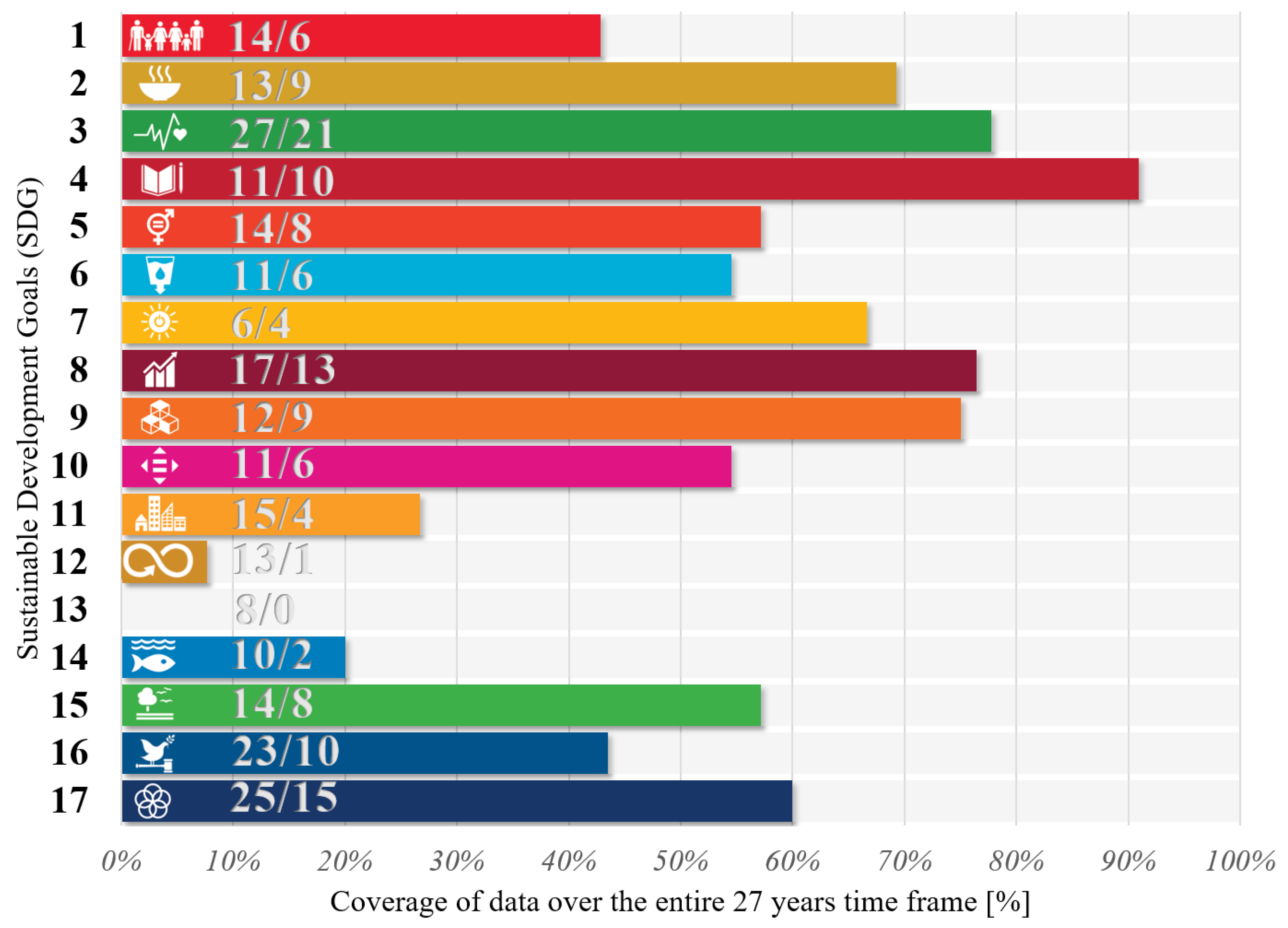
Figure 3.
The worldwide availability of indicators containing records for at least 10 years in the Global SDG Indicators Database [29].
Figure 3.
The worldwide availability of indicators containing records for at least 10 years in the Global SDG Indicators Database [29].
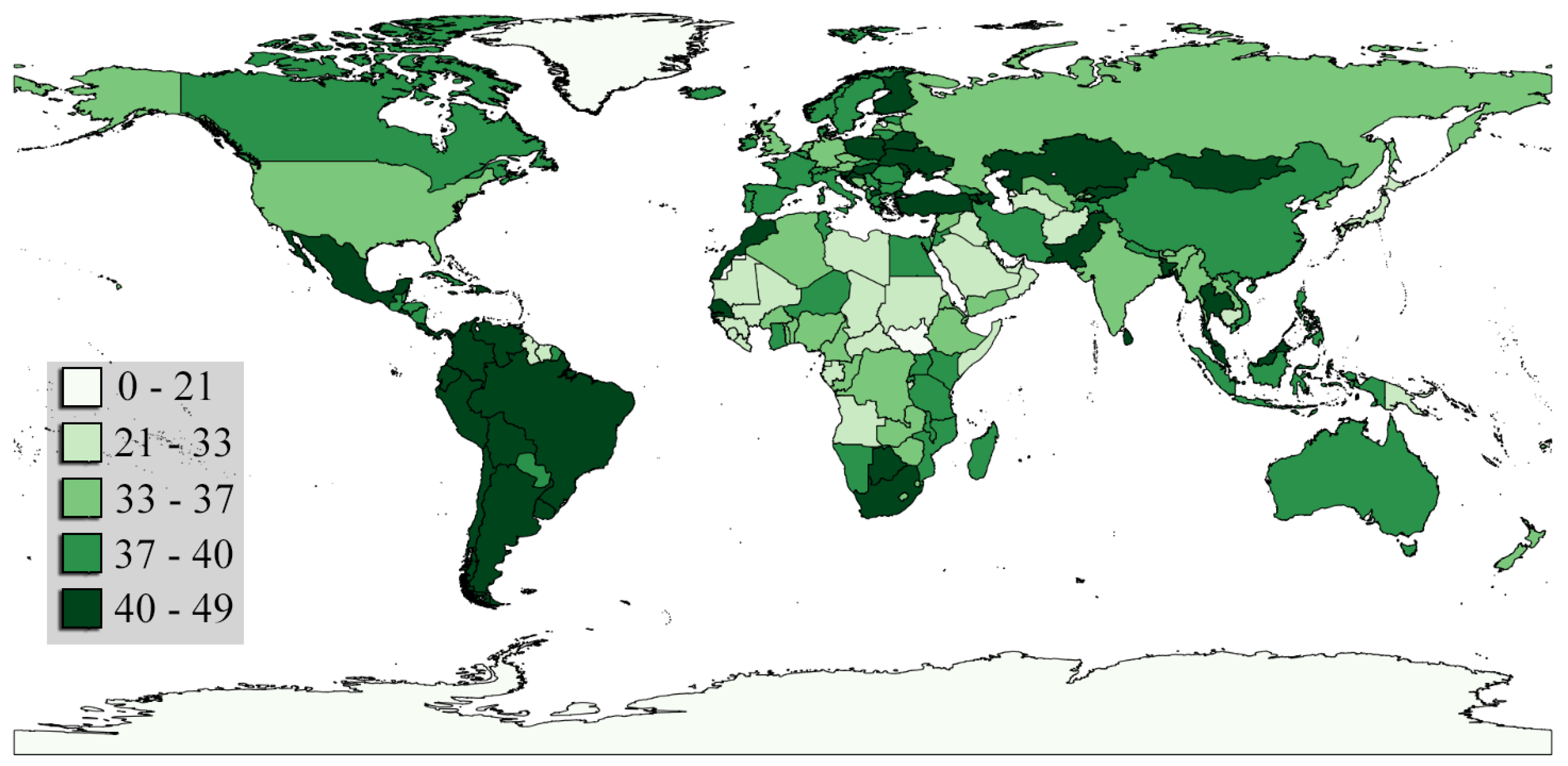
Figure 4.
The algorithm for the choice of the applied causality analysis method. I(0) and I(1) refer to variables integrated in the order of zero and one, respectively.
Figure 4.
The algorithm for the choice of the applied causality analysis method. I(0) and I(1) refer to variables integrated in the order of zero and one, respectively.
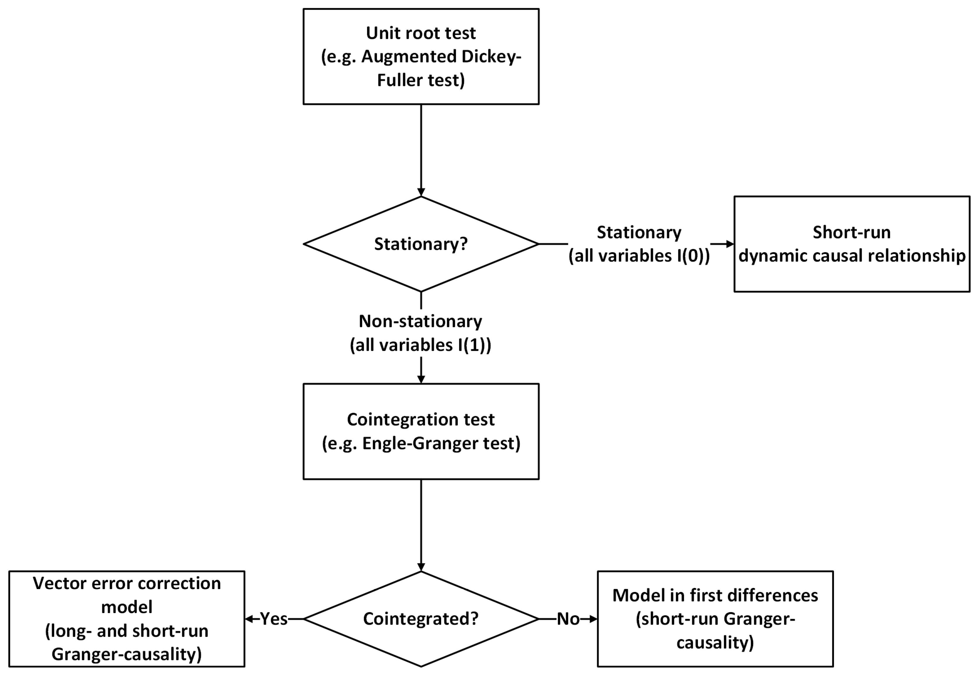
Figure 5.
The stock-and-flow diagram of the World3 model taken from [55]. The enlarged part describes the flow of causality in the ageing of the population (numbers are the ages in years). This flow of causality is nicely revealed by the presented methodology, as described in the following.
Figure 5.
The stock-and-flow diagram of the World3 model taken from [55]. The enlarged part describes the flow of causality in the ageing of the population (numbers are the ages in years). This flow of causality is nicely revealed by the presented methodology, as described in the following.

Figure 6.
The predicted (caused) and the causal variable, as well as the one-step-ahead prediction using the fitted model. The term indicates that one time-lag is applied for the caused variable and zero time-lag for the causal variable (the data point in the contemporaneous time step as the predicted variable).

Figure 7.
A directed network-based representation of the revealed significant causal relationships between the analysed variables of the World3 model. The strong degree of interconnectedness between the variables is clearly visible using the network-based representation.
Figure 7.
A directed network-based representation of the revealed significant causal relationships between the analysed variables of the World3 model. The strong degree of interconnectedness between the variables is clearly visible using the network-based representation.

Figure 8.
The network obtained by the transitive reduction of the network presented in Figure 7. The “flow of causality” is easily traceable in this representation.
Figure 8.
The network obtained by the transitive reduction of the network presented in Figure 7. The “flow of causality” is easily traceable in this representation.
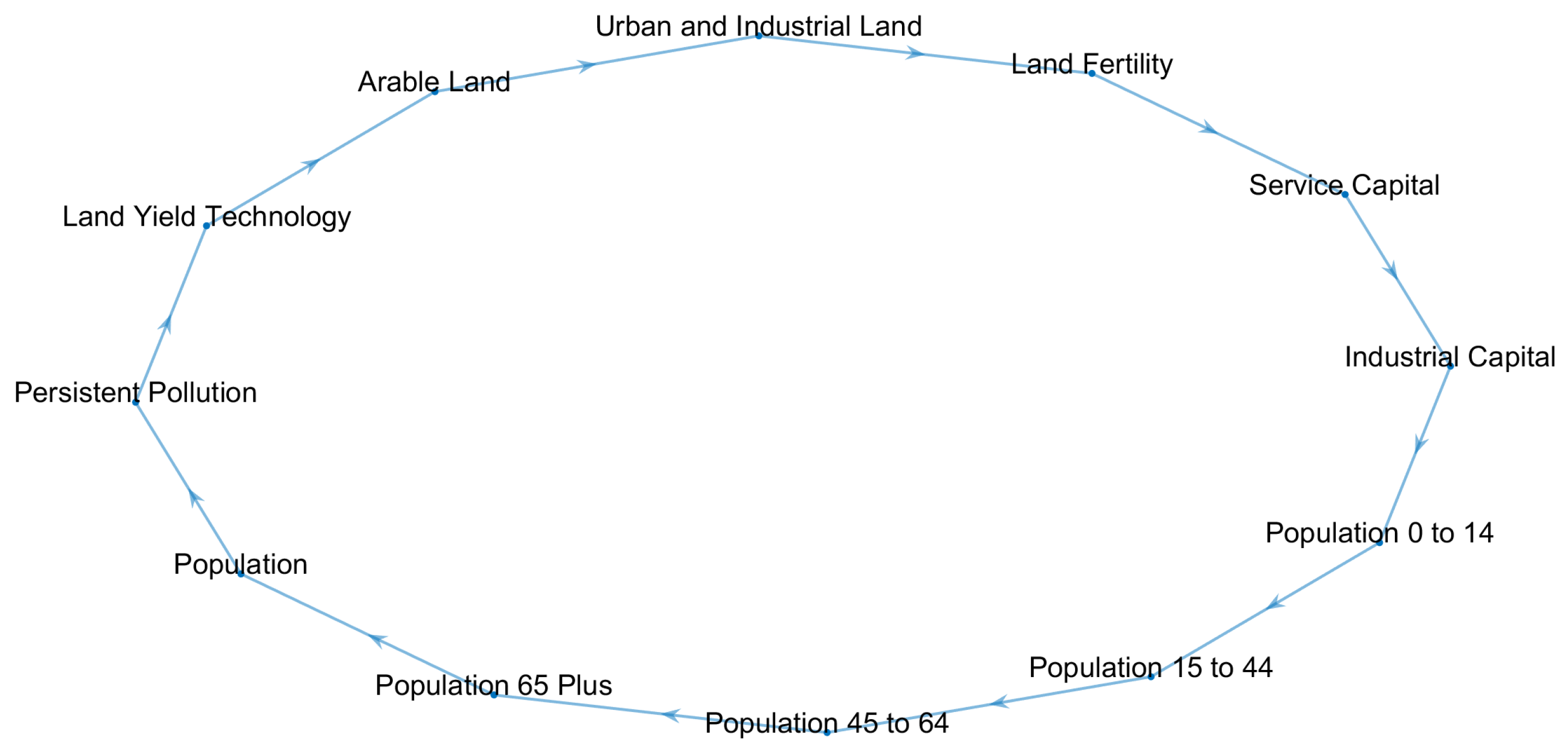
Figure 9.
Minimum spanning tree of a graph representation of the correlation matrix. The indicator IDs follow the “CGGTTII” structure, where GG shows the number of the goal, TT represents the target assigned to the goal, and II shows the reference number of the indicator. The colour of the nodes represent the goal that is associated with the given indicator to highlight that the SDGs are highly interdependent. The original network, its node and edge lists and the description of the Indicator IDs are available at the website of the authors (see Supplementary Materials at www.abonyilab.com).
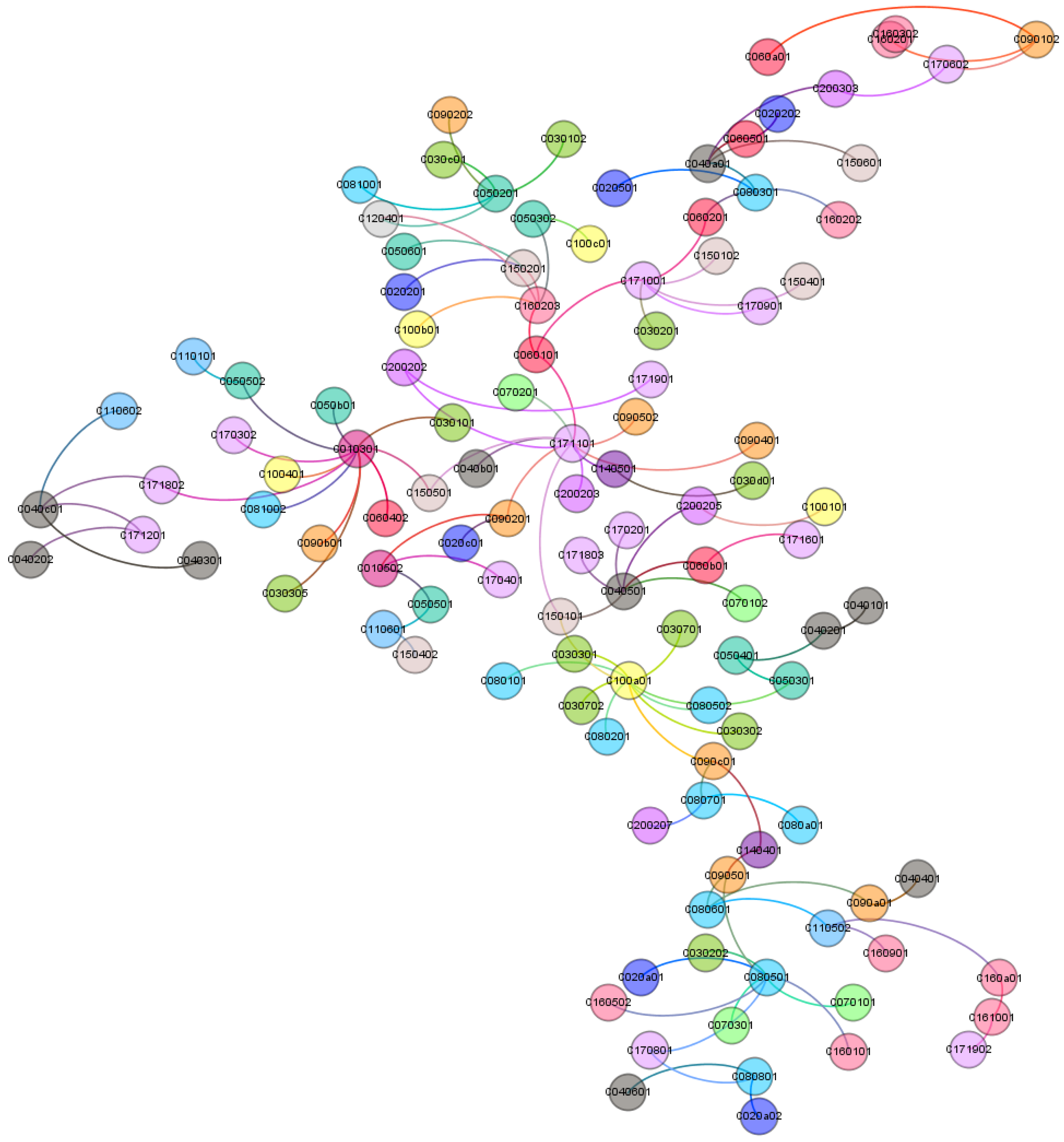
Figure 10.
The availability of the indicators at the different steps of the analysis. The upper part of the figure shows the availability of the individual indicators, while the bottom part illustrates how the causal connection of the indicator pairs was analysed. The numbers in parenthesis show the number of indicators that passed the related statistical tests but not the threshold of the associated p-value. SR and LR stand for short- and long-run causality, respectively.
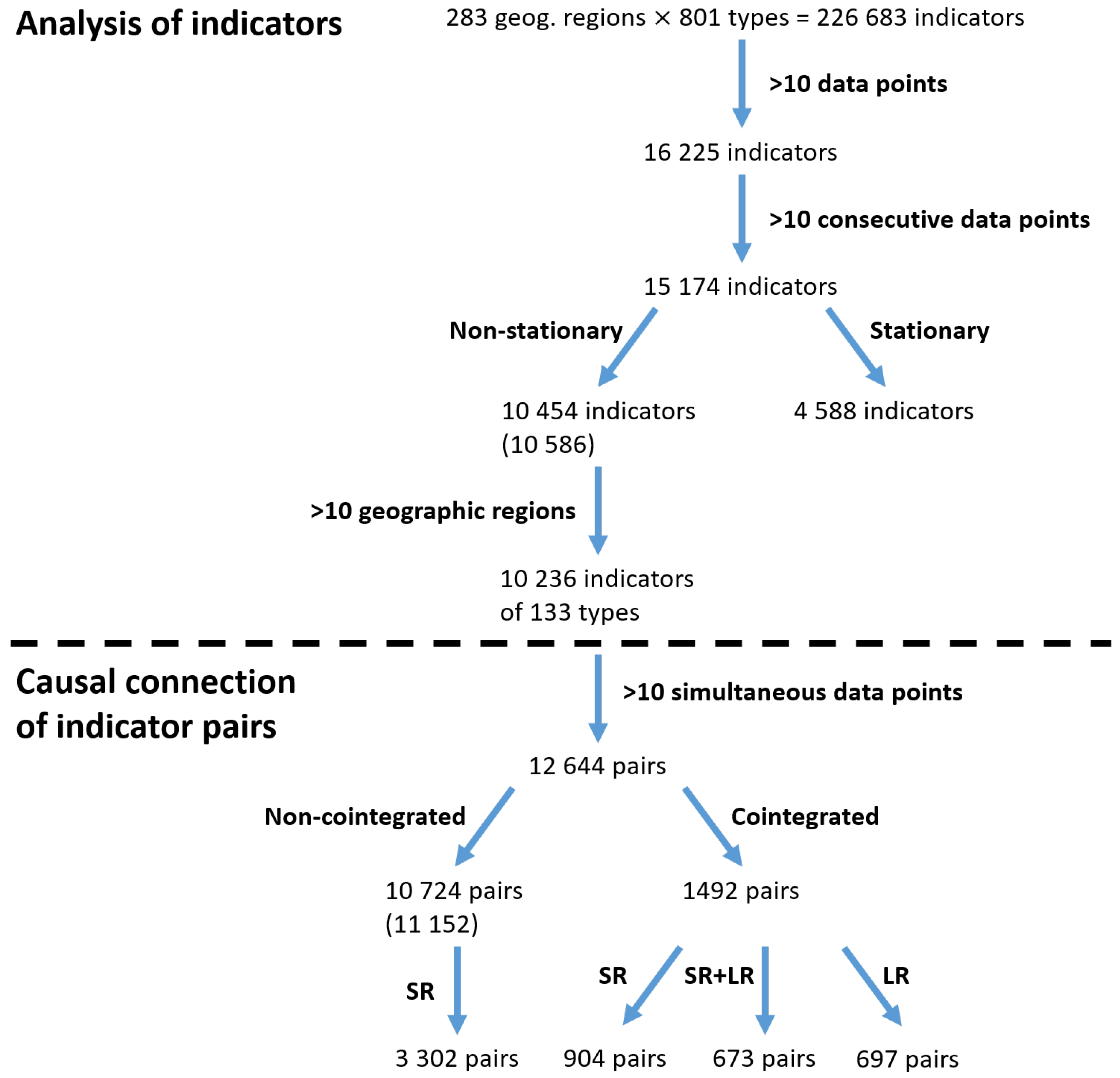
Figure 11.
The network of the revealed short-run causal relationships between the sustainability indicators of Turkey (a) and its transitive reduction (b). The central role of the indicator “Proportion of population below the international poverty line, by sex, age, employment status and geographical location (urban/rural)” (Indicator ID: C010101) is visible. The indicators assigned to the different Indicator IDs are shown in Table 5.
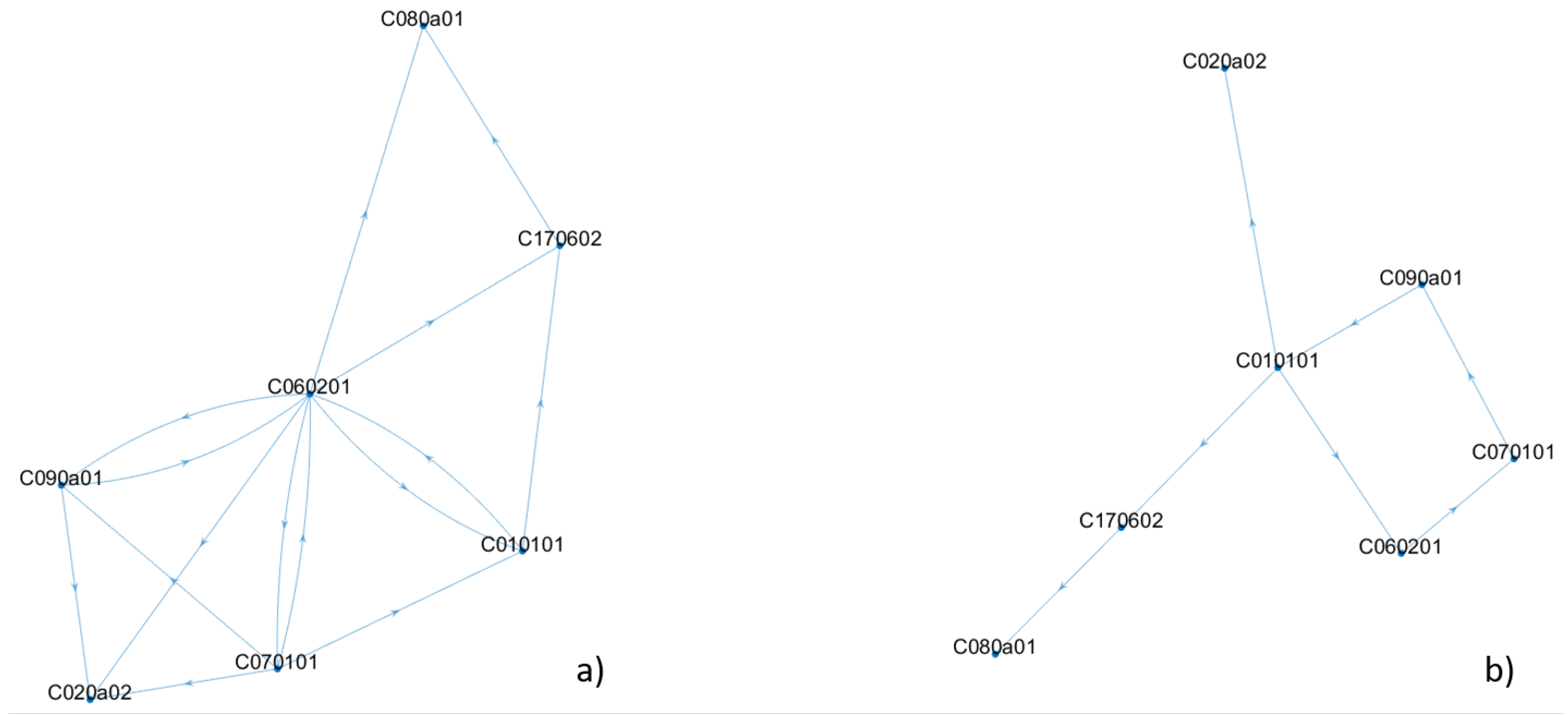
Figure 12.
Network-based representation of the most significant causalities that were identified between the indicators of at least 10 regional datasets (a) and its transitive reduction (b). The indicators assigned to the different Indicator IDs are shown in Table 5.
Figure 12.
Network-based representation of the most significant causalities that were identified between the indicators of at least 10 regional datasets (a) and its transitive reduction (b). The indicators assigned to the different Indicator IDs are shown in Table 5.
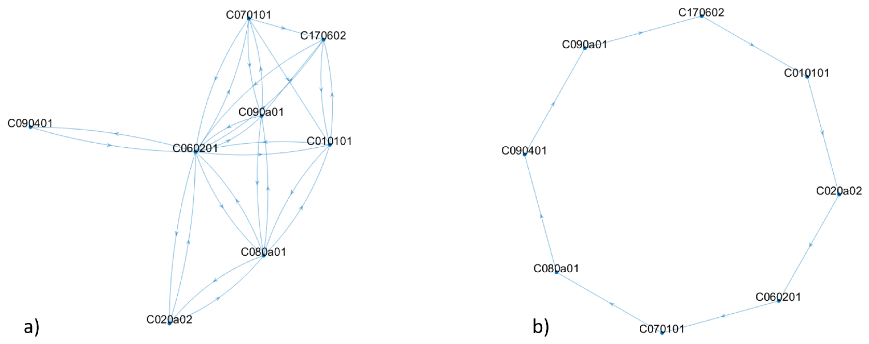

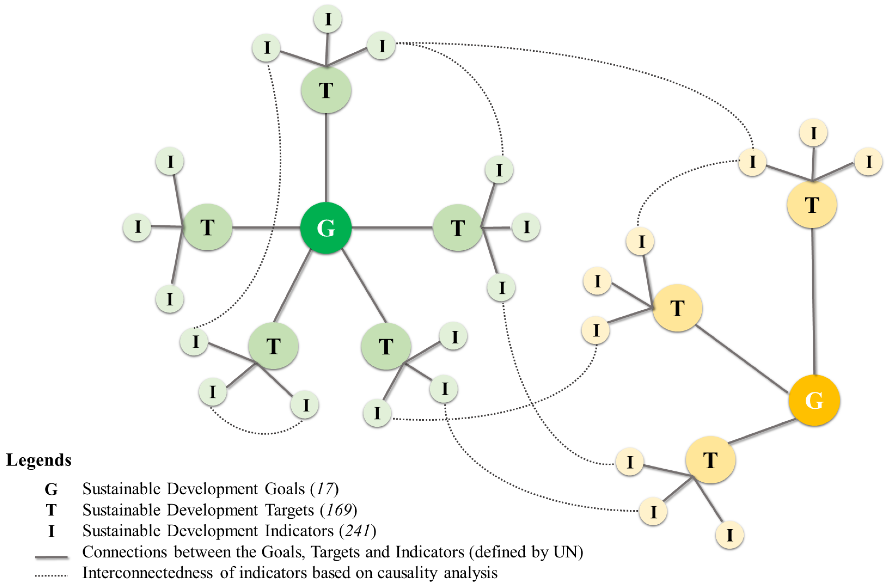
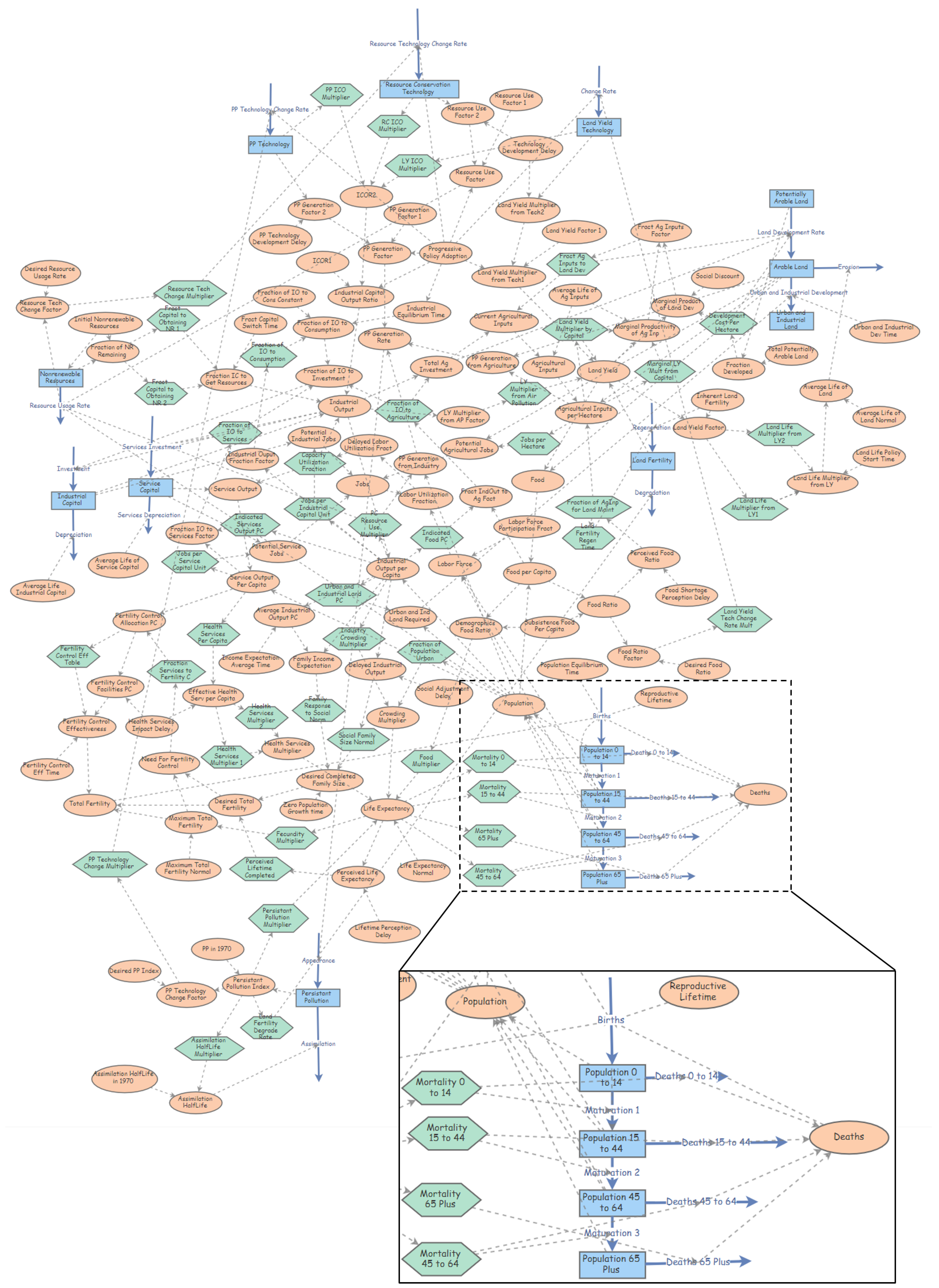
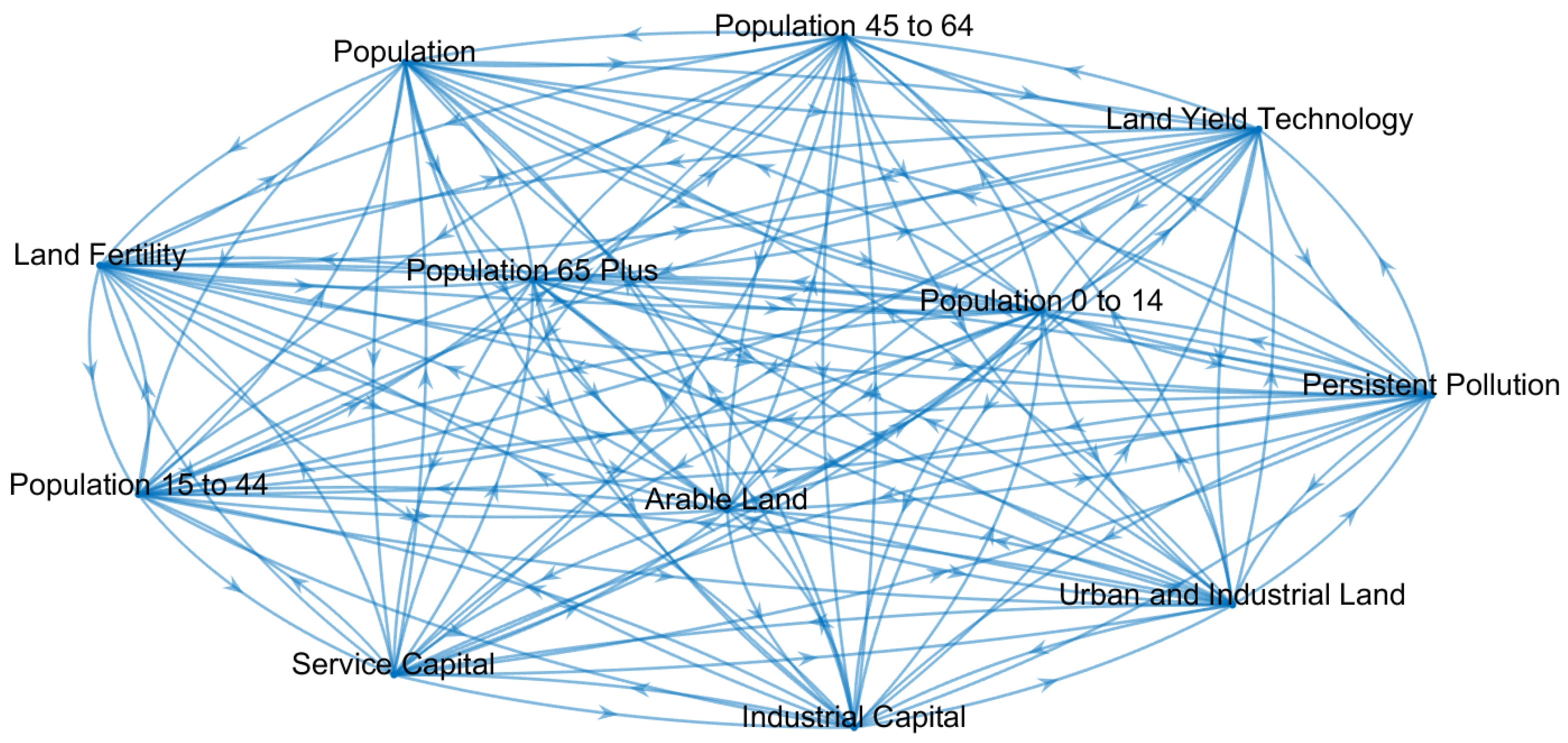
Table 1.
The results of the t- and F-statistics for the analysis of the significance of the term and the fitted parameters, respectively (p = 1, q = 1, contemporaneous y incorporated).
Table 1.
The results of the t- and F-statistics for the analysis of the significance of the term and the fitted parameters, respectively (p = 1, q = 1, contemporaneous y incorporated).
| Cause Variable | Effect Variable | ECT (t-Stats) | Joint Short- and Long-Rung Causality (F-Stats) |
|---|---|---|---|
| Land Yield Technology | Population 0 to 14 | −7.1905 (p < 0.0005) | 44,381 (p < 0.0005) |
Table 2.
The indicator pairs possessing the highest correlation values.
| Indicator Code | Indicator Description | Indicator Code | Indicator Description |
|---|---|---|---|
| C060b01 | Proportion of local administrative units with established and operational policies and procedures for participation of local communities in water and sanitation management | C171601 | Number of countries reporting progress in multi-stakeholder development effectiveness monitoring frameworks that support the achievement of the sustainable development goals |
| C171101 | Developing countries and least developed countries share of global exports | C090201 | Manufacturing value added as a proportion of GDP and per capita |
| C171101 | Developing countries and least developed countries share of global exports | C090401 | emission per unit of value added |
| C171001 | Worldwide weighted tariff-average | C170901 | Dollar value of financial and technical assistance (including through North–South, South–South and triangular cooperation) committed to developing countries |
| C200203 | Domestic material consumption, domestic material consumption per capita, and domestic material consumption per GDP | C171101 | Developing countries and least developed countries share of global exports |
Table 3.
The most important short-run causal connections between the sustainability indicators of Turkey based on their F-statistics.
Table 3.
The most important short-run causal connections between the sustainability indicators of Turkey based on their F-statistics.
| Cause | Description of the Cause | Effect | Description of the Effect |
|---|---|---|---|
| C010101 | Proportion of population below the international poverty line, by sex, age, employment status and geographical location (urban/rural) | C060201 | Proportion of population using safely managed sanitation services, including a hand-washing facility with soap and water |
| C060201 | Proportion of population using safely managed sanitation services, including a hand-washing facility with soap and water | C010101 | Proportion of population below the international poverty line, by sex, age, employment status and geographical location (urban/rural) |
| C010101 | Proportion of population below the international poverty line, by sex, age, employment status and geographical location (urban/rural) | C170602 | Fixed Internet broadband subscriptions per 100 inhabitants, by speed |
| C070101 | Proportion of population with access to electricity | C010101 | Proportion of population below the international poverty line, by sex, age, employment status and geographical location (urban/rural) |
| C060201 | Proportion of population using safely managed sanitation services, including a hand-washing facility with soap and water | C020a02 | Total official flows (official development assistance plus other official flows) to the agriculture sector |
Table 4.
The most important and significant causalities that were identified between the indicators of at least 10 regional datasets.
Table 4.
The most important and significant causalities that were identified between the indicators of at least 10 regional datasets.
| Cause | Description of the Cause | Effect | Description of the Effect |
|---|---|---|---|
| C060201 | Proportion of population using safely managed sanitation services, including a hand-washing facility with soap and water | C090a01 | Total official international support (official development assistance plus other official flows) to infrastructure |
| C090a01 | Total official international support (official development assistance plus other official flows) to infrastructure | C060201 | Proportion of population using safely managed sanitation services, including a hand-washing facility with soap and water |
| C060201 | Proportion of population using safely managed sanitation services, including a hand-washing facility with soap and water | C080a01 | Aid for Trade commitments and disbursements |
| C060201 | Proportion of population using safely managed sanitation services, including a hand-washing facility with soap and water | C010101 | Proportion of population below the international poverty line, by sex, age, employment status and geographical location (urban/rural) |
| C010101 | Proportion of population below the international poverty line, by sex, age, employment status and geographical location (urban/rural) | C060201 | Proportion of population using safely managed sanitation services, including a hand-washing facility with soap and water |
| C060201 | Proportion of population using safely managed sanitation services, including a hand-washing facility with soap and water | C020a02 | Total official flows (official development assistance plus other official flows) to the agriculture sector |
Table 5.
The importance of the indicators according to the out-closeness node centrality metric.
| Indicator Code | Indicator Description | Node Centrality |
|---|---|---|
| C060201 | Proportion of population using safely managed sanitation services, including a hand-washing facility with soap and water | 0.143 |
| C070101 | Proportion of population with access to electricity | 0.100 |
| C080a01 | Aid for Trade commitments and disbursements | 0.100 |
| C090a01 | Total official international support (official development assistance plus other official flows) to infrastructure | 0.100 |
| C010101 | Proportion of population below the international poverty line, by sex, age, employment status and geographical location (urban/rural) | 0.091 |
| C020a02 | Total official flows (official development assistance plus other official flows) to the agriculture sector | 0.083 |
| C170602 | Fixed Internet broadband subscriptions per 100 inhabitants, by speed | 0.083 |
| C090401 | CO2 emission per unit of value added | 0.077 |
© 2018 by the authors. Licensee MDPI, Basel, Switzerland. This article is an open access article distributed under the terms and conditions of the Creative Commons Attribution (CC BY) license (http://creativecommons.org/licenses/by/4.0/).
Share and Cite
MDPI and ACS Style
Dörgő, G.; Sebestyén, V.; Abonyi, J. Evaluating the Interconnectedness of the Sustainable Development Goals Based on the Causality Analysis of Sustainability Indicators. Sustainability 2018, 10, 3766. https://doi.org/10.3390/su10103766
AMA Style
Dörgő G, Sebestyén V, Abonyi J. Evaluating the Interconnectedness of the Sustainable Development Goals Based on the Causality Analysis of Sustainability Indicators. Sustainability. 2018; 10(10):3766. https://doi.org/10.3390/su10103766
Chicago/Turabian StyleDörgő, Gyula, Viktor Sebestyén, and János Abonyi. 2018. "Evaluating the Interconnectedness of the Sustainable Development Goals Based on the Causality Analysis of Sustainability Indicators" Sustainability 10, no. 10: 3766. https://doi.org/10.3390/su10103766
Note that from the first issue of 2016, this journal uses article numbers instead of page numbers. See further details here.