Surplus or Deficit? Spatiotemporal Variations of the Supply, Demand, and Budget of Landscape Services and Landscape Multifunctionality in Suburban Shanghai, China

Abstract

Landscape services are inevitably interlinked with human wellbeing. It is essential to assess landscape services and multifunctionality from both supply and demand points of view toward sustainable landscape management. This study focused on the spatiotemporal variations of the supply, demand, and budget of landscape services in suburban Shanghai, China, including crop production, nutrient regulation, air-quality regulation, soil-erosion regulation, water purification, and recreation and aesthetical value. A new index landscape multifunctionality budget (B_MFI) was developed, integrating the budget status of surplus and deficit with landscape management. Spatial autocorrelation analysis and regression analysis were conducted to identify spatial agglomeration and influencing factors of B_MFI. Pronounced spatiotemporal heterogeneity of landscape services was observed. B_MFI was in surplus status in 2005 and 2010, but turned to deficit in 2015. Landscape service budgets generally followed the spatial pattern of positive in the west and negative in the east. Budget deficits covered half of the villages in 2015, which were mainly situated near central Shanghai with high population density, high average income, and a fragmented and less diverse landscape pattern. Rapid urban sprawl and the following land-cover changes are the main drivers for the spatiotemporal variations. Landscape function zoning with effective economic development and ecological conservation policies can comprehensively improve the competitiveness achieving sustainable future.

1. Introduction

Landscape services contributing to human wellbeing in terms of economic, sociocultural, and ecological benefits [1,2,3,4] are vital for achieving self-sustaining human–environmental systems and sustainable utilization of natural capital [5]. Landscape services are defined as “the goods and services provided by landscape to satisfy human needs, directly or indirectly” [4,6]. Currently, although the term “landscape services” is considered to be generally synonymous with “ecosystem services”, and the two can substitute for each other in most cases [6,7,8,9,10,11,12,13], we prefer the term “landscape services”, which is more appropriate and appealing [14,15] in this paper for local actors, as it infers pattern–process interactions and unites scientific disciplines [4,5,16]. In addition, the term “landscape services” can describe the various benefits provided by both natural and artificial landscapes, while the term “ecosystem services” pays more attention to natural systems [17]. For suburban areas with intensive natural process and human activities, using the term “landscape services” is more suitable for collaborative decision-making. At any given location, usually more than one landscape service is provided [15]. This refers to the phenomenon of landscape multifunctionality, whereby the landscape actually or potentially provides multiple material and immaterial goods or services to satisfy social needs [18]. Promoting multifunctionality became an important direction in landscape service research and this interdisciplinary concept provides a suitable platform in both theory and practice to combine or disentangle effects of multiple environmental stressors acting on the landscape from a sustainability perspective [19,20].

Landscape services and landscape multifunctionality exhibit significant spatial and temporal heterogeneity [21,22,23,24]. The importance of assessing and mapping multiple landscape services is increasingly recognized in recent studies [25,26,27], as quantitative and visible illustrations are essential for realizing successful landscape planning and environmental management [6,13,28]. Progress was made in the evaluation of both landscape services and landscape multifunctionality. Quantification modeling method plays an important role in the assessment [29]. Models can vary from simple expert-based scoring systems to complex ecological models which simulate the planetary cycles of carbon, nitrogen, and water [30]. Some scientists calculated landscape services via indirect measurements such as net primary productivity (NPP) and normalized difference vegetation index (NDVI) [31,32]. Geographic information system (GIS) analysis through spatiotemporal indicators is also very useful to address land diagnosis and assessment, providing a numerical and objective perspective [33]. Assigning monetary values to landscape services is a hot issue [34,35,36]. Nevertheless, Burkhard et al. [37,38] argued that the outcomes of monetary approaches are often disappointing due to the focus on economics and the lack of appropriate pricing methods, especially for non-marketed goods and services [39]. Landscape services variations are tightly bound to land use and cover change, which is driven by the interaction in space and time between biophysical and human dimensions [40], and consequently impacts landscape services provided to human society. Land use and cover change analysis is effective for understanding and explaining the causes and consequences of land-use dynamics and for estimating the related impacts of changes on landscape [41,42]. Approaches including land-use models, indicator-based methods, and scenario analysis are widely used in the assessment of land use and cover change and its spatial pattern [43], in order to support the evaluation of landscape services and to promote landscape planning and policy.

However, the assessment and mapping of landscape services mostly focuses on the supply side and few studies mapped the demand for landscape services [44,45], which is more difficult than doing so for supply, despite the widely acknowledged significance of including the demand side or social preference into the assessment [46,47,48,49]. Landscape is the result of and the medium for interaction between human and nature [50] and landscape services are shaped by both the landscapes and their users. Inclusion of the demand side in the assessment is assumed to identify the mismatch of landscape service delivery, enhance the engagement of stakeholders, and increase policy relevance and practical application of the landscape service concept in operational management [51,52,53,54].

Landscape service budgets are computed by subtracting the demand value from the supply value. The budget surplus and deficit of landscape services can help assess the dependence of a region on service imports or its potential to export certain goods and services [38,55]. The studies integrating multifunctionality with budget and further identifying its influencing factors are rather rare because supply and demand indicators are not directly comparable. Landscape services are driven by a variety of demographic, economic, cultural, and biophysical processes. Several studies evaluated how socioeconomic factors interact with the spatial differences between the supply and demand separately for multiple ecosystem services [44,56,57,58]. For a region suffering from a shortage of land resources, multifunctionality is an objective attribute and determines its development [59], which is often neglected by policy-makers. Therefore, assessing the uneven spatiotemporal distribution of the surplus and deficit of landscape multifunctionality budget and identifying the influencing factors are of great significance to raise awareness and improve decision-making for the allocation of resources among computing demands. Since the economic reform and opening-up policy was put forward in the late 1970s, China achieved tremendous development and rapid urbanization, and intensive human activities associated with significant land-use changes triggered noticeable impacts on landscape patterns, processes, and functions [60,61]. As the interface between urban settlements and rural hinterlands, suburban areas are characterized by complex landscape patterns [33,62,63] and multiple landscape service demands. Shanghai is the chief metropolis in China, and Qingpu is a representative suburban district where challenges and opportunities are faced as it currently undergoes rapid urban sprawl. The assessment of landscape service supply, demand, and budget should be included in spatial planning and landscape decision-making in order to identify priority regions for effective management actions [64,65].

Burkhard et al. [38] proposed a matrix based on the experience from many case study areas, linking spatially explicit biophysical landscape units to service supply and demand. The matrices were used in many cases, including China [58,66,67,68]. In this paper, we took Qingpu District, suburban Shanghai as the case study area and applied the adjusted supply–demand matrix from Burkhard et al. [38] as the basis to conduct the assessment and mapping. The main objectives of this study include (1) examining the temporal and spatial variations of the supply, demand, and budget of landscape services and landscape multifunctionality in Qingpu in 2005, 2010, and 2015; (2) on the village level, from the perspective of the landscape multifunctionality budget, identifying hot and cold spots and influencing factors to inform landscape function zoning, support further research, and provide an orientation for landscape management. The workflow of this study is shown in Figure 1.

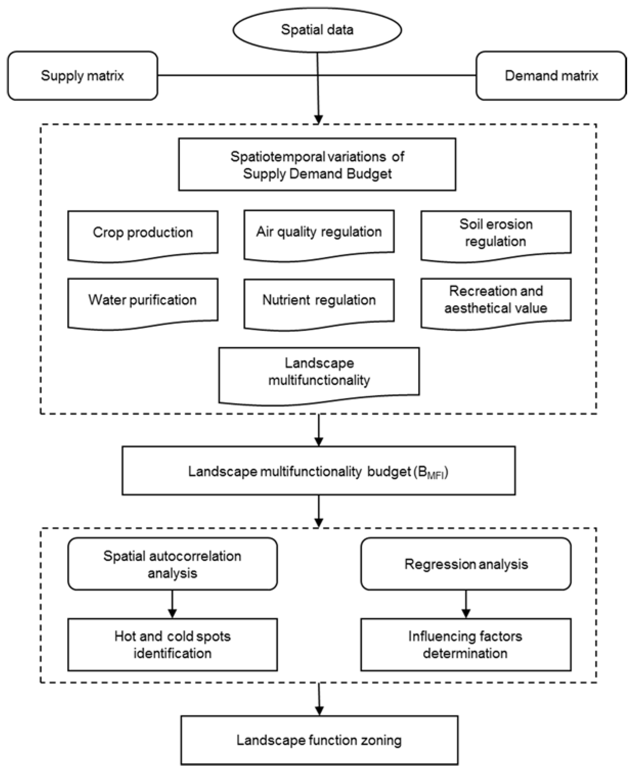
2. Materials and Methods

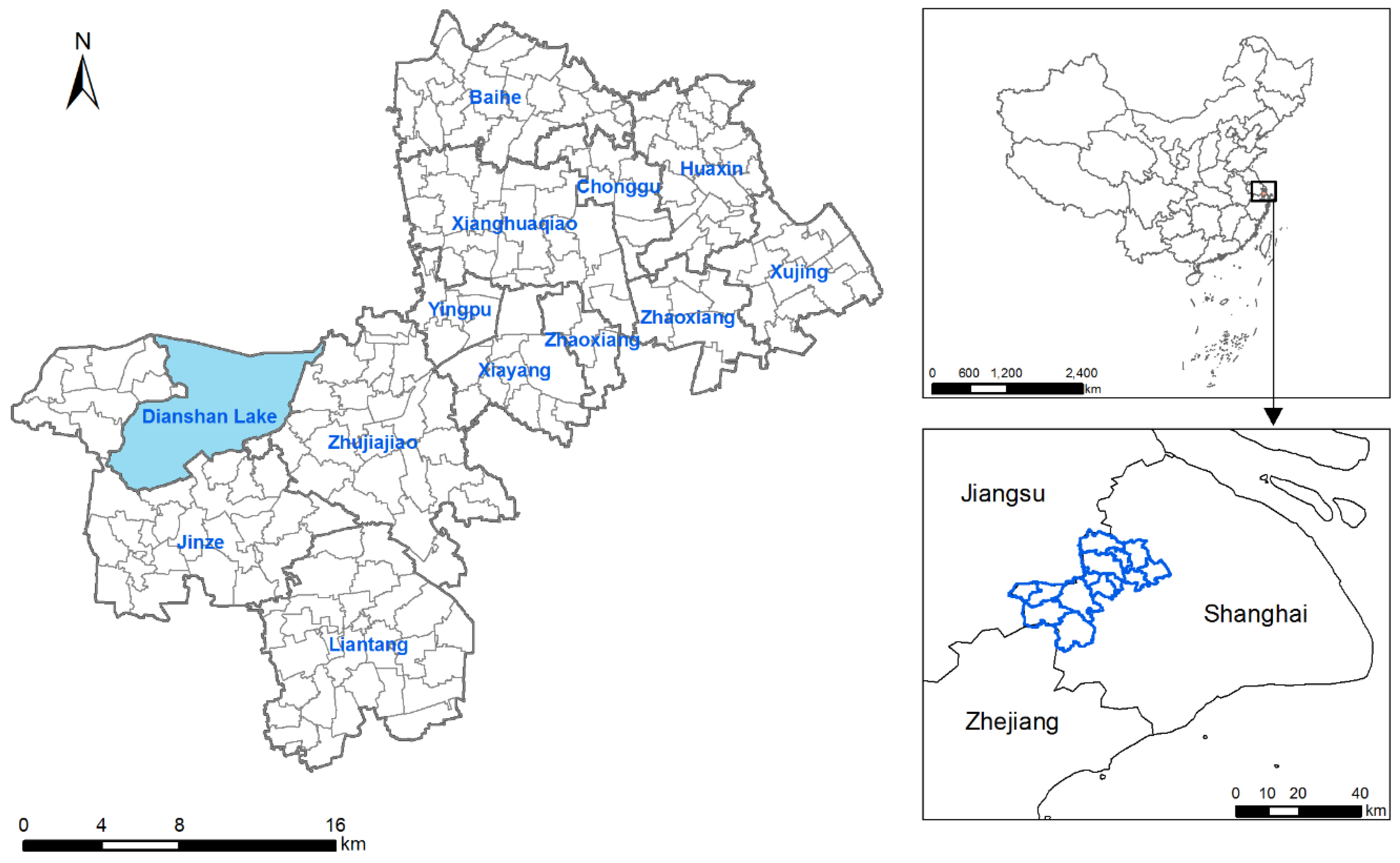
2.1. Study Area

The study was carried out in Qingpu District (included as Supplementary Material), a typical suburban district located on the west side of Shanghai, bordering Zhejiang Province and Jiangsu Province. Qingpu extends over approximately 668 km² and is divided into three sub-districts and eight towns, totally consisting of 185 villages (Dianshan Lake was considered as a village in the analysis). According to Qingpu Planning and Land Resources Bureau (http://prog.shqp.gov.cn/), Xiayang, Yingpu, and Xianghuaqiao are three sub-districts in the urban center of Qingpu, with Zhujiajiao, Liantang, and Jinze on the west wing, and Baihe, Chonggu, Zhaoxiang, Huaxin, and Xujing on the east wing (Figure 2).

Shanghai is one of the fastest developing cities in the world and the commercial and financial center of China. As a representative suburban district of the Shanghai metropolis, Qingpu is experiencing rapid urbanization. In 2015, the resident population of Qingpu was 1.21 million, a 64% increase from 2005 [69,70]. Urban sprawl significantly changed the land-use and land-cover patterns in Qingpu, and the demand for landscape services increased. Qingpu has a humid subtropical climate and most of the region is characterized by low and open terrain. The climate and topography give advantages to agriculture development, which is important for the urban development of Shanghai. In 2015, Qingpu’s gross domestic product (GDP) was 87.82 billion yuan, which accounted for 3.5% of Shanghai’s overall GDP [70,71], while the proportion of Qingpu’s primary industry to Shanghai’s primary industry was 8.1%. Qingpu has abundant natural and cultural landscapes attracting tourists from the surrounding cities. Dianshan Lake is the most important water body in this area and is one of the major drinking water sources for Shanghai as well, and Qingpu implements strict surface water quality standards. The computing demands for economic development and ecological conservation make Qingpu a typical suburban district to conduct landscape service research.

2.2. Data Source

The land-cover data in 2005 and 2010 were produced by the Chinese Academy of Sciences through interpretation of the Landsat thematic mapper (TM) or enhanced TM (ETM) images at a 30-m resolution. The overall accuracy of classification with ground-based survey data was over 90% [72]. As for 2015, the Landsat image acquired on 3 August 2015 was collected from the Geospatial Data Cloud Platform [73]. Using ENVI 4.8, the remote-sensing image was interpreted by supervised classification combined with visual interpretation to produce the land-cover map of Qingpu in 2015 with a pixel size of 30 × 30 m. Land cover in this study was classified into five classes considering local expert knowledge: forest, grassland, water bodies, arable land, and built-up area. We collected the field survey data from Qingpu Planning and Land Resources Bureau to evaluate the classification, and the accuracy was also over 90%. Socioeconomic data on village scale were obtained from Qingpu Statistical Bureau and Qingpu Agriculture Committee.

2.3. Calculation and Mapping of Landscape Services

Burkhard et al. [37,38] proposed a clear expert-based concept to map ecosystem service supply, demand, and budget, which is applicable at different scales for various case study regions. In the evaluation matrices, 44 land-cover types are linked with 29 supplies and 22 demands of landscape services. The value ranging from 0 to 5 means the relevance of this land cover to provide or require the corresponding service. According to the biophysical and socioeconomic context of Qingpu, six highly relevant landscape services were evaluated and mapped: (1) crop production, (2) nutrient regulation, (3) air-quality regulation, (4) soil-erosion regulation, (5) water purification, and (6) recreation and aesthetical value, covering production function, ecological function, and aesthetical function of landscape.

According to the local circumstances of Qingpu, we made an adjustment of the original matrices (

Table 1. Adjusted matrix of the relevance of landscape service supply and demand.

	Supply					Demand
	Forest	Grassland	Water Bodies	Arable Land	Built-Up Area	Forest	Grassland	Water Bodies	Arable Land	Built-Up Area
CP	0	0	0	5	0	0	0.3	0	1	5
NR	5	3.8	2	0	0	0	0	0	3	1
AQR	5	0.3	0	0	0	0	0.3	0	1	5
SER	5	4.1	0	0	0	0	0	0	2	1
WP	5	3.8	1.5	0	0	0	0	0	4.25	1
RAV	5	3	5	1	0	0	1.2	0	0	4

The assessment scale ranges from 0 to 5, which means the relevance from low to high of one land cover to provide or require the corresponding landscape service. CP is crop production, NR represents nutrient regulation, AQR means air-quality regulation, SER is soil-erosion regulation, WP stands for water purification, and RAV is recreation and aesthetical value.

) with participation of stakeholders and local experts. The entries of the two matrices were determined following a four-stage process. Firstly, four authors from China Agricultural University discussed the appropriate extrapolative approaches and decided to assign a score for each entry based on the original matrices using six steps. (1) The value assigned to forest is the average of broad-leaved forest, coniferous forest, and mixed forest in CORINE land-cover classes. (2) According to the statistical yearbook of Qingpu, the proportion of natural grassland to grassland is around 70%, and green urban area accounts for 30%; therefore, the value assigned to grassland is the area-weighted average value of natural grassland and green urban area in the original matrices. (3) The value for water bodies is the average of water bodies and water courses in the original matrices. (4) Non-irrigated arable land accounts for about 15% of arable land in Qingpu, and permanently irrigated arable land is 85%; thus, the supply and demand value assigned to arable land is the area-weighted average. (5) The value assigned to built-up area is the same as continuous urban fabric. (6) The matrices were finally determined after several rounds of discussions with five researchers from China Agricultural University and two local technicians in Qingpu, who are familiar with the local conditions. Secondly, we interviewed five experts with relevant landscape research background from China Agricultural University to provide updates on the matrix entries independently. Subsequently, two technicians (one from Qingpu Environmental Protection Bureau and one from Qingpu Agricultural Committee) who are familiar with local conditions and environmental issues in Qingpu were interviewed. A pre-discussion with farmers, and rural and urban dwellers was held by the technicians before the interview. They were given the explanation of each landscape service and were provided with both the original and the extrapolative matrices; the technicians drew the conclusions from the stakeholders’ opinions for the collaboration with stakeholders [74] to make the matrices coherent with local circumstances. The consistent matrices were finally agreed upon after the panel discussions together with four authors, five researchers from China Agricultural University, and two local technicians in Qingpu. The matrices corresponding to land cover specific to certain landscape service, obtained from the extrapolation approach combined with local expert knowledge and stakeholder participation, are the foundation of the methodology.

The supply, demand, and budget of single landscape service were calculated with the following equations:

$$S_i=\frac{{\displaystyle \sum _{j=1}^{5}S{X}_{ij}}\cdot A_j}{A_t},$$

(1)

$$D_i=\frac{{\displaystyle \sum _{j=1}^{5}D{X}_{ij}\cdot A_j}}{A_t},$$

(2)

$$B_i=S_i-D_i,$$

(3)

where i is the landscape service, j is the land-cover type, A_j is the area of the jth landscape unit in the study scale, and A_t is the total area of the study scale; SX_ij and DX_ij are the values of the supply and demand of each land-cover type in Table 1.

For the quantification of landscape multifunctionality, in this paper, air-quality regulation, nutrient regulation, soil-erosion regulation, and water purification were considered as ecological services with the same weight. Crop production, and recreation and aesthetical value were regarded as a production service and aesthetical service, respectively. Landscape multifunctionality is the simple unweighted summation of production service, ecological service, and aesthetical service. We propose an index of landscape multifunctionality budget (B_MFI) that was calculated with the following equations:

$$S_{MFI}=S_{CP}+S_{RAV}+(S_{NR}+S_{AQR}+S_{SER}+S_{WP})/4,$$

(4)

$$D_{MFI}=D_{CP}+D_{RAV}+(D_{NR}+D_{AQR}+D_{SER}+D_{WP})/4,$$

(5)

$$B_{MFI}=B_{CP}+B_{RAV}+(B_{NR}+B_{AQR}+B_{SER}+B_{WP})/4=S_{MFI}-D_{MFI},$$

(6)

where S, D, and B represent supply, demand, and budget, respectively. MFI is the multifunctionality index. Other abbreviations were explained above.

The matrices and equations were applied at three different spatial scales: Qingpu District, 300 × 300 m fishnet, and village. (1) To explore the temporal variation of Qingpu, we calculated the supply, demand, and budget value of each landscape service and landscape multifunctionality index in the years 2005, 2010, and 2015. (2) A service map is not only the reclassification of the landscape units according to the matrix, but also a synthetic visualization of the landscape elements. In order to spatialize the supply, demand, and budget of landscape services and to identify the spatial heterogeneity in 2015, 300 × 300 m fishnets across the study area were created, and the value of each fishnet was calculated using the equations above. Each fishnet may contain more than one land-cover type. Different sizes of the fishnet were tested, ranging from 100 m to 500 m, with increasing steps of 50 m, and 300 m was eventually selected. An increase in the fishnet size decreases the spatial resolution of the map, while smaller fishnets do not contain enough information for the map. (3) For further analysis of the landscape services with other indicators in 2015, B_MFI was calculated at the village level (Dianshan Lake was considered as a village) in Qingpu using the area-weighted method stated above. All computations were finished through the raster calculator and zonal statistics in the ArcGIS 10.3 software.

2.4. Data Analysis at the Village Level

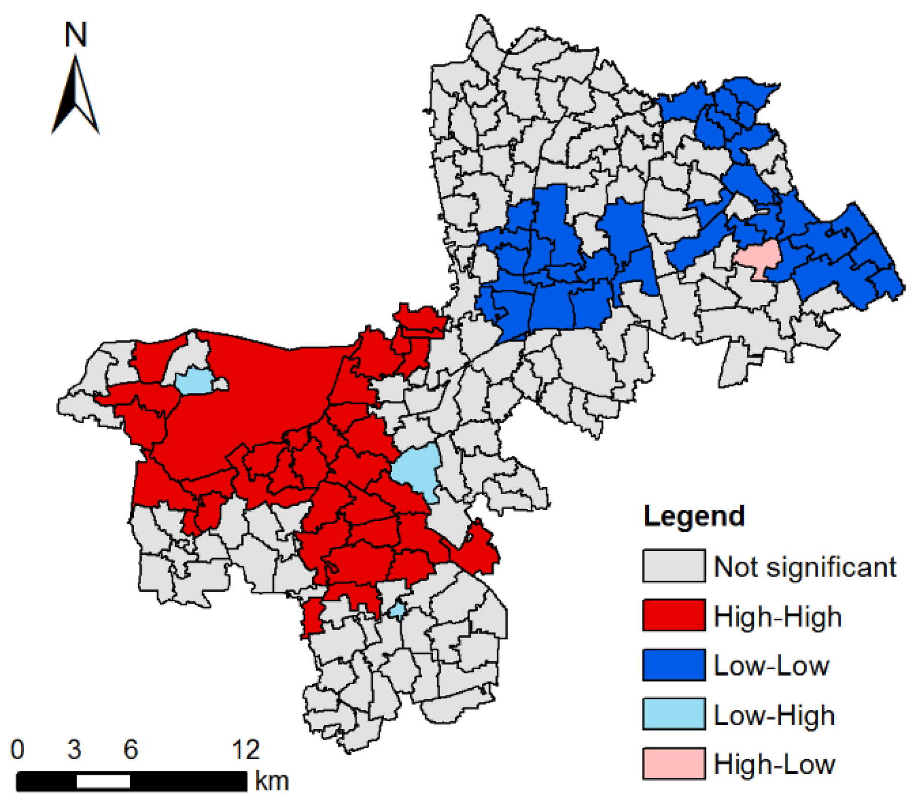
2.4.1. Spatial Autocorrelation Analysis

To explore the spatial agglomeration of landscape multifunctionality budget in Qingpu, spatial autocorrelation analysis was carried out. Global spatial autocorrelation reflects the overall clustering of the data, which can be measured by global Moran’s I tool using the following formula:

$$I=\frac{n}{{\displaystyle \sum _{i=1}^n{\displaystyle \sum _{j=1}^n{w}_{ij}}}}\frac{{\displaystyle \sum _{i=1}^n{\displaystyle \sum _{j=1}^n{w}_{ij}\left(x_i-\overline{x}\right)\left(x_j-\overline{x}\right)}}}{{\displaystyle \sum _{i=1}^n{\left(x_i-\overline{x}\right)}^2}},$$

(7)

where n is the number of spatial units indexed by i and j, x_i and x_j are the values of variable x, $\overline{x}$ is the mean of x, and w_ij is the matrix of spatial weights.

Anselin [75] proposed local indicators of spatial association (LISA) to identify the local patterns of spatial association (local spatial autocorrelation). Local Moran’s I tool used in this paper is a LISA that allows for the decomposition of global Moran’s I tool into the contribution of each spatial unit. The calculation formula is as follows:

$$I_i=\frac{\left(x_i-\overline{x}\right)}{{\displaystyle \sum _i{\left(x_i-\overline{x}\right)}^2/n}}{\displaystyle \sum _j{w}_{ij}\left(x_i-\overline{x}\right)}.$$

(8)

By calculating global Moran’s I and local Moran’s I values with rook contiguity as spatial weights in the Geoda 1.12 software, spatial agglomeration and hot and cold spots of B_MFI were identified. Only when the element had a high (low) value and was also surrounded by elements with similar high (low) values, it was deemed a statistically significant hot (cold) spot.

2.4.2. Regression Analysis of Landscape Multifunctionality with Other Indicators

The relationships between B_MFI and other indicators in 2015 were modeled using linear regression analysis with the SPSS 20.0 software. Three landscape metrics and seven socioeconomic indicators (

Table 2. List of landscape metrics and socioeconomic indicators for the regression analysis.

Criteria	Variables	Unit
Landscape metrics	Edge density (ED)	m/ha
	Shannon’s diversity index (SHDI)	-
	Contagion index (CONTAG)	%
Socioeconomic indicators	Population density (PopDen)	Persons/km2
	Distance to the city center of Shanghai (DisSH)	m
	Distance to the center of Qingpu (DisQP)	m
	Per capita annual income (AI)	Yuan
	Per household arable land area (ALA)	m2/household
	Per household labor force (LF)	#
	Average duration of education per household (Edu)	Year

) were selected and the villages were taken as the observations. Landscape metrics were computed with the land-cover map by the moving window method in the Fragstats 4.2 software, and the window size was 500 × 500 m. This window size was appropriate because it minimized data redundancy and could indicate a suitable distance to reflect distinctive spatial signatures of landscape patterns without missing important details in Qingpu compared with sizes of 100 m, 300 m, 1000 m, and 2000 m that were also considered.

3. Results

3.1. Temporal Variations of Landscape Services from 2005 to 2015

The supply, demand, and budget of landscape services in Qingpu from 2005 to 2015 are shown in

Table 3. Temporal variations of landscape service supply, demand, and budget.

	Supply			Demand			Budget
	2005	2010	2015	2005	2010	2015	2005	2010	2015
CP	3.0232	2.5793	2.3585	1.5001	1.7047	1.9216	1.5232	0.8746	0.4369
NR	0.3975	0.5713	0.5752	1.9928	1.7849	1.7046	−1.5953	−1.2136	−1.1294
AQR	0.1651	0.3298	0.3388	1.5001	1.7047	1.9216	−1.3349	−1.3749	−1.5828
SER	0.1794	0.3585	0.3687	1.3882	1.269	1.2329	−1.2087	−0.9105	−0.8642
WP	0.2372	0.4182	0.4342	2.7486	2.4297	2.2943	−2.5114	−2.0115	−1.86
RAV	1.6796	1.7349	1.6499	0.7199	0.9583	1.1675	0.9597	0.7765	0.4824
MFI	4.9477	4.7336	4.4377	4.1274	4.4601	4.8774	0.8203	0.2734	−0.4397

. In 2005, 2010, and 2015, the supply of crop production was much higher than the other five landscape services, and air-quality regulation was the lowest ranking among the services. Crop production supply decreased by 22%, while the supply of air-quality regulation and soil-erosion regulation more than doubled during the decade. Continuous increases were also observed in nutrient regulation (45%) and water purification (83%). The supply of recreation and aesthetical value climbed from 2005 to 2010, but dropped from 2010 to 2015, with a slight decrement by 1.8% in the decade. The gap between the supply of crop production and that of the other five landscape services narrowed in 2015.

The demands for six landscape services in 2005, 2010, and 2015 were relatively equal compared to the supply side. The demand for crop production and air-quality regulation increased by 28%, and significant growth existed in the demand for recreation and aesthetical value (62%) in the ten years. Meanwhile, there was a constant reduction in the demand for nutrient regulation, soil-erosion regulation, and water purification, reducing by 14%, 11%, and 16%, respectively.

Although the budgets of nutrient regulation, soil-erosion regulation, and water purification increased by 29%, 28%, and 25%, respectively, these services were still in deficit status during the decade. Moreover, the budget of air-quality regulation declined by 18%. The budgets of crop production and recreation and aesthetical value also tightened.

As for landscape multifunctionality, the supply fell by 10%, and contrarily, the demand gradually rose by 18% from 2005 to 2015. Consequently, the supply of landscape multifunctionality exceeded the demand in 2005 and 2010, whereas the budget surplus turned to budget deficit in 2015.

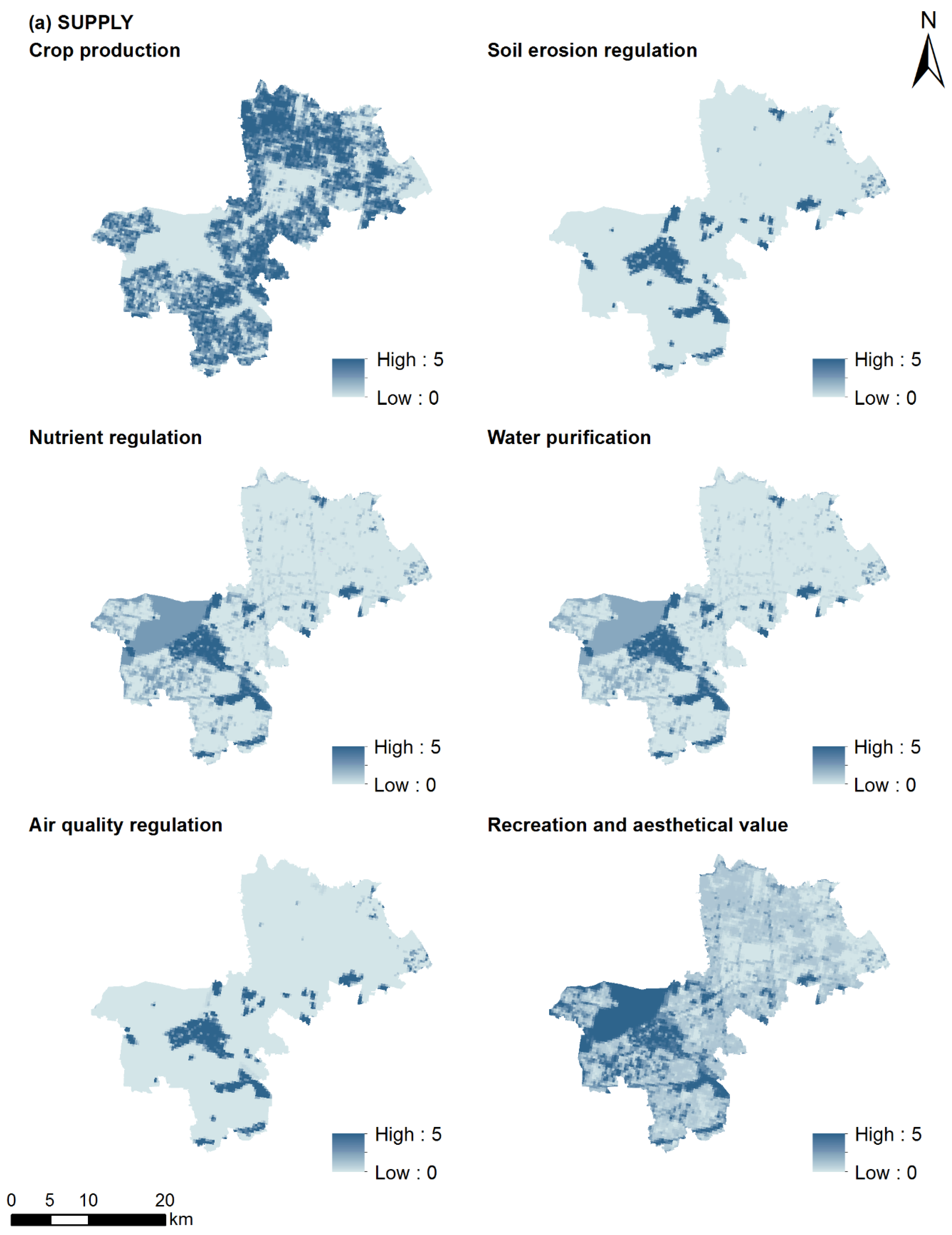
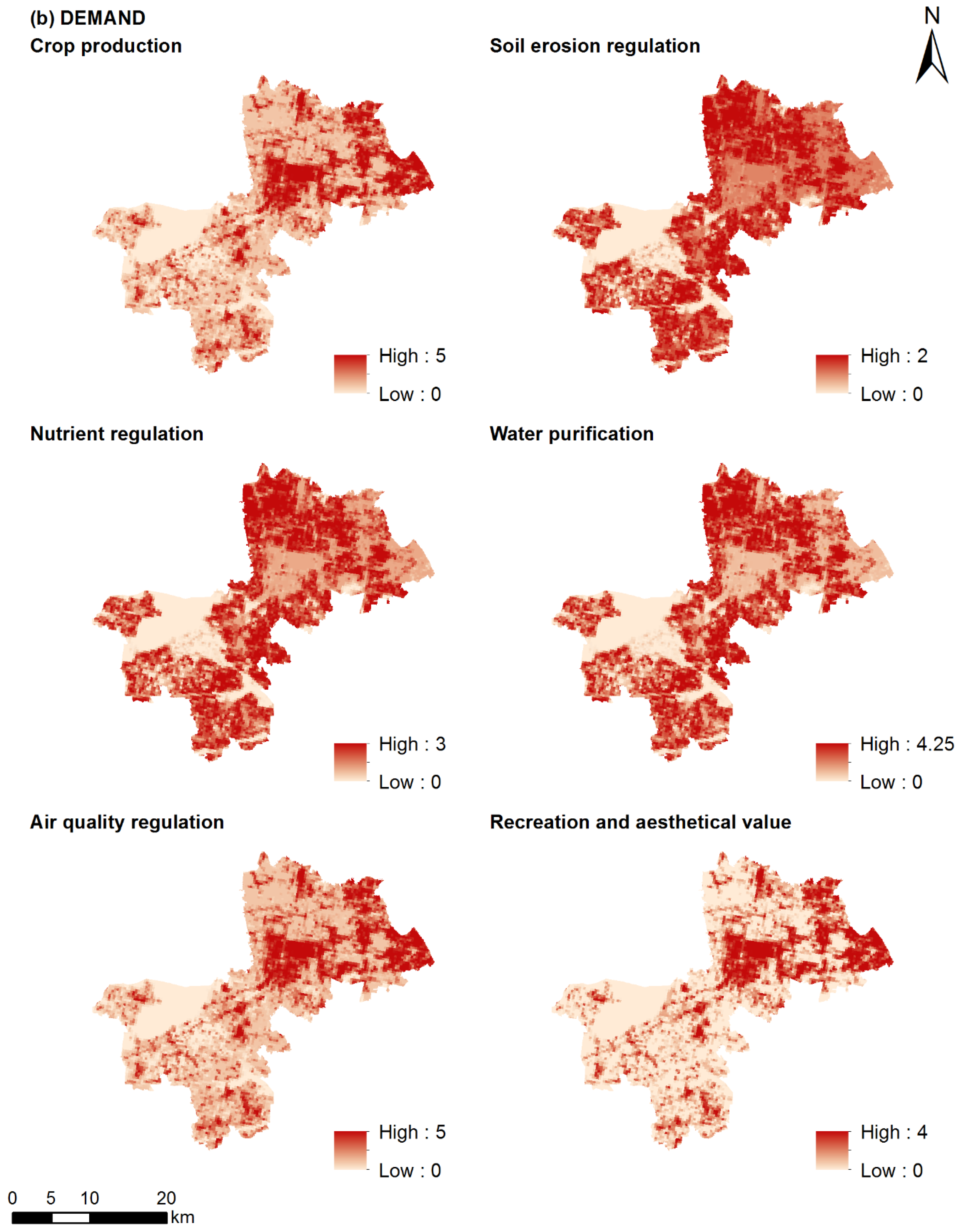
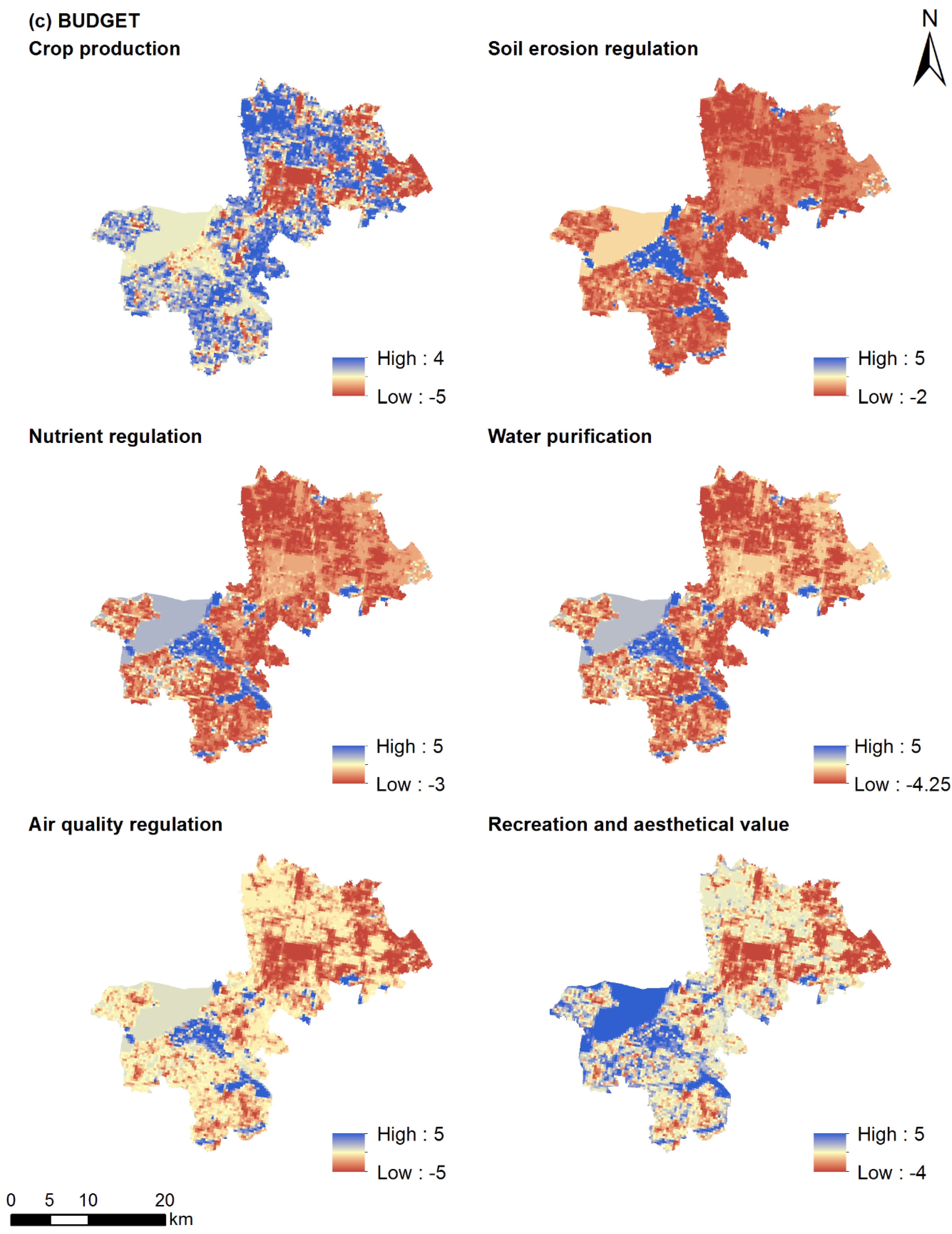
3.2. Spatial Distribution of Landscape Services in 2015

Figure 3 demonstrates the spatial distribution of the supply, demand, and budget of the six landscape services, which were characterized by pronounced spatial heterogeneity in 2015. Generally, the landscape service supply was higher on the west wing than that on the east wing. The supply of the four ecological services followed a similar spatial pattern, whereby an abundant supply of nutrient regulation, air-quality regulation, soil-erosion regulation, and water purification was observed in the forest located on the southeast side of Dianshan Lake. Crop production was provided relatively equally across Qingpu, except that lower values existed in the waters, the center of Qingpu, and the regions close to Shanghai central city. Recreation and aesthetical value was mainly produced by the west wing on account of the biophysical context; however, the difference between the east and the west was not as striking as the ecological services.

Demand for landscape services exhibited quite different characteristics from the supply, whereby higher values were mainly located in the east than in the west. Spatial consistency existed in the pair of crop production and air-quality regulation because of the demand matrix. Crop production, air-quality regulation, and recreation and aesthetical value were required the most in the urban area of Qingpu and the regions close to central Shanghai, whereas the regions with a large amount of arable land represented a higher demand for nutrient regulation, soil-erosion regulation, and water purification.

The imbalance of supply and demand of landscape services was extensively observed in Qingpu. Budget surpluses of landscape services, except for crop production, were observed mainly in the west wing, especially Dianshan Lake and its surrounding forest. High-value regions of crop production budget could be found mainly to the west and north of Qingpu. Budget deficits of nutrient regulation, soil-erosion regulation, and water purification covered a large area across Qingpu. In addition, the budgets of crop production, air-quality regulation, and recreation and aesthetical value were particularly tight in the center of Qingpu and the region adjacent to central Shanghai.

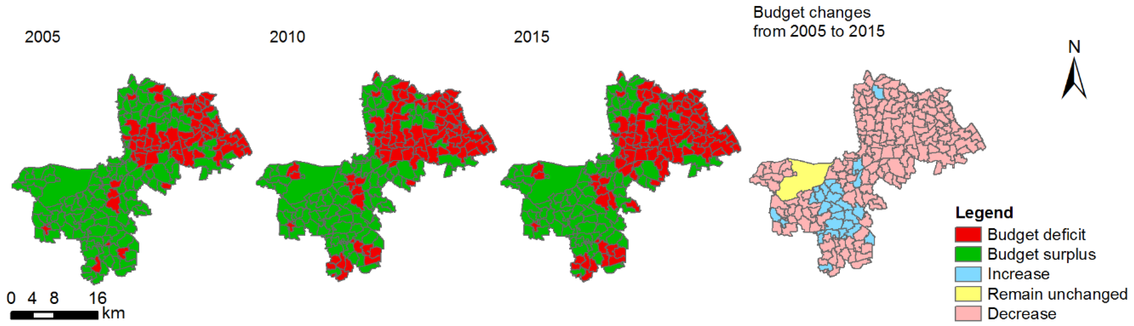
3.3. Spatiotemporal Variations of Landscape Multifunctionality Budget

The results of spatiotemporal variations of landscape multifunctionality budget are presented at the village level in Figure 4. There was an obvious difference in B_MFI between the east and the west wing. Villages with deficits of B_MFI gathered on the east wing, whereas budget surplus existed mainly on the west wing. During the decade, the regions with limited budget expanded continuously as the percentage of villages suffering from the budget deficit of landscape multifunctionality in 2005, 2010, and 2015 was 32%, 45%, and 50%, respectively. The landscape multifunctionality budget shrank in 85% of villages in the ten years, while improvement could be observed mostly around Dianshan Lake.

Table 4. Global Moran’s I (p < 0.001) values and their Z-scores of landscape multifunctionality budget index (B_MFI).

Year	2005	2010	2015
Moran’s I	0.5410	0.5952	0.6335
Z-score	12.4286	13.2448	13.8583

illustrates the spatial agglomeration of B_MFI in Qingpu. Gradually increasing Moran’s I scores and Z-scores revealed that the spatial agglomeration of landscape multifunctionality was constantly enhanced from 2005 to 2015, that is to say, the differentiation between the east wing and the west wing became more obvious. The hot and cold spots of the landscape multifunctionality budget in 2015 are shown in Figure 5. Dianshan Lake and its neighboring villages covered by dense forest were regarded as hotspots, and unsurprisingly, cold spots of villages were observed in the center of Qingpu and near Shanghai central city.

3.4. Influencing Factors Associated with Landscape Multifunctionality Budget

Table 5. Results of the linear regression analysis.

Explanatory Variables	Coefficient	t-Value	p-Value	Tolerance	VIF
Constant	−1.0958	−5.3911	0.0000
ED	−0.6410	−1.2786	0.2025	0.1672	5.9797
SHDI	1.0847 *	2.0155	0.0451	0.1451	6.8929
CONTAG	0.5528 *	2.4571	0.0149	0.8303	1.2044
PopDen	−0.9615 **	−4.3066	0.0000	0.8431	1.1862
DisSH	1.0477 **	2.6453	0.0088	0.2679	3.7330
DisQP	−0.2980	−0.9825	0.3078	0.4887	2.0463
AI	−0.9510 **	−3.5220	0.0006	0.5764	1.7348
ALA	0.0421	0.1080	0.9141	0.2824	3.5414
LF	−0.2312	−0.9554	0.3406	0.8743	1.1437
Edu	−0.4811	−1.5490	0.1231	0.4357	2.2954
R2	0.5052
Adjusted R2	0.4791
F	19.3964
Sig.	0.0000

See Table 2 for the definition of explanatory variables. * p < 0.05; ** p < 0.01.

shows the regression results. The tolerance values and variance inflation factors (VIFs) indicated the absence of multi-collinearity among the explanatory variables. F (19.3964) and Sig. (0.0000) reflect the statistical significance and reasonability of this regression. There were significant relationships between B_MFI and two landscape metrics and three socioeconomic indicators.

Shannon’s diversity index (SHDI) reflects the landscape structure to show the diversity and proportion of landscape units. Contagion index (CONTAG) measures the landscape textures to indicate the tendency of patch types being spatially aggregated [76]. These two indicators were prominently positively associated with B_MFI. SHDI had a strong impact on the landscape multifunctionality budget, but the role of CONTAG was more trivial than other explanatory variables. B_MFI showed an evident decreasing trend as population density and per capita annual income increased (negative relationships), indicating that multifunctionality budget decreased in villages with higher values for these two socioeconomic factors. Distance to the center of Shanghai had a significantly positive effect on B_MFI, that is to say, the closer to the city center of Shanghai, the more negative the landscape multifunctionality budget.

4. Discussion

4.1. Understanding Landscape Service Budget

Landscape service budget represents the excess supply–demand that remains in each part of the landscape after the potential service supply meets the maximum possible potential demand that it can reach [77]. The landscape multifunctionality budget comprehensively evaluates the supply–demand excess of the combination of the functions or services that landscapes can offer. By analyzing the status of budget surplus or deficit, we can clearly understand the complex relationship between human and environment, which, to some extent, reflects landscape sustainability [2,78].

The results showed that there were significant spatial and temporal variations of landscape service budget in Qingpu due to land cover and the underlying socio-ecological conditions. The temporal variations in Qingpu (Table 3) demonstrated that the budget of ecological services except air-quality regulation improved, which can be attributed to the substantial increase in forest area near Dianshan Lake and the decrease in arable land. Forest landscapes are acknowledged as the key landscape type for ecological sustainability [56]. Urban sprawl mainly proceeded via the occupation of arable land in the studied decade with arable land area dwindling by 22%. In spite of the improvement, the budgets of ecological services were still in deficit status, which was caused by heavy urban sprawl with built-up area increasing from about 119 km² in 2005 to 198 km² in 2015. The rising population pressures led to the high demand for multiple landscape services and decreased the budget.

Furthermore, the results showed that there were significant east–west differentiations of landscape multifunctionality budget, whereby hotspots aggregated in the west wing and cold spots gathered in the center and the east wing near central Shanghai. In the east wing, the adjacency to central Shanghai is conducive to rapid urban sprawl and land-use change. Much arable land was converted to built-up areas around the existing urbanized area, resulting in the convenience of transportation and infrastructure, the development of economics, the attraction of population, and a higher income than that engaged in agriculture in rural area. Meanwhile, the landscape patterns in these urban fringes became more fragmented and less diverse because of the staggered distribution of multiple land uses. Thus, these densely populated regions represent high levels of human activities, where a high budget deficit, as well as a low diversity of landscape services, preponderate. The west wing of Qingpu is dominated by a larger proportion of natural landscapes with low-intensity human activities, exhibiting diverse landscape units and aggregated landscape patterns, generating a high multifunctionality budget. However, the population density and average income were relatively low in these regions.

The landscape multifunctionality budget, as a comprehensive index integrating the supply–demand relationships of multiple landscape services, can be very useful for decision-makers and local stakeholders for the spatial and temporal comparison of landscape service status in suburban regions. Identifying the budget surplus or deficit status can help assess the dependence of a region on landscape services or its potential for exporting certain goods and services. Quantification of the service budget is essential for making the best possible use of available potential landscape service supply in meeting the needs of various possible beneficiaries across the landscape [77] for the better development of suburban areas.

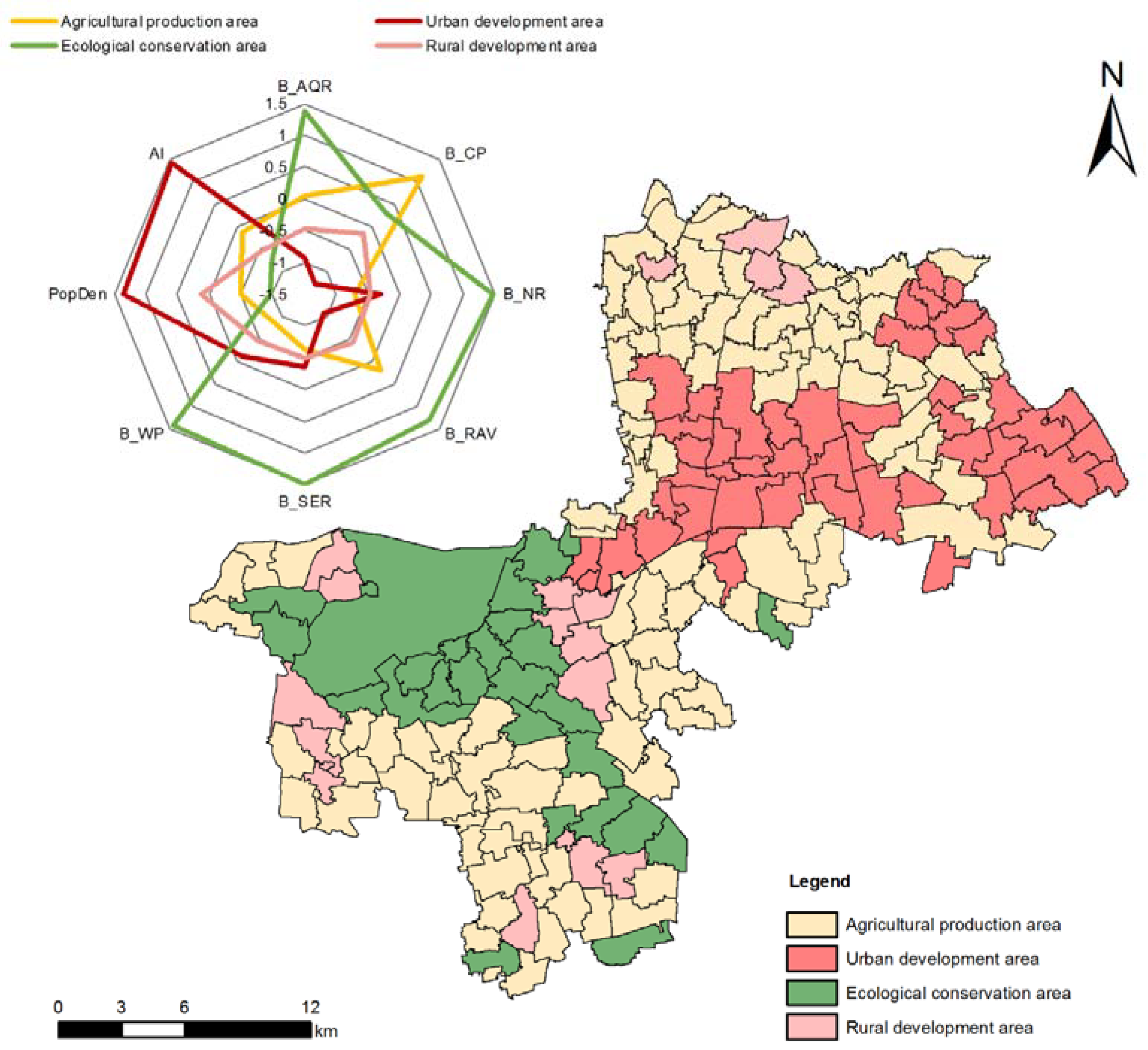
4.2. Landscape Function Zoning and Policy Implications

The development of a district is of great relevance in the biophysical and socioeconomic context; thus, optimal landscape stewardship should be launched in light of local circumstances with the joint consideration of all the objectives. Landscape function zoning was conducted via cluster analysis based on the budget of six landscape services, the population density, and the per capita annual income of each village. Villages of Qingpu (including Dianshan Lake) were divided into four functional zones: urban development area, rural development area, agricultural production area, and ecological conservation area (Figure 6).

The urban development area is mainly located on the east wing near central Shanghai and the center of Qingpu, which are cold spots of the landscape multifunctionality budget. Overall mismatches of landscape services exist in this area, whereby the supply cannot meet the demand of the large population in these villages. Meanwhile, this area is the most economically developed area in Qingpu with the highest urbanization level and average income. The center of Qingpu is the political and cultural center where the district government and administrative departments are situated, and the east wing under the economic radiation of Shanghai central city contributes greatly to the improvement of the socioeconomic competitiveness of Qingpu. With workers commuting to central Shanghai every day, the urban development area also relieves the population pressure of Shanghai central city. The regional superiority offers the urban development area advantages to promote the secondary and tertiary industry. Transportation, education, medicine, and other public services and infrastructures should be enhanced. However, urban construction relies much on land inputs which decrease landscape services; therefore, it is urgent to negotiate the relationship between urban development and ecological protection, and to accelerate the industrial upgrading to achieve environmentally friendly and resource-saving development. Promoting built-up land use more efficiently and intensively will be a good strategy, and urban green design should gain more attention.

The agricultural production area is widely distributed in Qingpu, mainly in the west and north parts (Liantang, Zhujiajiao, and Baihe). Preserving arable land in suburbs plays an important role in guaranteeing food security [79] for the sustained growth of population of Qingpu and even Shanghai. Maintaining the agricultural landscape’s sustainability in suburban areas is a priority [80]. Effective measures should be taken to prevent agricultural pollution and maintain soil quality, such as the limitation of the use of fertilizer and pesticides and the enlargement of the utilization of green manure. Additionally, farmland transfer policy applied in this area proved to be effective in improving the living conditions of rural households [81]. Professional farmers rent farmland from others to realize the appropriate scale of management and engage their labor forces in farming activities, while laborers of other households can be involved in off-farm employment.

The ecological conservation area covers Dianshan Lake and neighboring villages dominated by forest. This area comprises hotspots of the landscape multifunctionality budget and shows by far the strongest function of air-quality regulation, nutrient regulation, soil-erosion regulation, water purification, and recreation and aesthetical value; however, the living standard in these villages is relatively low. Conservation of the forest and waters is directly related to the sustainability of Qingpu and it is crucial to improve the awareness of stakeholders. Dianshan Lake is one of the main drinking water sources for the huge population in Shanghai; thus, it is a matter of vital importance that it be protected. Low-impact eco-tourism should be encouraged to meet the huge increasing demand of recreation and leisure activities of urban dwellers. In this area, the proportion of non-ecological land use should be restricted, and ecological land protection policies in China, such as setting the “ecological control line” [82] should also be implemented, coupled with sustainable utilization and management of natural capitals, resulting in a win–win development in terms of the ecology and economy. Meanwhile, the establishment of eco-compensation mechanisms is also an urgent task to balance the interests of stakeholders.

The rural development area covers the center villages of Jinze, Liantang, and Zhujiajiao on the west wing and Baihe in the north of Qingpu. These villages have slightly higher landscape service supply than the urban developing area, and moderate demand. The rural development area provides residential space for rural inhabitants; however, the average income is relatively low. Public infrastructures should be constructed to improve the living conditions and convenience of rural residents. For the west wing, these villages can take advantage of the adjacency to Dianshan Lake to develop eco-resorts, as people prefer to travel to more natural habitats that surround areas of water [83]. The restriction of the expansion scale of built-up areas should be an essential management task in this region; therefore, large-scale construction and industry with high-level environment pollution should be controlled.

4.3. Limitations, Uncertainties, and Contributions of the Research

Our research applied an effective framework for assessing landscape services and developed B_MFI to conduct further analysis identifying the hot and cold spots and influencing factors, and informed landscape function zoning strategies. However, there are still limitations and uncertainties in this study. Firstly, although the supply and demand matrices were adjusted according to the local situation, the framework cannot completely avoid the subjectivity of an expert scoring method. The supply and demand are reflected by spatially explicit data instead of primary data due to the limitation of data accessibility. On the one hand, the same land-cover type may have different capacity to supply landscape services. For example, some of the natural forests were changed to artificial forests for years and it is likely that the services provided by artificial forests are much lower than those by natural forests [66]. On the other hand, the demand for landscape services is not calculated based on the stakeholder survey [74] or participatory mapping techniques [84]. Secondly, for the selection of landscape services, this study mainly consists of the six representative services, but cannot reflect all the landscape services, and ignored services such as residential space will be evaluated in the future. Additionally, different weights of landscape service for calculating the multifunctionality will also generate uncertainties in the results.

Despite the limitations and uncertainties, there are still some contributions. This paper presented a comprehensive index called the landscape multifunctionality budget (B_MFI), enabled the direct comparison of multiple landscape service supplies and demands, and innovatively integrated the concept of budget surplus and deficit with multiple landscape services. As a representative suburban area in Shanghai metropolis, the typical role of Qingpu in suburban development has some reference value for the agricultural and socioeconomic development of many regions in the context of rapid urbanization. However, researches taking Qingpu as a case study area are rather rare [81,85]. This paper enriches the existing research about landscape services in suburban regions, synthesizes hotspots and influencing factor identification into the landscape multifunctionality budget, and further informs landscape function zoning at the village level, coordinating economy and ecology. For other data-scarce suburban regions like Qingpu in an international context, the semi-quantitative assessment of landscape services using expert knowledge combined with the local situation can be applied because of its dimensionless format [33], and it is easier to obtain than observed results by fieldwork. This framework could simplify the complexity involved in the diagnosis of landscape service supply–demand mismatches and the identification of spatial agglomeration and influencing factors in the rapid urbanization process, providing valuable information and laying the foundation for further researches.

5. Conclusions

This paper applied a comprehensive framework for assessing and mapping the temporal and spatial variations of landscape service supply, demand, and budget, and conducted further analysis from the integrative perspective of the landscape multifunctionality budget for the identification of hot and cold spots, and influencing factors. This paper preliminarily identified the surplus and deficit of landscape services and landscape multifunctionlity, supporting further research and providing an orientation for landscape management. We demonstrated that the supply and demand matrices proposed by Burkhard et al. [38] are effective for assessing landscape services in a suburban area, and that the landscape multifunctionality budget is a useful tool for aggregating multiple landscape service supplies and demands. The results indicate that land-cover change and the underlying socioeconomic conditions caused by rapid urban sprawl are the main drivers of the temporal and spatial variations of landscape services and landscape multifunctionality budget. During the decade, the rapid expansion of built-up areas proceeded with the decrement of arable land, while forest area increased near Dianshan Lake. Consequently, ecological services except air-quality regulation performed better in 2015 at the cost of crop production, and the recreation and aesthetical value weakened. Landscape service budgets generally follow the spatial pattern of positive in the west and negative in the east. The budget deficit of nutrient regulation, soil-erosion regulation, and water purification was widely distributed across Qingpu. The landscape multifunctionality budget of Qingpu was in surplus status in 2005 and 2010, but turned to deficit status in 2015 due to urban expansion. Budget deficit covered half of the villages in 2015, which were mainly situated in the east wing. Villages near central Shanghai, on the one hand, can benefit from urbanization to improve average income; however, on the other hand, they cope with population pressure and suffer from fragmented and less diverse landscape patterns, resulting in a negative trend in the landscape multifunctional budget.

Suburban areas like Qingpu District, due to specific location, are often an arena of complex and sometimes contradicting demands and are increasingly demanding multifunctional landscape. Qingpu is coping and will increasingly have to cope with population growth. In this urbanizing process, considering regional conditions, the imbalance between the west wing and the east wing can also be regarded as a harmonious status from a holistic perspective. According to the budget status of surplus and deficit, city planners and policy-makers should focus on ecological conservation in the west wing and economic development in the east wing, taking advantage of the neighboring Shanghai central city. We suggest context-specific landscape function zoning as an effective way to achieve the win–win development of ecology and economics and to improve the comprehensive competitiveness of Qingpu achieving a sustainable future. The research still calls for improvements, such as quantitative modeling of landscape service supply, and the detailed calculation of landscape service demand, which will be conducted in future work. Moreover, scenario analysis with the land-use model will be applied to explore alternative land-use patterns for optimal landscape services and higher landscape multifunctionality budgets, further supporting practical landscape planning.

References

1. Bastian, O.; Grunewald, K.; Syrbe, R.-U.; Walz, U.; Wende, W. Landscape services: The concept and its practical relevance. Landsc. Ecol. 2014, 29, 1463–1479. [Google Scholar] [CrossRef]
2. Fang, X.; Zhao, W.; Fu, B.; Ding, J. Landscape service capability, landscape service flow and landscape service demand: A new framework for landscape services and its use for landscape sustainability assessment. Prog. Phys. Geogr. 2015, 39, 817–836. [Google Scholar] [CrossRef]
3. Pfeifer, C.; Sonneveld, M.P.; Stoorvogel, J.J. Farmers’ contribution to landscape services in the Netherlands under different rural development scenarios. J. Environ. Manag. 2012, 111, 96–105. [Google Scholar] [CrossRef] [PubMed]
4. Termorshuizen, J.W.; Opdam, P. Landscape services as a bridge between landscape ecology and sustainable development. Landsc. Ecol. 2009, 24, 1037–1052. [Google Scholar] [CrossRef]
5. Gulickx, M.M.C.; Verburg, P.H.; Stoorvogel, J.J.; Kok, K.; Veldkamp, A. Mapping landscape services: A case study in a multifunctional rural landscape in The Netherlands. Ecol. Indic. 2013, 24, 273–283. [Google Scholar] [CrossRef]
6. Ungaro, F.; Zasada, I.; Piorr, A. Mapping landscape services, spatial synergies and trade-offs. A case study using variogram models and geostatistical simulations in an agrarian landscape in North-East Germany. Ecol. Indic. 2014, 46, 367–378. [Google Scholar] [CrossRef]
7. Aretano, R.; Petrosillo, I.; Zaccarelli, N.; Semeraro, T.; Zurlini, G. People perception of landscape change effects on ecosystem services in small Mediterranean islands: A combination of subjective and objective assessments. Landsc. Urban Plan. 2013, 112, 63–73. [Google Scholar] [CrossRef]
8. De Groot, R.S.; Alkemade, R.; Braat, L.; Hein, L.; Willemen, L. Challenges in integrating the concept of ecosystem services and values in landscape planning, management and decision making. Ecol. Complex. 2010, 7, 260–272. [Google Scholar] [CrossRef]
9. Estoque, R.C.; Murayama, Y. Landscape pattern and ecosystem service value changes: Implications for environmental sustainability planning for the rapidly urbanizing summer capital of the Philippines. Landsc. Urban Plan. 2013, 116, 60–72. [Google Scholar] [CrossRef]
10. Jackson, B.; Pagella, T.; Sinclair, F.; Orellana, B.; Henshaw, A.; Reynolds, B.; McIntyre, N.; Wheater, H.; Eycott, A. Polyscape: A GIS mapping framework providing efficient and spatially explicit landscape-scale valuation of multiple ecosystem services. Landsc. Urban Plan. 2013, 112, 74–88. [Google Scholar] [CrossRef]
11. Lamarque, P.; Quetier, F.; Lavorel, S. The diversity of the ecosystem services concept and its implications for their assessment and management. C. R. Biol. 2011, 334, 441–449. [Google Scholar] [CrossRef] [PubMed]
12. Musacchio, L.R. Cultivating deep care: Integrating landscape ecological research into the cultural dimension of ecosystem services. Landsc. Ecol. 2013, 28, 1025–1038. [Google Scholar] [CrossRef]
13. Syrbe, R.-U.; Walz, U. Spatial indicators for the assessment of ecosystem services: Providing, benefiting and connecting areas and landscape metrics. Ecol. Indic. 2012, 21, 80–88. [Google Scholar] [CrossRef]
14. Hermann, A.; Kuttner, M.; Hainz-Renetzeder, C.; Konkoly-Gyuró, É.; Tirászi, Á.; Brandenburg, C.; Allex, B.; Ziener, K.; Wrbka, T. Assessment framework for landscape services in European cultural landscapes: An Austrian Hungarian case study. Ecol. Indic. 2014, 37, 229–240. [Google Scholar] [CrossRef]
15. Peng, J.; Liu, Y.; Liu, Z.; Yang, Y. Mapping spatial non-stationarity of human-natural factors associated with agricultural landscape multifunctionality in Beijing–Tianjin–Hebei region, China. Agric. Ecosyst. Environ. 2017, 246, 221–233. [Google Scholar] [CrossRef]
16. Fagerholm, N.; Käyhkö, N.; Ndumbaro, F.; Khamis, M. Community stakeholders’ knowledge in landscape assessments—Mapping indicators for landscape services. Ecol. Indic. 2012, 18, 421–433. [Google Scholar] [CrossRef]
17. Wu, J.; Feng, Z.; Gao, Y.; Peng, J. Hotspot and relationship identification in multiple landscape services: A case study on an area with intensive human activities. Ecol. Indic. 2013, 29, 529–537. [Google Scholar] [CrossRef]
18. Willemen, L.; Veldkamp, A.; Verburg, P.H.; Hein, L.; Leemans, R. A multi-scale modelling approach for analysing landscape service dynamics. J. Environ. Manag. 2012, 100, 86–95. [Google Scholar] [CrossRef] [PubMed]
19. Bolliger, J.; Bättig, M.; Gallati, J.; Kläy, A.; Stauffacher, M.; Kienast, F. Landscape multifunctionality: A powerful concept to identify effects of environmental change. Reg. Environ. Chang. 2010, 11, 203–206. [Google Scholar] [CrossRef]
20. Wu, J. Landscape sustainability science: Ecosystem services and human well-being in changing landscapes. Landsc. Ecol. 2013, 28, 999–1023. [Google Scholar] [CrossRef]
21. Gimona, A.; van der Horst, D. Mapping hotspots of multiple landscape functions: A case study on farmland afforestation in Scotland. Landsc. Ecol. 2007, 22, 1255–1264. [Google Scholar] [CrossRef]
22. Li, J.; Jiang, H.; Bai, Y.; Alatalo, J.M.; Li, X.; Jiang, H.; Liu, G.; Xu, J. Indicators for spatial–temporal comparisons of ecosystem service status between regions: A case study of the Taihu River Basin, China. Ecol. Indic. 2016, 60, 1008–1016. [Google Scholar] [CrossRef]
23. Sun, X.; Crittenden, J.C.; Li, F.; Lu, Z.; Dou, X. Urban expansion simulation and the spatio-temporal changes of ecosystem services, a case study in Atlanta Metropolitan area, USA. Sci. Total Environ. 2018, 622–623, 974–987. [Google Scholar] [CrossRef] [PubMed]
24. Willemen, L.; Hein, L.; Verburg, P.H. Evaluating the impact of regional development policies on future landscape services. Ecol. Econ. 2010, 69, 2244–2254. [Google Scholar] [CrossRef]
25. Braat, L.C.; de Groot, R. The ecosystem services agenda:bridging the worlds of natural science and economics, conservation and development, and public and private policy. Ecosyst. Serv. 2012, 1, 4–15. [Google Scholar] [CrossRef]
26. Ridding, L.E.; Redhead, J.W.; Oliver, T.H.; Schmucki, R.; McGinlay, J.; Graves, A.R.; Morris, J.; Bradbury, R.B.; King, H.; Bullock, J.M. The importance of landscape characteristics for the delivery of cultural ecosystem services. J. Environ. Manag. 2018, 206, 1145–1154. [Google Scholar] [CrossRef] [PubMed]
27. Tallis, H.; Kareiva, P.; Marvier, M.; Chang, A. An ecosystem services framework to support both practical conservation and economic development. Proc. Natl. Acad. Sci. USA 2008, 105, 9457–9464. [Google Scholar] [CrossRef] [PubMed] [Green Version]
28. Maes, J.; Egoh, B.; Willemen, L.; Liquete, C.; Vihervaara, P.; Schägner, J.P.; Grizzetti, B.; Drakou, E.G.; Notte, A.L.; Zulian, G.; et al. Mapping ecosystem services for policy support and decision making in the European Union. Ecosyst. Serv. 2012, 1, 31–39. [Google Scholar] [CrossRef]
29. Sun, X.; Li, F. Spatiotemporal assessment and trade-offs of multiple ecosystem services based on land use changes in Zengcheng, China. Sci. Total Environ. 2017, 609, 1569–1581. [Google Scholar] [CrossRef] [PubMed]
30. Vihervaara, P.; Mononen, L.; Santos, F.; Adamescu, M.; Cazacu, C.; Luque, S.; Geneletti, D.; Maes, J. Ecosystem services quantification. In Mapping Ecosystem Services, 1st ed.; Burkhard, B., Maes, J., Eds.; Pensoft Publishers: Sofia, Bulgaria, 2017; Volume 1, pp. 91–146. [Google Scholar]
31. Hu, Y.; Peng, J.; Liu, Y.; Tian, L. Integrating ecosystem services trade-offs with paddy land-to-dry land decisions: A scenario approach in Erhai Lake Basin, southwest China. Sci. Total Environ. 2018, 625, 849–860. [Google Scholar] [CrossRef] [PubMed]
32. Wang, J.; Peng, J.; Zhao, M.; Liu, Y.; Chen, Y. Significant trade-off for the impact of Grain-for-Green Programme on ecosystem services in North-western Yunnan, China. Sci. Total Environ. 2017, 574, 57–64. [Google Scholar] [CrossRef] [PubMed]
33. García-Ayllón, S. Predictive Diagnosis of Agricultural Periurban Areas Based on Territorial Indicators: Comparative Landscape Trends of the So-Called “Orchard of Europe”. Sustainability 2018, 10, 1820. [Google Scholar] [CrossRef]
34. Costanza, R.; d’Arge, R.; de Groot, R.; Farber, S.; Grasso, M.; Hannon, B.; Limburg, K.; Naeem, S.; O’Neill, R.V.; Paruelo, J.; et al. The value of the world’s ecosystem services and natural capital. Nature 1997, 387, 253–260. [Google Scholar] [CrossRef]
35. Goldstein, J.H.; Caldarone, G.; Duarte, T.K.; Ennaanay, D.; Hannahs, N.; Mendoza, G.; Polasky, S.; Wolny, S.; Daily, G.C. Integrating ecosystem-service tradeoffs into land-use decisions. Proc. Natl. Acad. Sci. USA 2012, 109, 7565–7570. [Google Scholar] [CrossRef] [PubMed] [Green Version]
36. Xie, G.; Zhang, C.; Zhen, L.; Zhang, L. Dynamic changes in the value of China’s ecosystem services. Ecosyst. Serv. 2017, 26, 146–154. [Google Scholar] [CrossRef]
37. Burkhard, B.; Kroll, F.; Müller, F. Landscapes‘ Capacities to Provide Ecosystem Services—A Concept for Land-Cover Based Assessments. Landsc. Online 2009, 15, 1–22. [Google Scholar] [CrossRef]
38. Burkhard, B.; Kroll, F.; Nedkov, S.; Müller, F. Mapping ecosystem service supply, demand and budgets. Ecol. Indic. 2012, 21, 17–29. [Google Scholar] [CrossRef]
39. Spangenberg, J.H.; Settele, J. Precisely incorrect? Monetising the value of ecosystem services. Ecol. Complex. 2010, 7, 327–337. [Google Scholar] [CrossRef]
40. Veldkamp, A.; Verburg, P.H. Modelling land use change and environmental impact. J. Environ. Manag. 2004, 72, 1–3. [Google Scholar] [CrossRef] [PubMed]
41. Veldkamp, P.H.; Schot, P.P.; Dijst, M.J.; Veldkamp, D.A. Land use change modelling: Current practice and research priorities. GeoJournal 2004, 61, 309–324. [Google Scholar] [CrossRef]
42. Salata, S. Land use change analysis in the urban region of Milan. Manag. Environ. Qual. Int. J. 2017, 28, 879–901. [Google Scholar] [CrossRef]
43. Benini, L.; Bandini, V.; Marazza, D.; Contin, A. Assessment of land use changes through an indicator-based approach: A case study from the Lamone river basin in Northern Italy. Ecol. Indic. 2010, 10, 4–14. [Google Scholar] [CrossRef]
44. Baró, F.; Gómez-Baggethun, E.; Haase, D. Ecosystem service bundles along the urban-rural gradient: Insights for landscape planning and management. Ecosyst. Serv. 2017, 24, 147–159. [Google Scholar] [CrossRef]
45. Chen, Y.; Yu, Z.; Li, X.; Li, P. How agricultural multiple ecosystem services respond to socioeconomic factors in Mengyin County, China. Sci. Total Environ. 2018, 630, 1003–1015. [Google Scholar] [CrossRef] [PubMed]
46. Bryan, B.A.; Raymond, C.M.; Crossman, N.D.; Macdonald, D.H. Targeting the management of ecosystem services based on social values: Where, what, and how? Landsc. Urban Plan. 2010, 97, 111–122. [Google Scholar] [CrossRef]
47. Burkhard, B.; Kandziora, M.; Hou, Y.; Müller, F. Ecosystem Service Potentials, Flows and Demands – Concepts for Spatial Localisation, Indication and Quantification. Landsc. Online 2014, 34, 1–32. [Google Scholar] [CrossRef]
48. Muhamad, D.; Okubo, S.; Harashina, K.; Parikesit; Gunawan, B.; Takeuchi, K. Living close to forests enhances people’s perception of ecosystem services in a forest–agricultural landscape of West Java, Indonesia. Ecosyst. Serv. 2014, 8, 197–206. [Google Scholar] [CrossRef]
49. Van Jaarsveld, A.S.; Biggs, R.; Scholes, R.J.; Bohensky, E.; Reyers, B.; Lynam, T.; Musvoto, C.; Fabricius, C. Measuring conditions and trends in ecosystem services at multiple scales: The Southern African Millennium Ecosystem Assessment (SAfMA) experience. Philos. Trans. R. Soc. B-Biol. Sci. 2005, 360, 425–441. [Google Scholar] [CrossRef] [PubMed]
50. Westerink, J.; Opdam, P.; van Rooij, S.; Steingröver, E. Landscape services as boundary concept in landscape governance: Building social capital in collaboration and adapting the landscape. Land Use Policy 2017, 60, 408–418. [Google Scholar] [CrossRef]
51. Honey-Rosés, J.; Acuña, V.; Bardina, M.; Brozović, N.; Marcé, R.; Munné, A.; Sabater, S.; Termes, M.; Valero, F.; Vega, À.; et al. Examining the Demand for Ecosystem Services: The Value of Stream Restoration for Drinking Water Treatment Managers in the Llobregat River, Spain. Ecol. Econ. 2013, 90, 196–205. [Google Scholar] [CrossRef]
52. Orenstein, D.E.; Groner, E. In the eye of the stakeholder: Changes in perceptions of ecosystem services across an international border. Ecosyst. Serv. 2014, 8, 185–196. [Google Scholar] [CrossRef]
53. Wolff, S.; Schulp, C.J.E.; Verburg, P.H. Mapping ecosystem services demand: A review of current research and future perspectives. Ecol. Indic. 2015, 55, 159–171. [Google Scholar] [CrossRef]
54. Wolff, S.; Schulp, C.J.E.; Kastner, T.; Verburg, P.H. Quantifying Spatial Variation in Ecosystem Services Demand: A Global Mapping Approach. Ecol. Econ. 2017, 136, 14–29. [Google Scholar] [CrossRef]
55. Burkhard, B.; Maes, J. Introduction. In Mapping Ecosystem Services, 1st ed.; Burkhard, B., Maes, J., Eds.; Pensoft Publishers: Sofia, Bulgaria, 2017; Volume 1, pp. 25–27. [Google Scholar]
56. Peng, J.; Chen, X.; Liu, Y.; Lü, H.; Hu, X. Spatial identification of multifunctional landscapes and associated influencing factors in the Beijing-Tianjin-Hebei region, China. Appl. Geogr. 2016, 74, 170–181. [Google Scholar] [CrossRef]
57. Rodríguez-Loinaz, G.; Alday, J.G.; Onaindia, M. Multiple ecosystem services landscape index: A tool for multifunctional landscapes conservation. J. Environ. Manag. 2015, 147, 152–163. [Google Scholar] [CrossRef] [PubMed]
58. Zhang, Z.; Gao, J.; Fan, X.; Lan, Y.; Zhao, M. Response of ecosystem services to socioeconomic development in the Yangtze River Basin, China. Ecol. Indic. 2017, 72, 481–493. [Google Scholar] [CrossRef]
59. Peng, J.; Liu, Z.; Liu, Y.; Hu, X.; Wang, A. Multifunctionality assessment of urban agriculture in Beijing City, China. Sci. Total Environ. 2015, 537, 343–351. [Google Scholar] [CrossRef] [PubMed]
60. Gao, Y.; Feng, Z.; Li, Y.; Li, S. Freshwater ecosystem service footprint model: A model to evaluate regional freshwater sustainable development—A case study in Beijing–Tianjin–Hebei, China. Ecol. Indic. 2014, 39, 1–9. [Google Scholar] [CrossRef]
61. Su, S.; Xiao, R.; Jiang, Z.; Zhang, Y. Characterizing landscape pattern and ecosystem service value changes for urbanization impacts at an eco-regional scale. Appl. Geogr. 2012, 34, 295–305. [Google Scholar] [CrossRef]
62. Dai, E.; Wang, Y.; Ma, L.; Yin, L.; Wu, Z. ‘Urban-Rural’ Gradient Analysis of Landscape Changes around Cities in Mountainous Regions: A Case Study of the Hengduan Mountain Region in Southwest China. Sustainability 2018, 10, 1019. [Google Scholar] [CrossRef]
63. Zasada, I. Multifunctional peri-urban agriculture—A review of societal demands and the provision of goods and services by farming. Land Use Policy 2011, 28, 639–648. [Google Scholar] [CrossRef]
64. Früh-Müller, A.; Hotes, S.; Breuer, L.; Wolters, V.; Koellner, T. Regional Patterns of Ecosystem Services in Cultural Landscapes. Land 2016, 5, 17. [Google Scholar] [CrossRef]
65. Raudsepp-Hearne, C.; Peterson, G.D.; Bennett, E.M. Ecosystem service bundles for analyzing tradeoffs in diverse landscapes. Proc. Natl. Acad. Sci. USA. 2010, 107, 5242–5247. [Google Scholar] [CrossRef] [PubMed] [Green Version]
66. Cai, W.; Gibbs, D.; Zhang, L.; Ferrier, G.; Cai, Y. Identifying hotspots and management of critical ecosystem services in rapidly urbanizing Yangtze River Delta Region, China. J. Environ. Manag. 2017, 191, 258–267. [Google Scholar] [CrossRef] [PubMed]
67. Stoll, S.; Frenzel, M.; Burkhard, B.; Adamescu, M.; Augustaitis, A.; Baeßler, C.; Bonet, F.J.; Carranza, M.L.; Cazacu, C.; Cosor, G.L.; et al. Assessment of ecosystem integrity and service gradients across Europe using the LTER Europe network. Ecol. Model. 2015, 295, 75–87. [Google Scholar] [CrossRef]
68. Tao, Y.; Wang, H.; Ou, W.; Guo, J. A land-cover-based approach to assessing ecosystem services supply and demand dynamics in the rapidly urbanizing Yangtze River Delta region. Land Use Policy 2018, 72, 250–258. [Google Scholar] [CrossRef]
69. Qingpu Statistical Bureau. Qingpu Statistical Yearbook 2005; Qingpu Statistical Bureau: Shanghai, China, 2006.
70. Qingpu Statistical Bureau. Qingpu Statistical Yearbook 2015; Qingpu Statistical Bureau: Shanghai, China, 2016.
71. Shanghai Municipal Statistics Bureau. Shanghai Statistical Yearbook 2015; Shanghai Municipal Statistics Bureau: Shanghai, China, 2016.
72. Liu, J.; Kuang, W.; Zhang, Z.; Xu, X.; Qin, Y.; Ning, J.; Zhou, W.; Zhang, S.; Li, R.; Yan, C.; et al. Spatiotemporal characteristics, patterns, and causes of land-use changes in China since the late 1980s. J. Geogr. Sci. 2014, 24, 195–210. [Google Scholar] [CrossRef]
73. Geospatial Data Cloud. Available online: http://www.gscloud.cn/ (accessed on 4 January 2016).
74. Garcia-Ayllon, S. The Integrated Territorial Investment (ITI) of the Mar Menor as a model for the future in the comprehensive management of enclosed coastal seas. Ocean Coast. Manag. 2018. [Google Scholar] [CrossRef]
75. Anselin, L. Local Indicators of Spatial Association-LISA. Geogr. Anal. 1995, 27, 93–115. [Google Scholar] [CrossRef]
76. Feng, Y.; Liu, Y.; Tong, X. Spatiotemporal variation of landscape patterns and their spatial determinants in Shanghai, China. Ecol. Indic. 2018, 87, 22–32. [Google Scholar] [CrossRef]
77. Goldenberg, R.; Kalantari, Z.; Cvetkovic, V.; Mortberg, U.; Deal, B.; Destouni, G. Distinction, quantification and mapping of potential and realized supply-demand of flow-dependent ecosystem services. Sci. Total Environ. 2017, 593–594, 599–609. [Google Scholar] [CrossRef] [PubMed]
78. Potschin, M.; Haines-Young, R. Landscapes, sustainability and the place-based analysis of ecosystem services. Landsc. Ecol. 2012, 28, 1053–1065. [Google Scholar] [CrossRef]
79. Barthel, S.; Isendahl, C. Urban gardens, agriculture, and water management: Sources of resilience for long-term food security in cities. Ecol. Econ. 2013, 86, 224–234. [Google Scholar] [CrossRef]
80. Gullino, P.; Battisti, L.; Larcher, F. Linking Multifunctionality and Sustainability for Valuing Peri-Urban Farming: A Case Study in the Turin Metropolitan Area (Italy). Sustainability 2018, 10, 1625. [Google Scholar] [CrossRef]
81. Liu, Z.; Liu, L. Characteristics and driving factors of rural livelihood transition in the east coastal region of China: A case study of suburban Shanghai. J. Rural Stud. 2016, 43, 145–158. [Google Scholar] [CrossRef]
82. Hong, W.; Yang, C.; Chen, L.; Zhang, F.; Shen, S.; Guo, R. Ecological control line: A decade of exploration and an innovative path of ecological land management for megacities in China. J. Environ. Manag. 2017, 191, 116–125. [Google Scholar] [CrossRef] [PubMed]
83. Paracchini, M.L.; Zulian, G.; Kopperoinen, L.; Maes, J.; Schägner, J.P.; Termansen, M.; Zandersen, M.; Perez-Soba, M.; Scholefield, P.A.; Bidoglio, G. Mapping cultural ecosystem services: A framework to assess the potential for outdoor recreation across the EU. Ecol. Indic. 2014, 45, 371–385. [Google Scholar] [CrossRef] [Green Version]
84. Brown, G.; Fagerholm, N. Empirical PPGIS/PGIS mapping of ecosystem services: A review and evaluation. Ecosyst. Serv. 2015, 13, 119–133. [Google Scholar] [CrossRef]
85. Feng, Y.; Liu, Y.; Batty, M. Modeling urban growth with GIS based cellular automata and least squares SVM rules: A case study in Qingpu–Songjiang area of Shanghai, China. Stoch. Environ. Res. Risk Manag. 2015, 30, 1387–1400. [Google Scholar] [CrossRef]
Figure 1. Workflow of the study process derived from our own elaboration based on Peng [56].
Sustainability 10 03752 g001
Figure 2. Location of the study area.
Sustainability 10 03752 g002
Figure 3. The (a) supply, (b) demand, and (c) budget of the six landscape services of Qingpu in 2015.
Sustainability 10 03752 g003aSustainability 10 03752 g003bSustainability 10 03752 g003c
Figure 4. Landscape multifunctionality budget of villages in Qingpu and the changes from 2005 to 2015.
Sustainability 10 03752 g004
Figure 5. Local Moran’s I cluster map of the landscape multifunctionality budget of Qingpu in 2015.
Sustainability 10 03752 g005
Figure 6. Landscape function zoning at the village level in Qingpu. The diagram shows average values of each indicator in different areas, where B means budget and explanations of other terms can be found in Table 2. Values are standardized by Z-score and are displayed on a scale from −1.5 to 1.5.
Sustainability 10 03752 g006