Wind Speed Forecasting Method Using EEMD and the Combination Forecasting Method Based on GPR and LSTM

Department of Economics and Management, North China Electric Power University, Baoding 071003, China
*
Author to whom correspondence should be addressed.
Sustainability 2018, 10(10), 3693; https://doi.org/10.3390/su10103693
Submission received: 29 September 2018
/
Revised: 11 October 2018
/
Accepted: 12 October 2018
/
Published: 15 October 2018
(This article belongs to the Special Issue Wind Energy, Load and Price Forecasting towards Sustainability 2019)
Abstract
:Short-term wind speed prediction is of cardinal significance for maximization of wind power utilization. However, the strong intermittency and volatility of wind speed pose a challenge to the wind speed prediction model. To improve the accuracy of wind speed prediction, a novel model using the ensemble empirical mode decomposition (EEMD) method and the combination forecasting method for Gaussian process regression (GPR) and the long short-term memory (LSTM) neural network based on the variance-covariance method is proposed. In the proposed model, the EEMD method is employed to decompose the original data of wind speed series into several intrinsic mode functions (IMFs). Then, the LSTM neural network and the GPR method are utilized to predict the IMFs, respectively. Lastly, based on the IMFs’ prediction results with the two forecasting methods, the variance-covariance method can determine the weight of the two forecasting methods and offer a combination forecasting result. The experimental results from two forecasting cases in Zhangjiakou, China, indicate that the proposed approach outperforms other compared wind speed forecasting methods.
1. Introduction
Wind energy is becoming a crucial part in the supply mix to meet the growing demand for electric energy. Compared with the conventional fossil energy, wind energy can reduce greenhouse gas emission and mitigate energy shortage. With the incorporation of wind farms into electric power grids, the installed capacity of wind power is increasing worldwide, and a discussion is going on concerning the utilization of wind power [1]. However, the intermittent characteristic of wind speed leads to strong randomness and instability for wind power generation. Moreover, the unstable wind power generation brings challenges to the power system transmission and consumption [2]. Therefore, an accurate prediction method for short-term wind speed data is needed.
Traditionally, wind speed forecasting models have been separated into two kinds of forecasting models: statistical analysis models and artificial intelligence models. Statistical analysis models generally adopt curve fitting and parameter estimation based on the historical value to establish mathematical models. For example, the autoregressive (AR) [3] and the autoregressive integrated moving average (ARIMA) [4] models are the common statistical analysis models. However, statistical analysis models present difficulties in forecasting the complicated nonlinear components. Artificial intelligence models are extensively utilized to predict wind speed, for such approaches offer good prediction results, especially in dealing with nonlinear problems. For example, the artificial neural network (ANN) is widely used in wind speed prediction [5,6,7]. Perceived as the classical ANN model, the feed-forward neural network (FFNN) possesses a good nonlinear fitting ability to build the non-linear relationship between the output and various impact factors [8]. As a variant type of ANN, the support vector machine (SVM) is also diffusely applied into wind speed prediction, which is on the basis of the statistical learning theory and the structural risk minimization principle [9,10]. Gaussian process regression (GPR) is a method for generating probabilistic data in the process of prediction. Furthermore, it has good adaptability and strong generality to process complex nonlinear problems. Hu [11] used the GPR method to simulate wind speed data and obtained a better prediction result. Recently, the deep learning methods originating from ANN have been developed rapidly. The advantage of the deep learning models is the ability to extract the deep inherent features in data [12]. For example, Wang [13] designed a convolutional neural network (CNN) for probabilistic wind power prediction. Cao [14] conceived of the wind speed information as the sequence data and used the recurrent neural network (RNN) to solve this sequence prediction problem. Liu [15] used the long short-term memory (LSTM) model, which is a transformation of RNN model, to predict wind speed and to obtain the satisfactory result.
The strong intermittency and randomness in wind speed increase the difficulty to the performance of the prediction model; thus, the wind speed features must be taken into consideration. To achieve this goal, the data decomposition method was proposed and embedded into the forecasting model [16]. The aim of the data decomposition method is to reduce the non-stationarity of the initial wind speed series and at the same time to offer more messages for the wind speed forecasting. Therefore, to some extent, the data decomposition method is able to enhance the prediction performance. For example, Liu [17] used the wavelet transform (WT) method before the SVM forecasting model, and the forecasting result demonstrated that the suggested prediction model that combines WT and SVM performs better than the single SVM. Fan [18] put up a hybrid forecasting model to predict load. In the hybrid forecasting model, the initial load data can be decomposed by the empirical mode decomposition (EMD) method before the SVM forecasting model. However, the EMD method fails to solve the mode mixing problem. Therefore, the ensemble empirical mode decomposition (EEMD) method was introduced in [19]. Lu [2] employed the EEMD method to decompose initial wind speed into some subsequences; then, the forecasting model based on SVM was used to predict these subsequences. In the paper, the EEMD method is utilized for the data decomposition process.
In the forecasting model with the data decomposition method, the prediction target is the different subsequences. However, the single forecasting method has difficulty to provide good prediction results for all subsequences. Therefore, various forecasting methods should be employed to predict these subsequences. For example, Liu [20] used the convolutional neural network to forecast a part of the subsequences and a convolutional long short-term memory network to forecast the other subsequences. To combine the advantage of different forecasting methods, the combination forecasting method was proposed [21]. For example, Xiao [22] employed the no negative constraint theory (NNCT) combination model to combine five forecasting methods and to obtain better prediction results compared to the other combination models. Niu [23] combined three different forecasting models by the variance-covariance method and offered a combination forecasting result. In this paper, based on the subsequences’ prediction results with the different forecasting methods, the variance-covariance method [24] is adopted to decide the weighted average coefficients of different forecasting approaches.
Based on the previous literatures, a novel forecasting model including the EEMD method and two forecasting methods, which are the LSTM neural network and the GPR method, is put forward. The EEMD method is used to decompose the original wind speed data into various subsequences. To predict these subsequences, this paper adopts the LSTM neural network and the GPR method. The LSTM neural network is suitable for dealing with important events with longer intervals and delays in time series, and the GPR method has a good adaptability and strong generality to process the complex nonlinear problems. The forecasting accuracy of the EEMD-LSTM and the EEMD-GPR has been promoted; however, the stability is not good enough because different subsequences need to be predicted. Therefore, the variance-covariance method can combine the subsequences’ prediction results with the two forecasting methods and offer an accurate and stable forecasting result.
The structure of this paper is organized as follows. In Section 2, the relevant methods are described in detail, and the integrated prediction framework is also presented. Furthermore, this paper provides two forecasting cases to validate the proposed method in Section 3. Finally, Section 4 shows the conclusion of this paper.
2. Methods
2.1. Ensemble Empirical Mode Decomposition
Empirical mode decomposition (EMD) is a new time series processing approach to extract the characteristic message from the original data [25]. A set of intrinsic mode functions (IMFs) can be obtained by the EMD method. In line with the EMD method, the ensemble empirical mode decomposition (EEMD) method is put forward for solving the mode mixing problem in the EMD method. The procedure of the EEMD method [2] is shown as follows:
- (1)
- Initialize the parameters in EEMD, such as the number of ensembles and the amplitude of the added white noise.
- (2)
- Add a white noise to the initial wind speed data :where denotes the i-th added white noise and denotes the new wind speed data with the added white noise.
- (3)
- Calculate the upper envelope and lower envelope for original wind speed data . Then, the mean of the two envelopes can be obtained.
- (4)
- Repeat Steps (2) and (3) using in the place of , until the average envelope is smaller than the acceptable error. Then, take the as the first IMF , and then, calculate the residual as follows:
- (5)
- Repeat the previous Steps (2) to (4) until the last residual datum fails to be decomposed into an IMF. Hence, we can obtain the other IMFs and the last residual. Finally, original wind speed data can be presented as different IMFs and the last residual :
2.2. Gaussian Process Regression
A Gaussian process is a stochastic process and has good adaptability for solving the nonlinear and high dimensional problem. In the given dataset, , where x stands for the input data for the GPR method and y represents the target data. A Gaussian process sets the function f as a joint Gaussian distribution, and can constitute a set of the random variables. In addition, a Gaussian process is completely described by its mean function and covariance function . Therefore, the Gaussian process is written as:
To take the noise in the observation value y into account, we can construct the standard model of Gaussian process regression problem [26]:
where this noise follows an independent, identically distributed Gaussian distribution with zero mean and variance :
To overcome the complicated nonlinear problem in the GPR model, the input data can be projected into the high dimensional space utilizing the kernel function, so the complicated nonlinear problem is converted into the linear problem. The common covariance function in the GPR method is the squared exponential (SE) function [27].
where is a magnitude parameter that scales the overall variation of the unknown function, and indicates the symmetric matrix for l, which is a length-scale parameter for controlling how fast the correlation decreases as the distance increases in the input dimension k.
According to Bayesian theory, the GPR model builds the prior function and then transforms it to the posterior distribution using new input . Hence, the joint prior for latent variables f and is:
where I denotes the unit matrix and denotes the kernel matrix and its element . To find the optimal parameter of the kernel function in the GPR method, this paper uses the Bayesian frame of maximum likelihood for parameter optimization. The maximum likelihood function [28] for the GPR method is:
To obtain optimal parameter , the maximum likelihood function for the GPR model is required to reach the maximum value. Hence, we take the derivative for Equation (11) about , and the optimal parameter is determined.
2.3. Long Short-Term Memory Neural Networks
LSTM is a especial form of the recurrent neural network (RNN), and it has been extensively applied in various fields. Especially, LSTM is suitable for solving the time series forecasting problem because it has a powerful ability for dealing with important events with longer intervals and delays in time series.
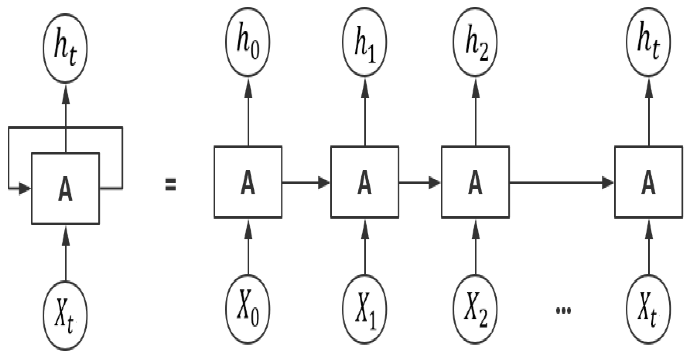
Traditional neural networks have no memory function. Therefore, they fail to use the information that has already appeared at the previous moment. Other than conventional neural networks, RNN is able to store memory since the current output is dependent on the previous computations. The structure of RNN is described in Figure 1.
In Figure 1, a chained neural network represents a recurrent neural network that can be considered as multiple copies of the same neural network, and the neural network at each moment transmits information to the next moment. However, RNN is confronted with the vanishing gradient problem when it stores much memory. To deal with this problem, LSTM is designed.
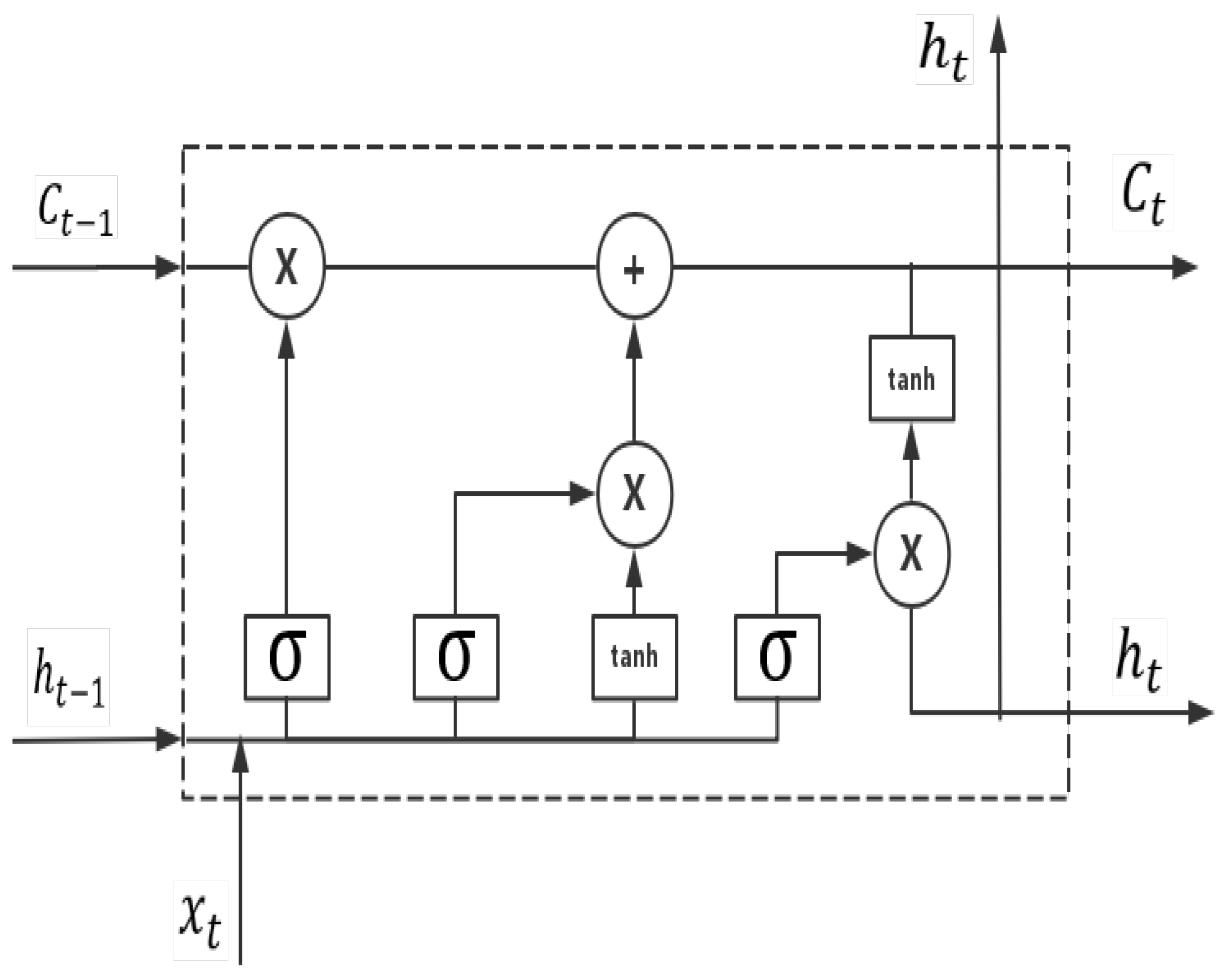
The core of LSTM is the memory block shown in Figure 2. Specifically, the critical components of LSTM are the memory cell and three gates, including the forget gate, input gate and output gate. The LSTM employs the recurrence to represent the input data :
where is the input at time t, is the hidden state at time t and is the hidden state at time .
The calculation of the LSTM network [15] is described as follows:
- (1)
- In line with the previous output and the current input , the forget gate can decide whether to forget the information learned at the last moment in light of Equation (13).
- (2)
- (3)
- The combination of Step (1) and Step (2) is to filter the undesired information and add new information according to Equation (17).
- (4)
- (5)
- The above steps then continue to repeat. The parameter in LSTM can be obtained by maximizing the similarity between the target data and the output of LSTM.
2.4. Variance-Covariance Method
The combination prediction model can utilize the merits of every independent model and promote the prediction accuracy. The key problem of the combination forecasting model is to calculate the weight of each forecasting model. The variance-covariance combined method can find the optimum combination weight coefficient. Therefore, using the variance-covariance combined method can promote the robustness and accuracy for the wind speed forecasting problem.
The variance of every prediction model is calculated as follows:
where n denotes the number of the training set; denote the absolute percentage error for the training data; denotes the average value for . The weights for each forecasting method can be obtained based on the following formula:
In line with the weights for each forecasting method, we can obtain the combined prediction result, which is shown as follows:
where s is the combination prediction result; and are the forecasting results from different methods. Therefore, the variance-covariance method can adjust the corresponding weights dynamically according to the training and test results to obtain a better adaptability.
2.5. The Proposed Forecasting Model
The EEMD method, the LSTM neural network, the GPR method and the variance-covariance method constitute a combination forecasting model. The flowchart of the proposed forecasting model is shown in Figure 3, and the methodology in this study involves the following main steps:
- Step 1:
- The data preprocessing This step includes the data decomposition and the selection for the input of the forecasting method. Original wind speed data are decomposed into various IMFs using the EEMD algorithm. In addition, the PACF method is employed to select the input data of the forecasting method.
- Step 2:
- The prediction for the IMFs LSTM neural network and GPR method with the Bayesian frame of maximum likelihood for parameter optimization are employed to predict the IMFs decomposed by EEMD, respectively.
- Step 3:
- The combination of the two forecasting methods The variance-covariance method is employed to combine the forecasting results from the LSTM neural network and the GPR method.
- Step 4:
- The reconstruction for wind speed information By Equation (5), the prediction result for wind speed is the sum of the predicted IMFs.
3. Case Study
3.1. Collection of Data
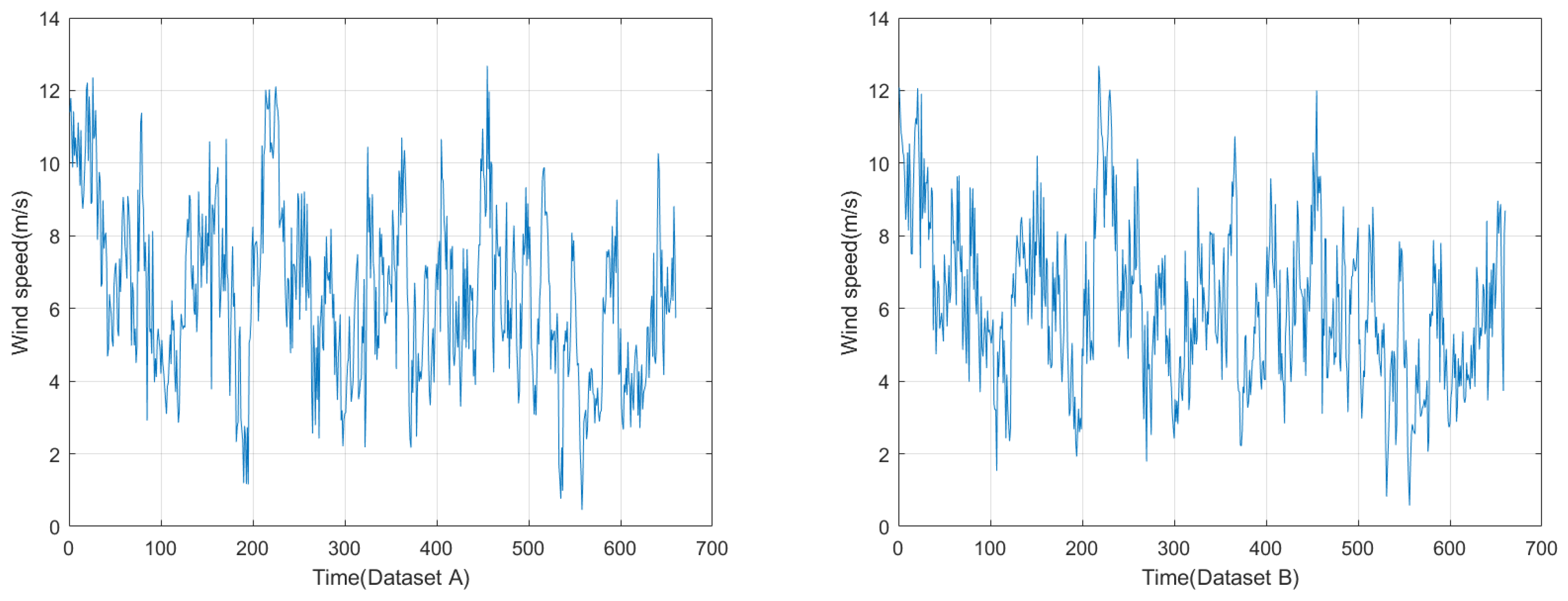
In recent years, Zhangjiakou, North China, has vigorously promoted the development of new energy industry focusing on wind power generation and has become an important new energy industry base in North China. At present, the wind power installed capacity of Zhangjiakou, North China, has reached 8.71 million kilowatts. Therefore, to investigate the wind speed forecasting problem, this paper collects the wind speed data from a wind farm of Zhangjiakou, North China. To consider the effect of different time resolutions, two forecasting cases are represented in this case study. One forecasting case is based on Dataset A, and another forecasting case is based on Dataset B. The data in the Dataset A are recorded every 5 min and from 1 January 2014 to 4 January 2014. Additionally, the data in Dataset B are recorded every 60 min and from 1 July 2014 to 25 July 2014. Therefore, for each forecasting case, the total data groups for each wind turbine reach 660. In these data groups, the former 600 data groups are perceived as a training set, and the rest of data groups are a testing set. The original wind speed series for the two forecasting cases are shown in Figure 4.
3.2. Model Performance Evaluation
In this study, the performance of the proposed model needs to be measured for the comparison with other forecasting models. The mean absolute error (MAE), root mean square error (RMSE) and the mean absolute percentage error (MAPE) are adopted to evaluate the result of the forecasting model.
where denotes the real wind speed data; denotes the wind speed prediction data; .
3.3. Wind Speed Forecasting
Step 1: Wind speed decomposition. The EEMD method is employed to eliminate the non-stationarity of the original wind speed data. The amplitude of the added noise and ensemble number are 0.01 and 100, respectively. The data decomposition results can be seen in Figure 5.
Step 2: Input selection based on PACF. Before the IMFs’ prediction, the input variables of the forecasting method should be determined. The input variables are the time lag of the current wind speed point, since the IMFs are considered as the time series. Hence, the PACF method is employed to determine the number of the time lag. The inputs’ combinations for IMFs identified by the PACF method are illustrated in Table 1.
Step 3: The prediction for IMFs. The LSTM neural network and the GPR method are considered the prediction model for the ten subsequences. The architecture of LSTM and the kernel function in the GPR method have a great influence on the forecasting performance. Specifically, the number of layers and units in LSTM neural network, as well as the form and the parameters of the kernel function in the GPR method need to be determined properly. Therefore, this paper selects a suitable number of layers and units in LSTM for these IMFs and residual series in Table 2. The kernel function of GPR method adopts the squared exponential (SE) function. The values of the parameter in the GPR method optimized by the Bayesian frame of maximum likelihood are shown in Table 3.
Step 4: The combination forecasting method. After obtaining the prediction results for LSTM and the GPR method, this paper uses the variance-covariance method to determine the combination weights of the two forecasting methods. The combination weights for LSTM neural network and the GPR method are 0.66 and 0.34.
3.4. The Comparisons and Analysis
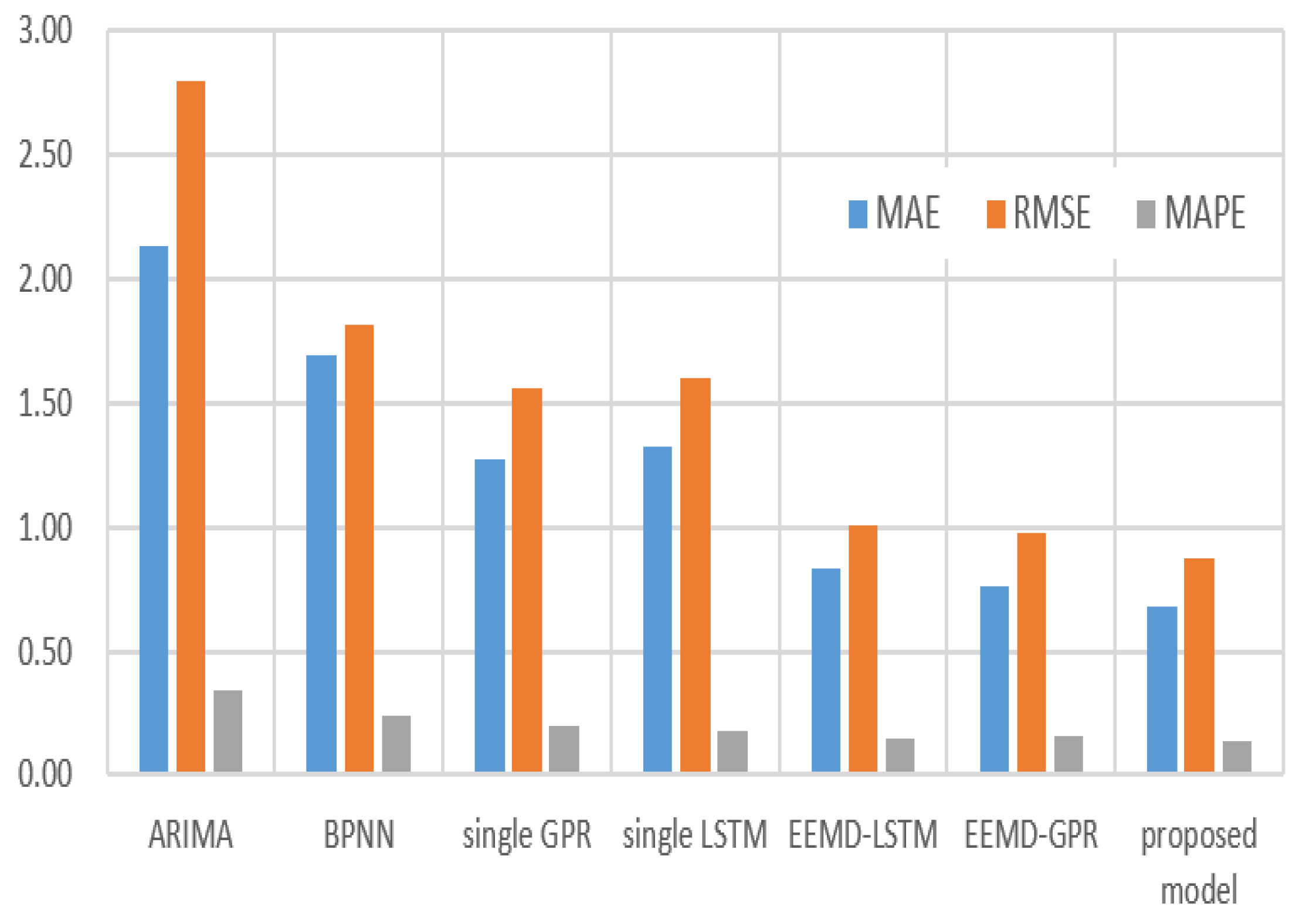
To investigate the performance of the proposed method, the forecasting case in Dataset A has been provided in this paper. Furthermore, six other wind speed prediction methods are also carried out for the comparison with the proposed method. The compared models are ARIMA, BPNN, the single LSTM, the single GPR, EEMD-LSTM and EEMD-GPR. Specifically, ARIMA, BPNN, the single LSTM and the single GPR are utilized for the prediction of the original wind speed data. EEMD-LSTM is the model that employs LSTM to forecast the subsequences decomposed by the EEMD method and reconstructs the IMFs to obtain the wind speed prediction results. In addition, EEMD-GPR is similar to EEMD-LSTM. Based on the IMFs’ prediction results with LSTM and GPR, the proposed model offers a combination forecasting result using the variance-covariance method. Figure 6 displays the real wind speed data and prediction data from different methods in Dataset A. The MAE, RMSE and MAPE values of the above prediction models are given in Figure 7.
As we can see in Figure 7, the MAPE value of the proposed method is 12.10%, while the MAPE values for ARIMA, BPNN, the single LSTM, the single GPR, EEMD-LSTM and EEMD-GPR are 27.65%, 25.05%, 19.18%, 18.33%, 12.29% and 13.17%, respectively. In addition, the RMSE values of ARIMA, BPNN, the single LSTM, the single GPR, EEMD-LSTM, EEMD-GPR and the proposed method are 1.39 m/s, 1.05 m/s, 0.85 m/s, 0.81 m/s, 0.55 m/s, 0.57 m/s and 0.51 m/s, respectively. The MAE value for the proposed method is 0.45 m/s, which is also smaller than that obtained by ARIMA, BPNN, the single LSTM, the single GPR, EEMD-LSTM and EEMD-GPR, which are 1.09 m/s, 0.92 m/s, 0.77 m/s, 0.64 m/s, 0.49 m/s and 0.51 m/s, respectively.
- (a)
- The single LSTM and the single GPR can obtain better results than ARIMA and BPNN. Therefore, it can be concluded that the adopted forecasting methods can obtain higher forecasting accuracy than the conventional forecasting methods, such as ARIMA and BPNN. Additionally, the prediction accuracy of the single LSTM is close to the single GPR.
- (b)
- In comparison with the single LSTM and the single GPR, the EEMD-LSTM and the EEMD-GPR model have better forecasting accuracy obviously. The reason for the forecasting accuracy difference is the EEMD method. It can facilitate the determination of the characteristics of the complex non-linear time series, thereby effectively improving the performance and robustness for wind speed prediction.
- (c)
- By the variance-covariance method, the proposed model combines LSTM and the GPR method to obtain the combination forecasting result. According to the evaluation criteria MAE, RMSE and MAPE, the proposed model outperforms the EEMD-LSTM and the EEMD-GPR model. The combination method can take full advantage of various forecasting models, so the the proposed model can improve the adaptability and accuracy.
- (d)
- The forecasting objective for the proposed method is the wind speed information. As described in Figure 4, the wind speed varies as time changes, and it has strong randomness and instability. In addition, time resolution for wind speed is 5 min or 60 min. Hence, the proposed model can be also applied to forecast short-term time series data, such as short-term wind power and short-term electrical load.
In general, the pro of our suggested method is the improvement in the forecasting performance. Specifically, the EEMD method can facilitate the determination of the characteristics of the complex non-linear time series. Furthermore, the LSTM neural network is suitable for dealing with important events with longer intervals and delays in time series, and the GPR method has a good adaptability and strong generality to process the complex nonlinear problems. To combine the advantages of the two forecasting methods, the variance-covariance method is applied to the proposed method and offers an accurate and stable forecasting result. However, the con of our suggested method is the single form of the kernel function in the GPR method. In the proposed method, we adopt the squared exponential (SE) function. For future work, different kernel functions can be adopted.
3.5. Additional Forecasting Case
To further investigate the performance of the proposed method, another forecasting case in Dataset B has been provided in this paper. The difference between Dataset A and Dataset B is the time resolution. The wind speed data in Dataset A are recorded every 5 min, while the wind speed data in Dataset B are recorded every 60 min. The forecasting results in Dataset B are presented in Figure 8 and Figure 9.
As we can see in Figure 9, the MAPE value of the proposed method is 14.28%, while the MAPE values for ARIMA, BPNN, the single LSTM, the single GPR, EEMD-LSTM and EEMD-GPR are 35.42%, 25.16%, 18.74%, 20.04%, 17.67% and 16.78%, respectively. In addition, the RMSE values of ARIMA, BPNN, the single LSTM, the single GPR, EEMD-LSTM, EEMD-GPR and the proposed method are 1.89 m/s, 1.57 m/s, 1.07 m/s, 1.27 m/s, 1.02 m/s, 0.94 m/s and 0.83 m/s, respectively. The MAE value for the proposed method is 0.67 m/s, which is also smaller than that obtained by ARIMA, BPNN, the single LSTM, the single GPR, EEMD-LSTM and EEMD-GPR, which are 1.57 m/s, 1.19 m/s, 0.84 m/s, 1.02 m/s, 0.79 m/s and 0.71 m/s, respectively.
The prediction results in this forecasting case from Dataset B are consistent with the prediction results in dataset A. Therefore, it can be recommended that the proposed method can adapt to different time resolutions and provide better forecasting results for the short-term wind speed series.
4. Conclusions
To improve the performance of the wind speed prediction, a new combination forecasting model based on the EEMD method, LSTM, GPR and the variance-covariance method is proposed in this paper. The EEMD method is used to decompose the original wind speed series into numerous intrinsic mode functions (IMFs). Then, the variance-covariance method combines the LSTM neural network and the GPR method and offers a combination forecasting result. The results of the case study in Zhangjiakou, China, show that the proposed model tends to outperform other compared prediction models. It is recommended that: (a) the single LSTM and the single GPR can obtain higher forecasting accuracy than the conventional forecasting methods, such as ARIMA and BPNN; (b) the EEMD method can effectively improve the forecasting accuracy by decomposing the original wind speed; (c) the variance-covariance method can combine the advantages of LSTM and the GPR method, and the combination forecasting results are better than the individual prediction method; (d) the EEMD method, the LSTM neural network, the GPR method and the variance-covariance method are integrated reasonably and provide a new idea for short-term wind speed forecasting; (e) the forecasting results in Dataset A and Dataset B indicate that the suggested method can adapt to different time resolutions. In summary, the suggested method in this paper is expected to provide a useful reference for the power sector to forecast the short-term wind speed.
Author Contributions
S.L. had the original idea and wrote the paper. L.Y. provided writing, review and editing. Y.H. provided professional guidance.
Funding
This research was funded by the Fundamental Research Funds for the Central Universities Grant Number 2018QN095.
Acknowledgments
The authors would like to thank the support of the Fundamental Research Funds for the Central Universities Grant Number 2018QN095.
Conflicts of Interest
The authors declare no conflict of interest.
Abbreviations
The following abbreviations are used in this manuscript:
| EEMD | ensemble empirical mode decomposition |
| LSTM | long short-term memory |
| SVM | support vector machine |
| EMD | empirical mode decomposition |
| RNN | recurrent neural network |
| MAE | mean absolute error |
| MAPE | mean absolute percentage error |
| GPR | Gaussian process regression |
| WT | wavelet transform |
| PACF | partial autocorrelation function |
| PACF | partial autocorrelation function |
| CNN | convolutional neural network |
| IMFs | intrinsic mode functions |
| RMSE | root mean square error |
References
- Kumr, Y.; Ringenberg, J.; Depuru, S.S.; Devabhaktuni, V.K.; Lee, J.W.; Nikolaidis, E.; Andersen, B.; Afjeh, A. Wind energy: Trends and enabling technologies. Renew. Sustain. Energy Rev. 2016, 53, 209–224. [Google Scholar] [CrossRef]
- Lu, P.; Ye, L.; Sun, B.; Zhang, C.; Zhao, Y.; Zhu, T. A new hybrid prediction method of ultra-short-term wind power forecasting based on EEMD-PE and LSSVM optimized by the GSA. Energies 2018, 11, 697. [Google Scholar] [CrossRef]
- Muselli, M.; Notton, G.; Cristofari, C.; Louche, A. Forecasting and simulating wind speed in Corsica by using an autoregressive model. Energy Conv. Manag. 2003, 44, 3177–3196. [Google Scholar]
- Shukur, O.B.; Lee, M.H. Daily wind speed forecasting through hybrid KF-ANN model based on ARIMA. Renew. Energy 2015, 76, 637–647. [Google Scholar] [CrossRef]
- Li, G.; Shi, J. On comparing three artificial neural networks for wind speed forecasting. Appl. Energy 2010, 87, 2313–2320. [Google Scholar] [CrossRef]
- Liu, H.; Tian, H.Q.; Li, Y.F.; Zhang, L. Comparison of four Adaboost algorithm based artificial neural networks in wind speed predictions. Energy Conv. Manag. 2015, 92, 67–81. [Google Scholar] [CrossRef]
- Noorollahi, Y.; Jokar, M.A.; Kalhor, A. Using artificial neural networks for temporal and spatial wind speed forecasting in Iran. Energy Conv. Manag. 2016, 115, 17–25. [Google Scholar] [CrossRef]
- Lawan, S.M.; Abidin, W.A.W.Z.; Lawan, S.; Lawan, A.M. An Artificial Intelligence Strategy for the Prediction of Wind Speed and Direction in Sarawak for Wind Energy Mapping; Springer: Singapore, 2016. [Google Scholar]
- Wang, Y.; Wang, J.; Wei, X. A hybrid wind speed forecasting model based on phase space reconstruction theory and Markov model: A case study of wind farms in northwest China. Energy 2015, 91, 556–572. [Google Scholar] [CrossRef]
- Sun, W.; Liu, M.; Liang, Y. Wind speed forecasting based on FEEMD and LSSVM optimized by the bat algorithm. Energies 2015, 8, 6585–6607. [Google Scholar] [CrossRef]
- Hu, J.; Wang, J.; Ma, K. A hybrid technique for short-term wind speed prediction. Energy 2015, 81, 563–574. [Google Scholar] [CrossRef]
- Wang, H.Z.; Wang, G.B.; Li, G.Q.; Peng, J.C.; Liu, Y.T.; Yan, J. Deep belief network based deterministic and probabilistic wind speed forecasting approach. Appl. Energy 2016, 182, 80–93. [Google Scholar] [CrossRef]
- Wang, H.Z.; Li, G.Q.; Wang, G.B.; Peng, J.C.; Jiang, H.; Liu, Y.T. Deep learning based ensemble approach for probabilistic wind power forecasting. Appl. Energy 2017, 188, 56–70. [Google Scholar] [CrossRef]
- Cao, Q.; Ewing, B.T.; Thompson, M.A. Forecasting wind speed with recurrent neural networks. Eur. J. Oper. Res. 2012, 221, 148–154. [Google Scholar] [CrossRef]
- Liu, H.; Mi, X.W.; Li, Y.F. Wind speed forecasting method based on deep learning strategy using empirical wavelet transform, long short term memory neural network and Elman neural network. Energy Conv. Manag. 2018, 156, 498–514. [Google Scholar] [CrossRef]
- Sun, S.; Qiao, H.; Wang, S.; Wei, Y. New dynamic integrated approach for wind speed forecasting. Appl. Energy 2017, 197, 151–162. [Google Scholar] [CrossRef]
- Liu, D.; Niu, D.; Wang, H.; Fan, L. Short-term wind speed forecasting using wavelet transform and support vector machines optimized by genetic algorithm. Renew. Energy 2014, 62, 592–597. [Google Scholar] [CrossRef]
- Fan, G.F.; Peng, L.L.; Zhao, X.; Hong, W.C. Applications of Hybrid EMD with PSO and GA for an SVR-Based Load Forecasting Model. Energies 2017, 10, 1713. [Google Scholar] [CrossRef]
- Wu, Z.; Huang, N.E. Ensemmble empirical mode decomposition: a noise-assisted data analysis method. Adv. Adapt. Data Anal. 2005, 1, 1–41. [Google Scholar] [CrossRef]
- Liu, H.; Mi, X.; Li, Y. Smart deep learning based wind speed prediction model using wavelet packet decomposition, convolutional neural network and convolutional long short term memory network. Energy Conv. Manag. 2018, 166, 120–131. [Google Scholar] [CrossRef]
- Bates, J.M.; Granger, C.W.J. The Combination of Forecasts; Cambridge University Press: Cambridge, UK, 2001; pp. 451–468. [Google Scholar]
- Xiao, L.; Wang, J.; Dong, Y.; Wu, J. Combined forecasting models for wind energy forecasting: A case study in China. Renew. Sustain. Energy Rev. 2015, 44, 271–288. [Google Scholar] [CrossRef]
- Niu, D.; Liang, Y.; Wang, H.; Wang, M.; Hong, W.C. Icing Forecasting of Transmission Lines with a Modified Back Propagation Neural Network-Support Vector Machine-Extreme Learning Machine with Kernel (BPNN-SVM-KELM) Based on the Variance-Covariance Weight Determination Method. Energies 2017, 10, 1196. [Google Scholar] [CrossRef]
- Zhang, H.; Zhu, Y.J.; Fan, L.L.; Qiao-Ling, W.U. Mid-long Term Load Interval Forecasting Based on Markov Modification. East China Electr. Power 2013, 41, 33–36. [Google Scholar]
- Lei, Y.; He, Z.; Zi, Y. Application of the EEMD method to rotor fault diagnosis of rotating machinery. Mech. Syst. Signal Process. 2009, 23, 1327–1338. [Google Scholar] [CrossRef]
- Chalupka, K.; Williams, C.K.I.; Murray, I. A framework for evaluating approximation methods for Gaussian process regression. J. Mach. Learn. Res. 2013, 14, 333–350. [Google Scholar]
- Hu, J.; Wang, J. Short-term wind speed prediction using empirical wavelet transform and Gaussian process regression. Energy 2015, 93, 1456–1466. [Google Scholar] [CrossRef]
- Ying, Z. Asymptotic Properties of a Maximum Likelihood Estimator with Data from a Gaussian Process; Academic Press, Inc.: Cambridge, MA, USA, 1991; pp. 280–296. [Google Scholar]
Figure 1.
The structure of RNN.

Figure 2.
The structure of LSTM.

Figure 3.
The flowchart of the proposed forecasting model.

Figure 4.
Original wind speed series.

Figure 5.
Wind speed series decomposition using EEMD.

Figure 6.
The real wind speed data and prediction data from different methods in Dataset A.

Figure 7.
Wind speed forecasting results in Dataset A.

Figure 8.
The real wind speed data and prediction data from different methods in Dataset B.

Figure 9.
Wind speed forecasting results in Dataset B.


Table 1.
The inputs’ combinations for IMFs.
| IMF | IMF1 | IMF2 | IMF3 | IMF4 | IMF5 | IMF6 | IMF7 | IMF8 | IMF9 | R0 |
|---|---|---|---|---|---|---|---|---|---|---|
| time lag number | 3 | 6 | 7 | 9 | 6 | 8 | 8 | 6 | 3 | 10 |
Table 2.
The number of layers and units in LSTM for each IMF.
| IMF | IMF1 | IMF2 | IMF3 | IMF4 | IMF5 | IMF6 | IMF7 | IMF8 | IMF9 | R0 |
|---|---|---|---|---|---|---|---|---|---|---|
| Layers | 2 | 3 | 1 | 2 | 1 | 3 | 3 | 2 | 1 | 2 |
| Units | 100 | 200 | 50 | 50 | 100 | 200 | 100 | 50 | 200 | 50 |
Table 3.
The parameter in GPR method for each IMF.
| IMF | IMF1 | IMF2 | IMF3 | IMF4 | IMF5 | IMF6 | IMF7 | IMF8 | IMF9 | R0 |
|---|---|---|---|---|---|---|---|---|---|---|
| length scale | 11.9 | 3.1 | 108.4 | 0.01 | 100.9 | 146.4 | 223.3 | 529.7 | 205.6 | 107.7 |
| sigma | 2.2 | 0.5 | 142.2 | 0.02 | 62.5 | 73.6 | 111.2 | 239.0 | 69.6 | 34.2 |
© 2018 by the authors. Licensee MDPI, Basel, Switzerland. This article is an open access article distributed under the terms and conditions of the Creative Commons Attribution (CC BY) license (http://creativecommons.org/licenses/by/4.0/).
Share and Cite
MDPI and ACS Style
Huang, Y.; Liu, S.; Yang, L. Wind Speed Forecasting Method Using EEMD and the Combination Forecasting Method Based on GPR and LSTM. Sustainability 2018, 10, 3693. https://doi.org/10.3390/su10103693
AMA Style
Huang Y, Liu S, Yang L. Wind Speed Forecasting Method Using EEMD and the Combination Forecasting Method Based on GPR and LSTM. Sustainability. 2018; 10(10):3693. https://doi.org/10.3390/su10103693
Chicago/Turabian StyleHuang, Yuansheng, Shijian Liu, and Lei Yang. 2018. "Wind Speed Forecasting Method Using EEMD and the Combination Forecasting Method Based on GPR and LSTM" Sustainability 10, no. 10: 3693. https://doi.org/10.3390/su10103693
Note that from the first issue of 2016, this journal uses article numbers instead of page numbers. See further details here.