Deep Decarbonisation from a Biophysical Perspective: GHG Emissions of a Renewable Electricity Transformation in the EU


1
Institute of Environmental Science and Technology, Universitat Autònoma de Barcelona, 08193 Bellaterra, Spain
2
Catalan Institution for Research and Advanced Studies (ICREA), Passeig Lluís Companys 23, 08010 Barcelona, Spain
*
Author to whom correspondence should be addressed.
Sustainability 2018, 10(10), 3685; https://doi.org/10.3390/su10103685
Submission received: 21 June 2018
/
Revised: 24 September 2018
/
Accepted: 26 September 2018
/
Published: 15 October 2018
(This article belongs to the Special Issue Scenarios and Indicators for Sustainable Development–Towards A Critical Assessment of Achievements and Challenges)
Abstract
:In light of climate change and security concerns, decarbonisation has become a priority for industrialised countries. In the European Union (EU), decarbonisation scenarios used to support decision-making predict a steady decrease in greenhouse gas (GHG) emissions, mostly driven by changes in production mixes and improvements in efficiency. In the EU’s decarbonisation pathways, the power sector plays a large role, reaching zero emissions by 2050. From a biophysical perspective, decarbonisation becomes not just a matter of replacing carbon-intensive with carbon-neutral electricity flows, but also a matter of building and maintaining new infrastructure (funds) which, in turn, is associated with GHG emissions. By not accounting for the emissions associated with funds, particularly those required to increase grid flexibility, scenarios used to inform decarbonisation narratives in the EU are missing a key part of the picture. We show that a rapid and deep decarbonisation of the EU’s power sector through a production-side transition between the years 2020 and 2050 leads to cumulative emissions of the order of 21–25 Gt of CO2 equivalent, within a range of approximately 35–45%. The results are obtained by modelling two decarbonisation pathways where grid flexibility increases either through storage or through curtailment. The analysis suggests that scenarios informing decarbonisation policies in the EU are optimistic and may lead to a narrow focus on sustainable production transformations. This minimises the perceived urgency of reducing overall energy consumption to stay within safe carbon budgets.
1. Introduction
The type of primary energy sources (PES) used by societies to generate a given mix of energy carriers (ECs) is central in shaping their organisation, pace and activities [1,2]. Industrial societies have developed through a heavy reliance on fossil fuels, characterised by their high density. In addition, fossil fuels can be stored and transported across borders, bypassing local natural resource limitations. The exploitation of fossil fuels, while shaping industrial societies’ activities and allowing for a high living standard and rapid rates of urbanisation [3], has also led to unbearable environmental effects, locally and globally. As a consequence, moving away from fossil-based energy systems has become a priority for industrialised economies. In addition to environmental concerns, in the EU, a renewable transformation of the energy system is also desirable from a security of supply perspective, given the lack of indigenous fossil fuels on local territory [4,5,6].
Thus, it has become progressively pressing in the EU to shift to alternative (local) energy sources resulting in lower greenhouse gas (GHG) emissions throughout their lifetime [6]. However, the shift itself has not been easy to initiate, model or govern. The Energiewende is an example of this, having led overall to higher electricity prices and higher emissions, despite strong efforts to shift production patterns of energy carriers [7].
Depending on the chosen problem framing, barriers to a renewable energy transition may be conceived as being of a political, economic, social, institutional or biophysical nature. We borrow the term biophysical from the field of bio-economics, where the economic process is viewed not only through the lens of monetary flows, but most importantly through the lens of flows of biological and physical resources that are produced, distributed, consumed and exchanged [8]. In this sense, the amount of water, emissions and labour associated with a certain energy system, for example, may be categorised as biophysical variables, in opposition to economic ones such as energy prices. Within the field of bio-economics, the term energy metabolism is used to describe the way in which societies extract, process and distribute flows of energy in order to carry out tasks that are crucial to the survival of their identity [9].
Taking a biophysical perspective of the energy system, in this paper we focus on the decarbonisation of the EU’s power sector. Our aim is to provide an alternative narrative to those underpinning EU decarbonisation pathways, where barriers to energy transformations are mostly relegated to the domain of finance and investments [6]. To do this, we model alternative decarbonisation pathways that include the GHG emissions associated with the lifetime of funds. We borrow the distinction between funds and flows from Georgescu-Roegen [8]. Within Georgescu-Roegen’s flow-fund model, given a chosen spatial and temporal scale of analysis, funds are those elements whose identity remains intact, while flows are elements either entering the system without exiting it or exiting it without entering it. From a metabolic perspective, funds are the elements metabolising flows—land, for example, is a fund to be maintained, while the food it grows is a flow. Considering an energy system over a yearly timescale, the electricity and fuels produced and consumed are flows. The infrastructure and human time invested in the production and consumption of flows are the funds of the system.
This distinction is important to study the implications of infrastructural changes in the energy system. The magnitude of infrastructural changes required on the production and consumption side for a decarbonisation of the energy system are not unknown to policymakers [10]. However, there is a tendency within scenarios at the EU’s science-policy interface to use biophysical variables to describes changes in flows (e.g., the amount of electricity consumed over a year) and to adopt a monetary perspective to account for changes in infrastructure (e.g., the investments required to build new transmission and distribution lines). When considering changes associated with funds, a biophysical perspective (e.g., the amount of labour, emissions, water and waste associated with infrastructural changes) is often neglected. This is the case, for example, in the EU 2016 Reference Scenario, where capital investments linked to infrastructure are estimated [11].
Building on data available through existing studies, we developed a scenario singling out the EU power sector up to 2050 and hypothesized two different pathways for its decarbonisation. Increasing grid flexibility is central to ensuring that high levels of variable renewable energy (VRE) can be managed by the grid [12]. In the first pathway, grid flexibility was increased through high rates of curtailment of renewable generation and low storage; in the second, lower levels of curtailment were paired with storage technologies. In each pathway, the emissions associated with the cultivation, construction and fabrication (CFC) of funds were calculated at yearly intervals up to the year 2050, in addition to the operational emissions associated with electricity generation (flows). The approach is meta-analytical and adjusts data available in literature, rather than modelling the behaviour of the grid.
The rest of the paper is organised as follows: Section 2 provides an overview of the decarbonisation pathways currently modelled to support EU decision-making and places them within the wider academic discourses of energy and GHG payback time; Section 3 introduces alternative pathways, with an overview of the underpinning assumptions (Section 3.1) and modelling equations (Section 3.2). The results and discussion are presented in Section 4, split into yearly and cumulative GHG emissions (Section 4.1), variational ranges in results (Section 4.2) and discussion of results (Section 4.3).
2. Background
2.1. Decarbonisation in EU Policy
In the EU, the energy sector accounted for approximately 30% of total emissions in 2016. It was the sector with the highest share of emissions, followed by transport and by manufacturing (accounting for approximately 20% each) [13]. EU decarbonisation policies fall under the 2050 low-carbon economy package [14], as part of the EU’s wider climate strategy. The low-carbon economy roadmap calls for GHG emissions to be cut by 80% below the 1990 levels by 2050, with two intermediate milestones of 40% by 2030 and 60% by 2040. The strategy is currently being renewed in order to reflect the Paris Agreement and is expected to be updated by early 2019 [15].
The EU Energy Roadmap 2050, published in 2011, highlights four strategic directions for decarbonisation: energy efficiency, renewable energy sources (RES), nuclear and carbon capture and storage (CCS). The four directions are explored through six scenarios: current policies, high efficiency, high RES, delayed CCS, low nuclear and diversified supply technologies. Since the publication of the Energy Roadmap 2050, significant events such as the Paris Agreement and the release of the Clean Energy for all Europeans package have impacted EU energy discourses. In light of this, new scenarios have been developed to inform the EU’s mid-century strategy, to be released by fall this year (2018). The scenarios included in the Clean Energy for all Europeans package model pathways to decarbonisation based on efficiency, integration of renewable energy sources and the functioning of the internal energy market [16]. The main trends, which are an increased share of RES, a linear decrease of GHG and an increased electrification, have persisted across the two generations of scenarios.
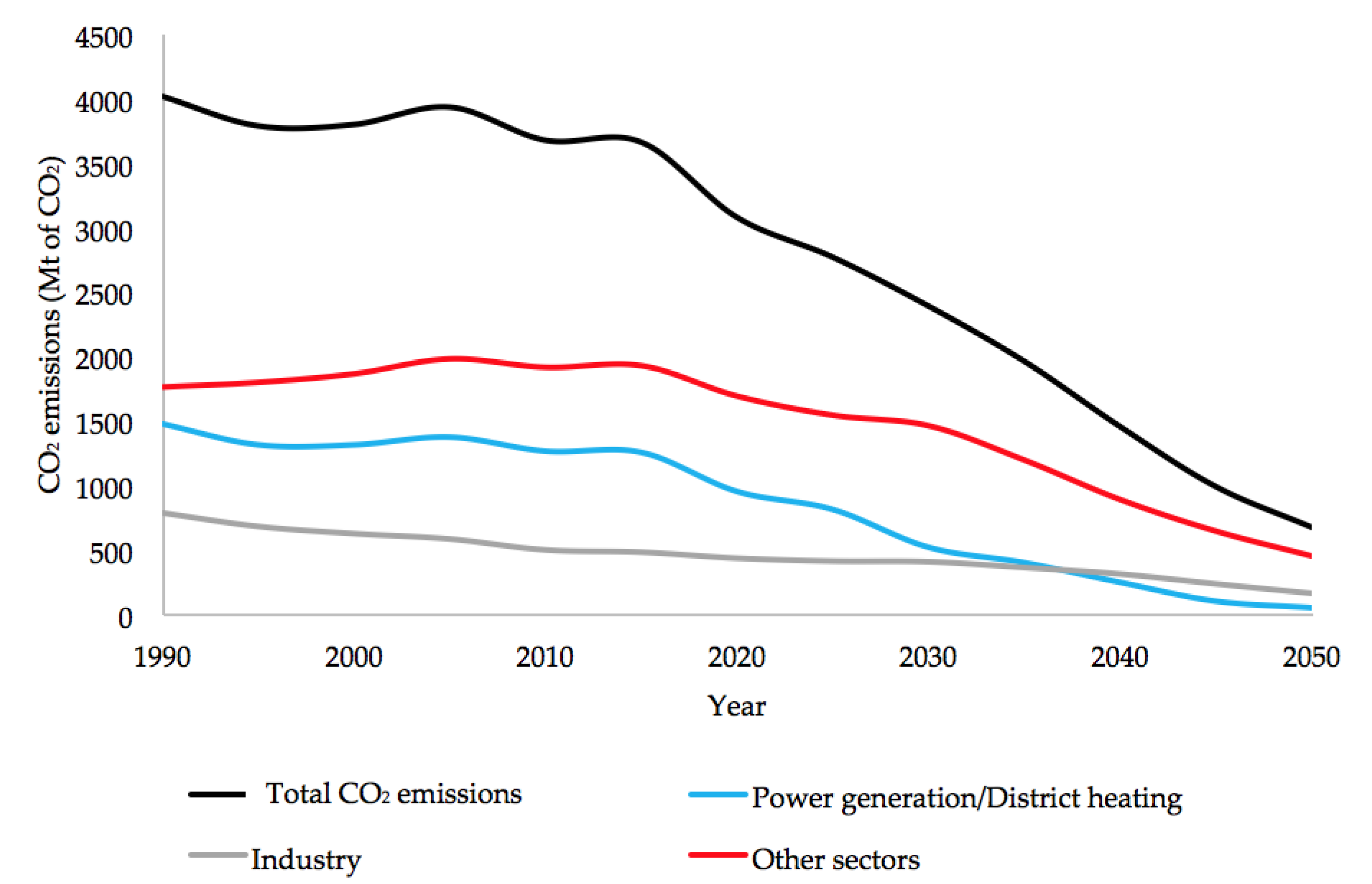
In the six decarbonisation scenarios of the Energy Roadmap 2050, RES rise significantly, to a minimum of 55% of gross consumption of energy carriers in 2050 and 60–80% of gross electricity production by the same year. Absolute electricity production increases steadily between 20 and 40% by 2050 across the six scenarios, despite an overall reduction in total energy consumption. This reflects trends in mitigation scenarios, where a gradual electrification of the energy system is seen as a key element for its decarbonisation [17]. Emissions across all sectors decrease steadily and monotonically—that is, there is no increase in emissions associated with infrastructural change and there are no relative peaks of GHG emissions throughout the years. Figure 1 shows an example of projected sectoral emission reduction in the high RES pathway.
The power sector, in particular, is seen to reach zero or almost zero emissions by 2050 for all pathways, as further indicated by the low-carbon strategy: “The power sector has the biggest potential for cutting emissions. It can almost totally eliminate CO2 emissions by 2050” [14]. Similarly, the Intergovernmental Panel on Climate Change (IPCC) highlights the decarbonisation of the power sector as one of the three main components of mitigation scenario studies, together with a gradual electrification of the energy sector and a reduction in energy demand through technology and other substitutions [17].
The scenarios developed to support the Energy Roadmap 2050 build on the PRIMES (Price-Induced Market Equilibrium System) energy model, “a partial equilibrium modelling system that simulates an energy market equilibrium in the European Union and each of its Member States” [18].
For the accounting of GHG emissions, the model simulates the operational emissions associated with electricity production (a flow) but neglects the emissions associated with the construction of infrastructure (a fund). This omission is linked to the fact that grid flexibility requirements are not modelled. A small but growing body of literature in academia, as highlighted in the next sub-section, points towards the emissions associated with renewable infrastructure and with storage, and to how they may impact future decarbonisation pathways. Additionally, the need to increase grid flexibility at high renewable energy penetrations has been stressed and modelled for specific case studies, including Europe [19], Japan [20], Texas [21] and California [22].
However, EU energy policy discourses uphold the narrative that the main barrier to a high integration of RES into the energy system is financial rather than biophysical. The renewable energy package [6], for example, highlights a number of barriers envisioned on the path to a fully renewable energy system, including administrative hurdles, cost-effectiveness, loss of citizen buy-in and uncertainty for investors. Grid stability is also mentioned as an issue, with the electricity system needing to “adapt to an increasingly decentralized and variable production” [6]. Despite this mention, the issue is not framed as being central and no concrete targets for adaptation have been set, nor have the (biophysical) implications of increasing grid flexibility been included in the EU decarbonisation pathways.
2.2. Energy and GHG Payback Time
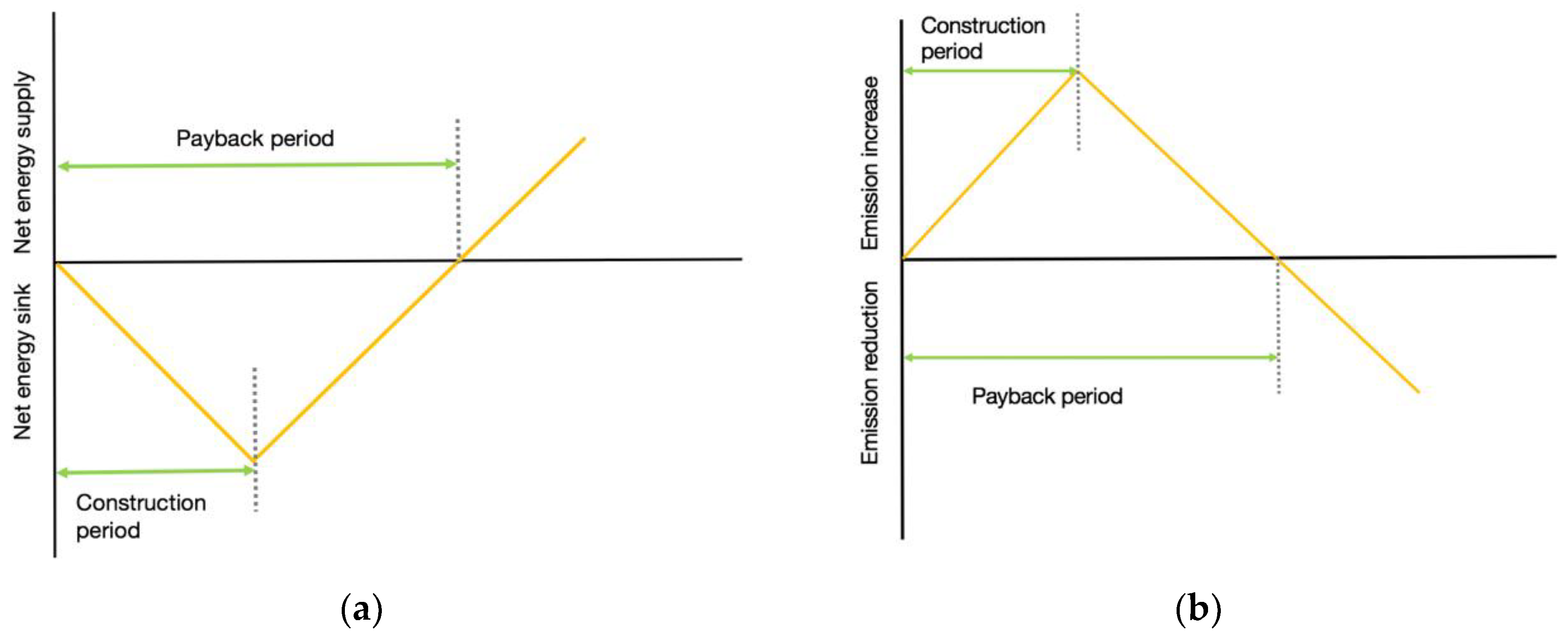
The biophysical investments (such as energy and land) associated with the construction of energy systems have been the subject of a prolific field of energy analysis. The widely used concept of Energy Returned on Energy Invested (EROI) accounts for the amount of net energy generated by an energy system, when the fixed capital and variable operational energy investments required for its construction and maintenance are discounted [23,24]. EROI is particularly relevant for the assessment of alternative energy carriers, such as biofuels, requiring a high energetic investment throughout their production chain [25]. A parallel concept to EROI is the Energy Payback Time (EPBT), accounting for the amount of time it takes for an energy system to break even in terms of the production of energy carriers (in relation to those consumed in its construction). So far, EPBT has been mostly applied to the analysis of solar panels [26,27]. Similar to EPBT, the emissions associated with the construction and operation of energy systems can be accounted for in what is known as the GHG, carbon or environmental payback time (GHGPBT). The GHGPBT indicates the time it takes for a system to become carbon neutral following an initial emission investment due to material extraction, transport and construction [28,29]. Figure 2 shows a schematic view of the concepts of energy and GHG payback time, central to the biophysical accounting of energy systems.
The concepts of energy and GHG payback time can be applied to storage systems. A high penetration of intermittent energy sources into the electricity grid is likely to require a combination of demand-side management, storage infrastructure and improvement of transmission and distribution lines to ensure that intermittent electricity is dispatchable at all times [12]. Studies on storage estimations for a 100% renewable electricity system present high doses of uncertainty, however, the most thorough reviews point towards storage needs greatly beyond what is currently operational at the global scale [20,21,22]. Thus, the importance of being able to assess and compare the performance of storage systems has become evident. Building on the idea of EROI, Barnhart and Benson [30] introduced the concept of Energy Stored on Energy Invested (ESOI), accounting for the amount of net energy output provided by storage technologies compared to the energy invested in their construction and operation. Battery technologies show a performance approximately 20 times lower (in terms of ESOI) than compressed air energy storage (CAES) and pumped hydroelectric storage (PHS). However, due to the invasive nature of CAES and PHS and due to the strong limitations to their expansion brought by geographic configurations, batteries have become a popular option in the discussion of storage futures [31].
In a biophysical framing, the GHG emissions of storage technologies throughout their lifetime are a key element in the assessment of future energy scenarios. A thorough review by Denholm [31] showed how PHS is associated with the lowest amount of emissions over its lifetime, while batteries are associated with non-negligible lifetime emissions. In its present form, CAES relies on the use of natural gas and therefore also presents non-negligible lifetime emissions.
Similar to the emissions of storage infrastructure, the GHG emissions associated with the lifecycle of renewable infrastructure have been studied—see Nugent and Sovacool [32] for a thorough review of the topic. The emissions associated with renewable electricity generation over its lifetime are considerably lower than those associated with fossil electricity. As a consequence, not much attention has been placed in exploring the nuances of different pathways and storage options in terms of their associated emissions. Crucial questions regarding the best pathways to decarbonisation in relation to emission curves, thus, remain underexplored [32].
3. Alternative Decarbonisation Pathways
When dealing with complex systems, such as the social-ecological one, modelling may have two purposes: To predict and control future states of the system or to better understand the current one [33]. As the high doses of uncertainty attached to the prediction of future states of the complex social-ecological system become apparent, scenarios used to support decision-making are framed more and more as tools for deliberation, rather than prediction. The EU webpage on energy modelling, for example, states that the EU Reference Scenario, “one of the European Commission’s key analysis tools in the areas of energy, transport and climate action”, (…), “is not designed as a forecast of what is likely to happen in the future but it provides a benchmark against which new policy proposals can be assessed” [34]. In a similar spirit, the aim of the alternative decarbonisation pathways is not to predict the behaviour of future decarbonisation pathways in the EU. Rather, the aim is to flag the need to include emissions associated with the construction of infrastructure in decarbonisation discourses. This is particularly relevant for intermittent sources of energy and their grid flexibility requirements.
We explored two decarbonisation pathways of the EU’s power sector for the years 2020–2050, each dealing differently with grid flexibility requirements. Focus was given to the integration of renewable energy into the grid as a means to decrease GHG emissions, in line with the high RES scenario of the EU’s Energy Roadmap 2050, on which the two pathways were based. The values of gross electricity consumption up to 2050, in fact, were taken from the high RES scenario, as well as the share of nuclear electricity at each year. Hydropower was assumed to remain unchanged over the years, while solar power and wind power were assumed to increase until producing 90% of electricity, entirely phasing out fossil power plants. Adjusting data from existing studies, we calculated the emissions associated with the construction and operation of funds (renewable and storage infrastructure) with respect to the reduction in emissions due to the substitution of fossil with alternative energy systems (associated with the electricity generated by the systems—flows).
3.1. Modelling Assumptions
Any model informing the future behaviour of energy systems necessarily relies on heavy sets of assumptions regarding technology, consumption and production patterns. Modelling assumptions of the alternative decarbonisation pathways are split into two sections: grid flexibility and GHG emissions.
3.1.1. Grid Flexibility
Integrating high levels of variable renewable energy (VRE), such as the electricity produced by wind turbines or solar photovoltaic (PV) panels, into the grid requires an increase in the flexibility of the grid. Grid flexibility can be achieved in various ways. Kondziella and Bruckner [12] identified seven possible measures on the production and on the consumption side: highly flexible power plants, large-scale energy storage, curtailment of renewable surplus, demand-side management, grid extension, virtual power plants and linkage of energy markets. These measures, either individually or in unison, can ensure that electricity demand is met at all times. Here, focus was given to the production-side measures of large-scale energy storage and of the curtailment of renewable surplus.
Existing studies [12,19,20,21,22,35,36] show that increasing grid flexibility becomes essential when the share of VRE fed into the grid reaches levels of 40 to 50%. Grid flexibility can be increased through large-scale energy storage. In this case, surplus electricity generated by VRE when production is higher than demand can be converted into gravitational, thermal or electrochemical energy and fed back into the system when production is lower than demand. Curtailment of renewable surplus, on the other hand, relies on the installation of more renewable infrastructure than what is needed to cover average yearly demand (also known as backup power plants). When the combined electrical output of the renewable infrastructure is higher than the demand at a given point in time, the output of VRE plants is curtailed. As a result, curtailment of renewable surplus as a means to improve grid flexibility has an impact on the utilisation factor (UF) of renewable plants. The review paper by Kondziella and Bruckner [12] provided a thorough overview of existing studies assessing grid flexibility requirements for high renewable integration.
Steinke [19] examined the interplay between storage, curtailment and grid extensions for a 100% renewable electricity system in Europe. Denholm and Hand [21] and Denholm and Margolis [22] modelled, respectively, the electricity grids of Texas and California to provide an assessment of how grid flexibility can be achieved in low and high storage scenarios. The models of US case studies, produced for the National Renewable Energy Laboratory (NREL), have not been replicated in the EU to this level of detail and are the most comprehensive reference points for assessments of grid flexibility. Building on these studies [21,22], we hypothesised two pathways for decarbonisation: a low storage high curtailment (LSHC) pathway and a high storage low curtailment (HSLC) one. In the former, we assumed that no extra storage technologies were added to the EU’s electricity system, therefore the only storage services available up to 2050 were those produced by current PHS facilities (at a storage capacity of approximately 600 GWh [37]). To ensure grid flexibility, renewable back up power was added and renewable generation was assumed to be curtailed. In the latter, curtailment was greatly decreased by the addition of storage services. Both scenarios adapted the curtailment and flexibility rates from the comprehensive model of the Texas grid [21]. The relations between curtailment and flexibility in the EU depend on specific geographies and grid configurations. However, for the purpose of these pathways—i.e., to point towards a problem in GHG accounting rather than to provide accurate predictions—this approximation was considered satisficing.
The total amount of storage required by 2050 was calculated following Steinke [19] and Renner and Giampietro [35]. Assuming that grid expansions were limited to the national scale and that no backup generation was provided, Steinke estimated that the EU would require between 7 and 30 days of storage to accommodate shares of 90% or more of VRE. Analysing data for Germany and Spain over an 84 months and 132 months, with a resolution of 60 minutes and 10 minutes respectively, Renner and Giampietro estimated that the two countries would require approximately one week of storage capacity in a 100% intermittent penetration scenario. The study used the comprehensive datasets available for the two countries to check “the extent of the predicted worst annual hypothetical ‘failure event’ (where the guaranteed level of intermittently sourced electricity is not met)”. The results by Renner and Giampietro for Germany are in line with the analysis by Kuhn [36], predicting a requirement of installed storage charging power in Germany of the order of 53 GW by 2050. Similar values apply to the case of Japan [20], where, despite a different energy mix and configuration, it was also found that storage requirements are on the order of a week of average electricity supply.
Thus, storage capacity requirements for 2050, where gross electricity production is assumed to grow to approximately 5140 TWh, were assumed to be on the order of a week of average daily demand. It was then assumed that PHS, the most implemented and mature storage technology in the EU and worldwide, increased up to its viable potential in the EU, following the analysis by Gimeno-Gutiérrez and Lacal-Arántegui [38]. Then, battery energy storage (BES) was introduced to cover the gap between the maximum PHS potential and the total storage capacity needed. The relevant assumptions shared across pathways and those differing for each pathway are collected in Table 1 and Table 2 respectively, at ten-year snapshots between 2020 and 2050.
Following the EU high RES pathway, gross electricity consumption increased in both pathways, despite an overall reduction in energy consumption—mirroring the trend of electrification. Hydropower (excluding PHS) was assumed to remain unchanged throughout the years, therefore as electricity generation increased its share in the electricity mix decreased. Nuclear power was assumed to gradually decrease in absolute and relative terms. All other non-renewable power plants were grouped under the umbrella term fossil plants and eliminated by 2050. The share of wind and solar power rose gradually until reaching 90% of the total generation share in 2050. The relative contribution of wind and solar power remained fixed at 70 and 30% respectively, mirroring their 2016 relative contribution in the EU. This was also in line with what was identified by Denholm and Hand [21] as the optimal balance between the two types of generation technologies to ensure minimum curtailment.
Given the higher curtailment rate in the LSHC scenario, although the gross electricity consumption was the same as in the HSLC scenario, a higher amount of wind and solar power were assumed to be generated (see the second and third row of Table 2). The surplus generation was not assumed to enter the grid but was curtailed. The curtailment rates, also included in Table 2, were taken from Denholm and Hand [21], by assuming that curtailment rates as a function of VRE penetration can be generalised. Contrary to storage requirements, which tend to increase linearly as VRE integration increases, curtailment increases exponentially, meaning that it becomes less and less favourable to rely on curtailment at higher rates. The amount of storage capacity, in GWh of installed capacity, did not increase throughout the years for the LSHC scenario. Eurostat does not provide statistics on storage capacity, and the value of 600 GWh of PHS in the EU was taken from Kougias and Szabó [37]. In the HSLC scenario, the storage capacity increased up to a week of average demand. The curtailment rates in both scenarios led to a gradual decrease in the utilisation factors (UF) of wind and solar power, calculated as the amount of time throughout the year when electricity generated by wind and solar (GWhused) was fed into the grid:
where GWinstalled is the installed power capacity, and 8760 is the number of hours in a year.
3.1.2. GHG Emissions of Renewable Infrastructure, Storage and Fossil Plants
The values of lifetime GHG emissions of renewable infrastructure, and their associated ranges, were adjusted from the comprehensive meta-review by Nugent and Sovacool [32]. For GHG emissions of storage technologies, values were taken from Denholm and Kulcinski [39]. Table 3 summarises the main technological assumptions of both studies. For renewable infrastructure, Nugent and Sovacool provide intensive data derived from a number of studies, each with different technical specifications. Therefore, the values do not refer to specific technological characteristics. This enlarges the range of the estimated values, but also their robustness. Storage infrastructure values, similarly, refer to a review of various existing plants, with the range of technological characteristics included in Table 3. As the GHG emissions associated with battery energy storage (BES) were an important variable for the results, the values of Denholm and Kulcinski, dating to 2004, were cross-checked against a recent study referring specifically to lithium-ion batteries [40]. and were found to be consistent. Since the scenarios were modelled at the EU level, they did not take into account differences across member states. The values taken from literature, associated with a range of technological characteristics, reflect the heterogeneity of infrastructure required across the EU.
The GHG emissions from the review studies were adjusted as the renewable share of the electricity mix in the pathways increased, since the electricity mix strongly affects GHG emissions. As we were singling out the power sector, emissions associated with the use of fuels and other forms of thermal energy remained invariant. To adjust the values throughout the years, the carbon intensity of the EU’s electricity mix was estimated each year, starting from 320 g/kWh in 2016 [41] and reaching almost zero in 2050. The contribution of the electricity mix to the overall GHG emissions of wind power infrastructure was estimated by comparing existing studies which made a direct link between the carbon intensity of the electricity production system and the GHG emissions associated with infrastructure (see Reference [42] for a comparison of Germany and China, Reference [43] for Brazil and Reference [44] for different values of carbon intensities). The effect of different electricity mixes on the construction on the lifetime of solar panels was assessed directly by Reich [45] in relation to the CO2 emission factor of electricity supply. Varying GHG emissions for CFC and Operation are included in Table 4.
3.2. Modelling Equations
The values of GHG emissions at a given year were calculated from the secondary data, adjusted to the EU’s electricity mix for each year, through the following equations:
where:
GHG_stn = GWPV,n × GHG_stPV,n + GWwind,n × GHG_stwind,n + GWPHS,n × GHG_stPHS,n + GWBES,n × GHG_stBES
GHG_opn = GWhPV,n × GHG_opPV,n + GWhwind,n × GHG_opwind,n + GWhPHS,n × GHG_opPHS,n + GWhBES,n × GHG_opBES + GWhfossil,n × GHG_opfossil,n
- GHG_stn are the GHG emissions, in tons of CO2 equivalent, emitted at year n due to the cultivation, fabrication and construction (CFC) of infrastructure;
- GWPV and GWwind are the amounts of extra solar PV and wind power capacity installed each year;
- GWhPHS and GWhBES are the amounts of extra storage capacity, PHS and BES, added each year;
- GHG_opn are the varying infrastructure emissions at each year n, depending, in turn, on the electricity mix and expressed in tons of CO2 equivalent/GW for renewable infrastructure and tons of CO2 equivalent/GWh for renewable infrastructure;
- GWhn is the electricity generation at year n by each technology.
Similarly, the emissions due to the operation of power plants were calculated at each year as the total amount of electricity generated by each type of power plant (including curtailed electricity) times the associated operational emissions. The total GHG emissions at year n, thus (GHGtotal,n) were a combination of multiple factors varying across the years. What we refer to as cumulative emissions, finally, is the sum of the emissions over the 2020–2050 time period:
4. Results and Discussion
The results and discussion are structured in three sections. Firstly, the yearly and cumulative emissions of the decarbonisation pathways are presented and linked to EU decarbonisation scenarios, and carbon budgets (Section 4.1); then, variational ranges of the results are discussed (Section 4.2). Section 4.3, finally, discusses the role played by biophysical variables at the science-policy interface.
4.1. GHG Emission Curves and Cumulative Emissions
To discuss the results of the two decarbonisation scenarios, emissions can be viewed from three perspectives:
- Emission curves at a yearly resolution, useful to comment on the temporal behaviour of emissions and their possible non-linear evolution;
- Cumulative emissions up to the year 2050, i.e., the sum of the yearly emissions, which can be related to carbon budgets;
- Yearly emissions at the target year 2050, currently the only view used to inform EU decision-making processes (with different targets set for different years).
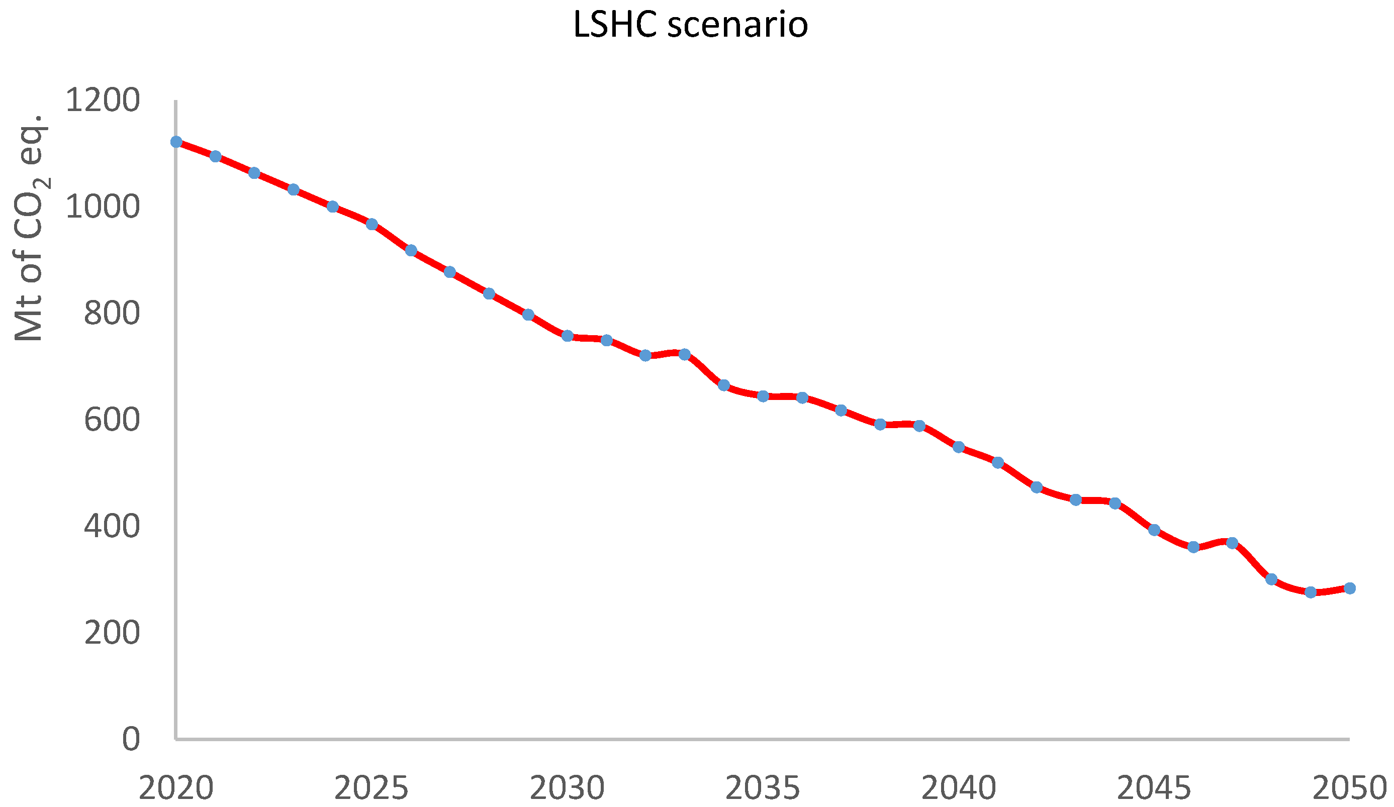
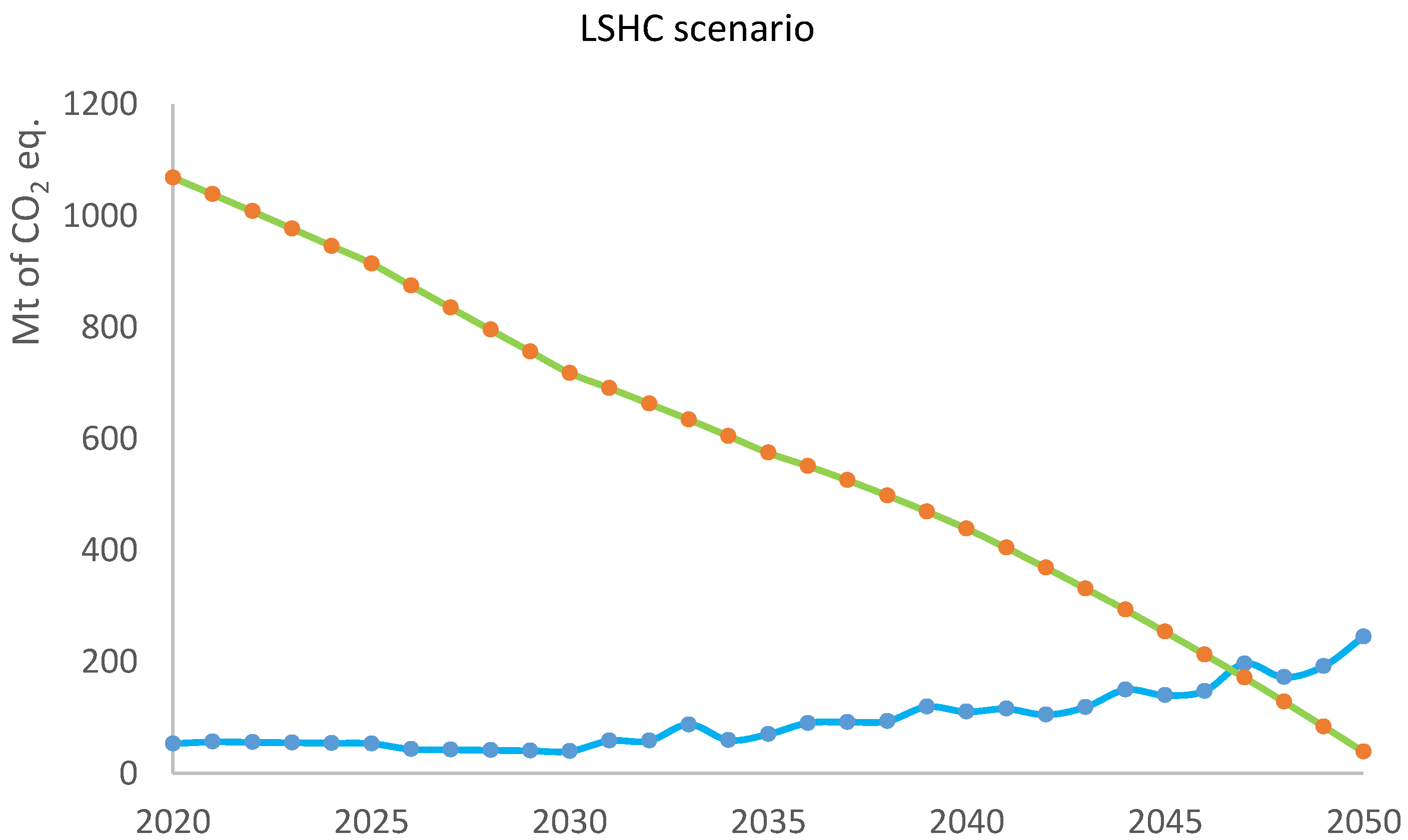
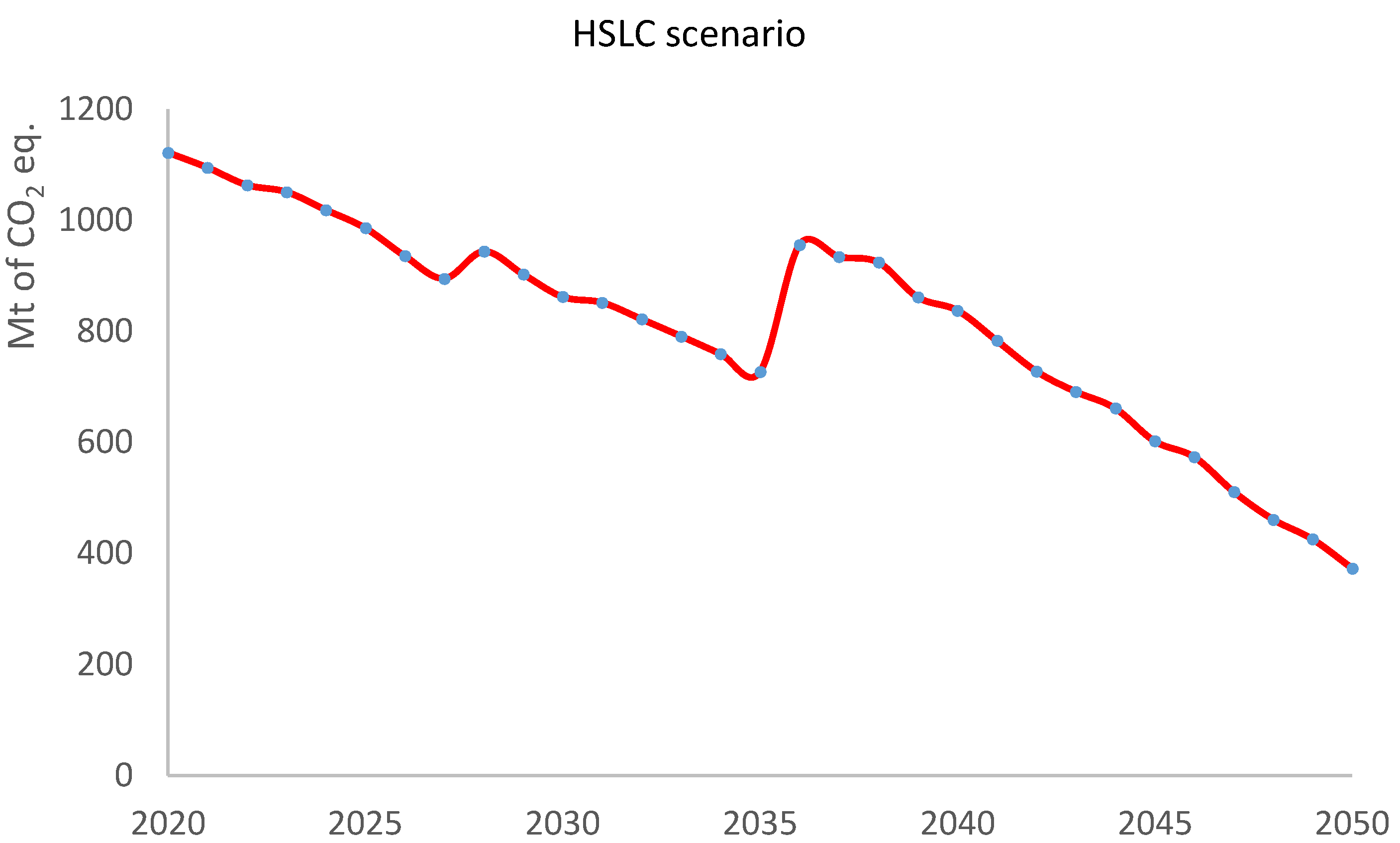
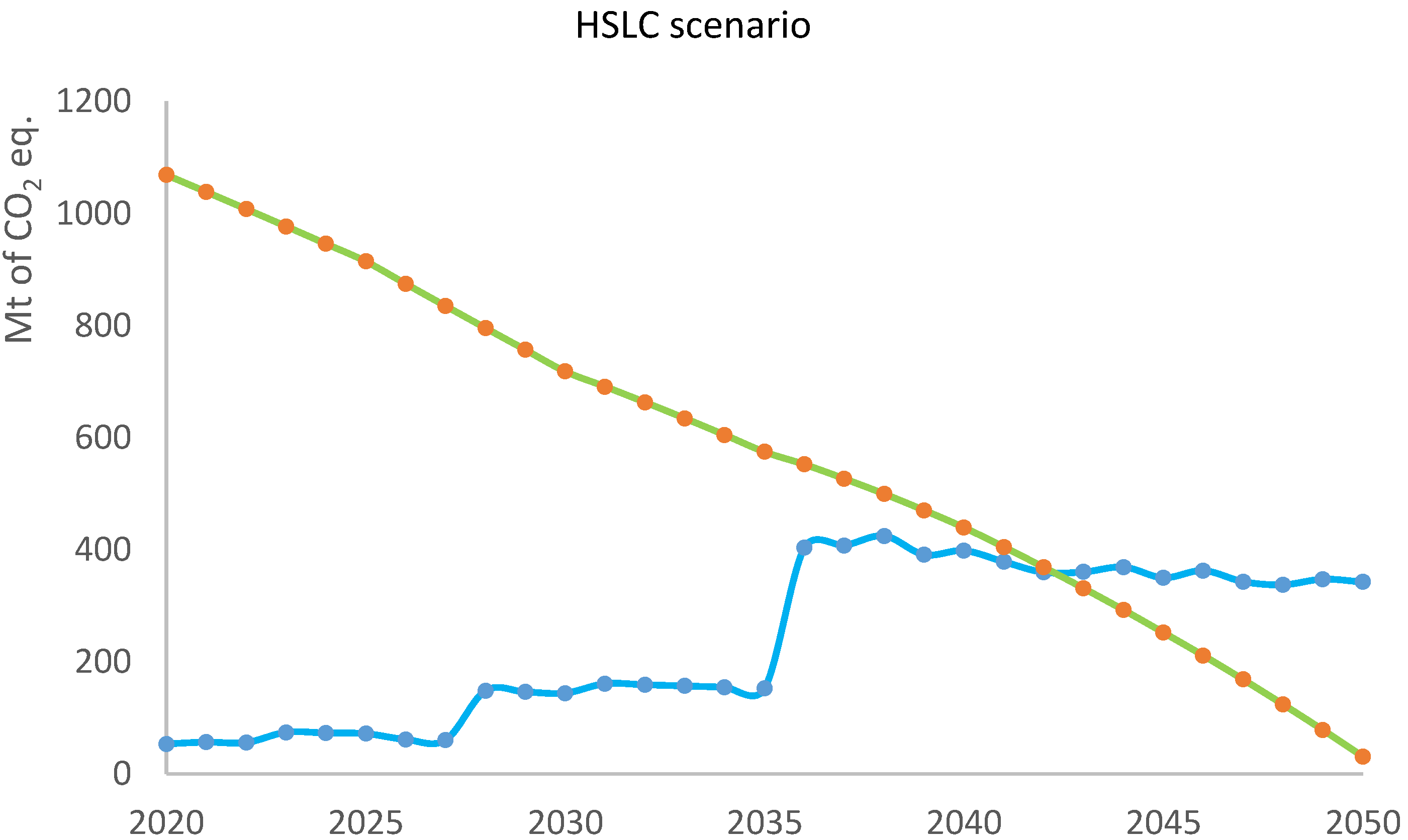
Starting with the emission curves provided throughout the years, Figure 3 and Figure 4 show the behaviour of the GHG emissions of the EU power sector (including cultivation, fabrication and construction of infrastructure) under the low storage high curtailment (LSHC) scenario. The total emissions are shown in Figure 3, while Figure 4 breaks the emissions down into those linked to the operation of power plants (associated with electricity flows) and those linked to the cultivation, fabrication and construction of renewable infrastructure (associated with funds).
In the LSHC scenario, while the amount of wind and solar infrastructure installed each year increased exponentially (see Table 2), the GHG emissions associated with the cultivation, fabrication and construction phases of the infrastructure were mitigated by the steady reduction in operational emissions, which dropped to almost 0 by 2050. The initial steady decrease in emissions became less linear from the year 2030, i.e., when curtailment of renewable electricity started. As curtailment increased, emissions due to an infrastructure rise led to relative peaks in emissions between the years 2030 and 2050, with overall emissions associated with infrastructure increasing despite the increased renewable penetration into the system. The behaviour of the curve depended on the rate that renewable infrastructure was installed.
With high levels of emissions associated with the installation of both PHS and BES storage technologies (see Table 3), the yearly emission curve for the low curtailment high storage (LCHS) scenario displays a behaviour which is less linear, as seen in Figure 5 and Figure 6.
Emissions were strongly dependent on the type of storage infrastructure and on when it was integrated into the system. Emissions gradually decreased up to the year 2027, when the amount of installed PHS started to increase considerably. The biggest peak, however, was visible at the year 2035, when BES technologies were introduced, as PHS reached its maximum capacity. The peak can be softened if BES is gradually installed from the start, however, in this case, cumulative emissions would be higher as the manufacturing process would rely more heavily on fossil fuels. Thus, different timing options should be carefully considered from a biophysical perspective.
The behaviour of the curves of Figure 3 and Figure 5, and the presence or absence of relative GHG emission peaks, can be varied by varying assumptions on timings and introduction of technologies. This would also vary cumulative emissions, as the emissions associated with the construction of infrastructure also depend on the yearly electricity mix. Cumulative emissions are a useful indicator as they can give us an idea of how much is being emitted by the EU’s power sector during its transitional phase towards deep decarbonisation. It is expected that, on average, the EU has a carbon budget on the order of 90 Gt in order to remain within a 2° temperature range for the period between 2020 and 2100 [46]. Cumulative emissions associated with the power sector and to the manufacturing of infrastructure were of the order of 20,830 Mt of CO2 eq. and 25,150 Mt of CO2 eq. respectively, for the HCLS and LCHS scenarios. Thus, under deep decarbonisation pathways, between the years 2020 and 2050 alone the power sector and its associated manufacturing would emit 23–28% of the total budget available to the whole society up to the year 2100. As we discuss in Section 4.3, this suggests that efforts on the production side of the energy system are not enough to stay within safe carbon budgets.
4.2. Analysis of Variational Ranges in the Results
The scenarios presented in this paper build on secondary data collected and adjusted at different levels of the energy system, from individual technologies to systemic production and consumption patterns, expressed in the form of estimate ranges. Table 5 collects the estimate ranges associated with the main variables in the analysis, for the years 2020 and 2050. Table 6 shows how much each variable contributes to the cumulative emissions at the years 2020 and 2050, reflecting the weight that the variable’s estimate range holds in the final interval.
The interval associated with the assessments of yearly operational and infrastructural GHG emissions is determined by a combination of estimate ranges associated with GHG emissions in the base year from which the data is taken and the estimate range associated with the adjustment of emissions as renewable penetration increases, using the squaring method for error propagation. At a higher level, the interval associated with the assessment of consumption patterns can be checked by calculating the lowest and highest values of electricity consumption present in the six EU decarbonisation scenarios. The factors playing the largest impact on the final cumulative GHG emission assessments are the GHG emissions associated with storage infrastructure, curtailment rates and the maximum PHS potential in the EU. Combining the various ranges into the final assessment of cumulative emissions leads to intervals on the order of 35% for the high curtailment scenario and 45% for the high storage scenario. This value is high, especially when it comes to storage GHG emissions and estimations of storage requirements, however, it does not weaken the main message of the analysis.
4.3. Discussion
To inform decision-making, the type of GHG accounting proposed here is incomplete, as it needs to be associated with economic analyses and with the assessment of other biophysical variables such as land and water. While the high curtailment scenario results in overall lower emissions than the high storage one, it would lead to other trade-offs in different domains, including higher electricity prices and large areas of land occupied by renewable infrastructure. On the other hand, the high storage scenario would also be associated with high levels of lithium requirements (to be imported), which may not be desirable from a security perspective. Additionally, increasing PHS to its maximum potential may have important consequences for natural water cycles. Synergies and trade-offs also emerge within and outside EU borders. A part of the emissions derived in the scenarios would necessarily be located outside of EU borders, such as those for the extraction of primary materials. This points towards the need of discussing the impact of EU climate targets at different geographical scales.
When it comes to the integration of renewable energy, differences across countries are also important and should be modelled in relation to grid flexibility and associated GHG emissions. The Netherlands, for example, is mostly flat and does not have any PHS potential, therefore in an increased flexibility scenario, it would either require high rates of curtailment (which may interfere with current land use patterns) or high interconnections to neighbouring countries. Utilisation factors of technologies also vary across countries, depending on weather conditions. In addition to differences across spatial scales, the temporal scale is also important when considering decarbonisation scenarios: different types of storage services, in fact, are useful for fluctuations occurring at different scales [47]. Current statistics do not allow for this type of analysis. Therefore, it would be advisable for supra-national statistical bodies such as Eurostat to include data across shorter timescales.
The results presented are considered to be conservative, as two elements which have not been included in the model may increase GHG emissions substantially: (i) the change in end-use infrastructure required by an increased electrification of the energy sector (such as the manufacturing of electric cars); and (ii) the turnover of funds. There is uncertainty associated with the possible lifetime of grid-scale batteries [47], however, it is likely that within the 30-year timeframe considered in the study some turnover will be necessary, by either producing new batteries or recycling existing ones.
Accounting for the emission flows associated with funds leads to higher emissions than those envisioned by current scenarios. Thus, results suggest that sustainable production narratives cannot alone lead to a decarbonisation of the energy sector. To be effective, sustainable production efforts must be paired with strong efforts for sustainable consumption [48]. These should not only be spurred by mechanisms such as efficiency and technology but also, and crucially, by radical changes in consumption patterns. This is line with the metabolic view of society [49], which draws a clear connection between production and consumption patterns: changes in the way in which energy carriers are produced inevitably require changes in the way in which they are consumed. This may entail a shift not only in how things are done (structural changes, e.g., technology and efficiency) but also in what is done and why (functional changes, e.g., who is consuming what energy, to do what).
5. Conclusions
Fighting climate change, reducing air pollution and increasing security are three entangled priorities of the EU. Decarbonisation has become a central strategy to deal simultaneously with these disparate targets. However, governing a shift to a decarbonised economy has not been simple. We suggest that this difficulty is partly due to the framing of models used to inform deliberative processes. A focus on the monetary aspects of funds, particularly infrastructure, rather than on the biophysical ones, such as GHG emissions, has minimised discourses linked to the magnitude of the material transformations required to restructure the energy system.
Focusing on the EU power sector in the years 2020–2050, we modelled two decarbonisation pathways in relation to GHG emissions. The scenarios consider operational GHG emissions of electricity generation, as well as those associated with the lifetime of renewable and storage infrastructure. Contrary to the decarbonisation pathways used to inform EU decision-making, the alternative decarbonisation pathways take into account grid flexibility requirements from a biophysical perspective. For the chosen pathways, this entails accounting for the GHG emissions associated either with high rates of curtailment or with storage infrastructure. The results show how emission curves behave differently under different flexibility pathways, and relative peaks of GHG emissions across the years, as well as overall higher cumulative emissions, may emerge depending on the set of assumptions.
Many questions arise from a biophysical problem framing of decarbonisation, for example: What is the best timing to implement technologies? What are the trade-offs among different technological pathways and storage solutions? What trade-offs may emerge between local and global environmental effects? By suggesting that a rapid decarbonisation of the EU power sector by 2050 is “feasible and viable” [14], and therefore glossing over biophysical obstacles to renewable transformations, the scientific tools informing EU decision-making do not open up a space to discuss these crucial issues.
Author Contributions
Conceptualization, M.G., L.J.D.F. and M.R..; Methodology, M.R. and L.J.D.F.; Formal Analysis, L.J.D.F.; Data Curation, L.J.D.F..; Writing-Original Draft Preparation, L.J.D.F. and M.G.; Writing-Review and Editing, L.J.D.F., M.G. and M.R.; Supervision, M.G. and M.R.
Funding
The authors acknowledge support by the European Union’s Horizon 2020 research and innovation programme under grant agreement no. 689669 (MAGIC). The Institute of Environmental Science and Technology (ICTA) has received financial support from the Spanish Ministry of Economy and Competitiveness through the “María de Maeztu” program for Units of Excellence (MDM-2015-0552). This work reflects the authors’ view only; the funding agencies are not responsible for any use that may be made of the information it contains.
Acknowledgments
The authors are very grateful to Ansel Renner for providing support in calculating storage requirements, and to three anonymous reviewers for greatly improving the quality of the paper with their thoughtful feedback.
Conflicts of Interest
The authors declare no conflicts of interest.
References
- Smil, V. Energy Transitions: History, Requirements, Prospects; Praeger: Santa Barbara, CA, USA, 2010; ISBN 9780313381775. [Google Scholar]
- Cottrell, F. Energy and Society: The Relation between Energy, Social Changes, and Economic Development; McGraw-Hill: New York, NY, USA, 1955. [Google Scholar]
- Giampietro, M.; Mayumi, K.; Sorman, A. The Metabolic Pattern of Societies: Where Economists Fall Short; Routledge: London, UK, 2011. [Google Scholar]
- European Commission. European Energy Security Strategy; European Commission: Brussels, Belgium, 2014. [Google Scholar]
- Vahtra, P. Energy security in Europe in the aftermath of 2009 Russia-Ukraine gas crisis. In EU-Russia Gas Connection: Pipes, Politics and Problems; Pan European Institute: Turku, Finland, 2009; pp. 159–165. [Google Scholar]
- European Commission. Proposal for a Directive of the European Parliament and of the Council on the Promotion of the Use of Energy from Renewable Sources (Recast); European Commission: Brussels, Belgium, 2017; Volume 0382 (COD), pp. 1–116. [Google Scholar]
- Scholz, R.; Beckmann, M.; Pieper, C.; Muster, M.; Weber, R. Considerations on providing the energy needs using exclusively renewable sources: Energiewende in Germany. Renew. Sustain. Energy Rev. 2014, 35, 109–125. [Google Scholar] [CrossRef]
- Georgescu-Roegen, N. The Entropy Law and the Economic Process; Harvard University Press: Boston, MA, USA, 1971. [Google Scholar]
- Giampietro, M.; Mayumi, K.; Ramos-Martin, J. Multi-scale integrated analysis of societal and ecosystem metabolism (MuSIASEM): Theoretical concepts and basic rationale. Energy 2009, 34, 313–322. [Google Scholar] [CrossRef]
- European Commission. Energy Roadmap 2050; European Commission: Brussels, Belgium, 2012. [Google Scholar]
- European Commission. EU Reference Scenario 2016: Energy, Transport and GHG Emissions Trends to 2050; European Commission: Brussels, Belgium, 2016; ISBN 978-92-79-52373-1. [Google Scholar]
- Kondziella, H.; Bruckner, T. Flexibility requirements of renewable energy based electricity systems—A review of research results and methodologies. Renew. Sustain. Energy Rev. 2016, 53, 10–22. [Google Scholar] [CrossRef]
- Eurostat. Greenhouse Gas Emission Statistics—Emission Inventories; Eurostat: Luxembourg, 2018. [Google Scholar]
- 2050 Low-Carbon Economy|Climate Action. Available online: https://ec.europa.eu/clima/policies/strategies/2050_en (accessed on 26 March 2018).
- European Commission. European Council Conclusions on Jobs, Growth and Competitiveness, as Well as Some of the Other Items (Paris Agreement and Digital Europe); European Commission: Brussels, Belgium, 2018. [Google Scholar]
- European Commission. Clean Energy for All Europeans. In Communication from Commission to European Parliament Council European Economy Society Committee of Committee Regions; European Commission: Brussels, Belgium, 2016; Volume COM (2016). [Google Scholar]
- Bruckner, T.; Bashmakov, I.A.; Mulugetta, Y.; Chum, H.; De la Vega Navarro, A.; Edmonds, J.; Faaij, A.; Fungtammasan, B.; Garg, A.; Hertwich, E.; et al. In Proceedings of the Energy systems. Climate Change 2014 Mitigation Climate Change Contrib. Work Group III to Fifth Assessment Rep. Intergovernmental Panel Climate Change, Copenhagen, Denmark, 1 November 2014. [Google Scholar]
- European Commission. Modelling Tools for EU Analysis. Available online: https://ec.europa.eu/clima/policies/strategies/analysis/models_en (accessed on 7 February 2018).
- Steinke, F.; Wolfrum, P.; Hoffmann, C. Grid vs. storage in a 100% renewable Europe. Renew. Energy 2013, 50, 826–832. [Google Scholar] [CrossRef]
- Esteban, M.; Zhang, Q.; Utama, A. Estimation of the energy storage requirement of a future 100% renewable energy system in Japan. Energy Policy 2012, 47, 22–31. [Google Scholar] [CrossRef]
- Denholm, P.; Hand, M. Grid flexibility and storage required to achieve very high penetration of variable renewable electricity. Energy Policy 2011, 39, 1817–1830. [Google Scholar] [CrossRef]
- Denholm, P.; Margolis, R. Energy Storage Requirements for Achieving 50% Solar Photovoltaic Energy Penetration in California; National Renewable Energy Laboratory: Golden, CO, USA, 2016. [Google Scholar]
- Murphy, D.J.; Hall, C.A.S. Energy return on investment, peak oil, and the end of economic growth. Ann. N. Y. Acad. Sci. 2011, 1219, 52–72. [Google Scholar] [CrossRef] [PubMed]
- Court, V.; Fizaine, F. Long-Term Estimates of the Energy-Return-on-Investment (EROI) of Coal, Oil, and Gas Global Productions. Ecol. Econ. 2017, 138, 145–159. [Google Scholar] [CrossRef]
- Giampietro, M.; Mayumi, K.; Ramos-Martin, J. Can Biofuels Replace Fossil Energy Fuels? A Multi-Scale Integrated Analysis Based on the Concept of Societal and Ecosystem Metabolism: Part 1. Int. J. Transdiscip. Res. 2006, 1, 51–87. [Google Scholar]
- Mann, S.; de Wild, M.J. The energy payback time of advanced crystalline silicon PV modules in 2020: A prospective study. Prog. Photovolt. 2014, 22, 1180–1194. [Google Scholar] [CrossRef]
- Fthenakis, V.; Alsema, E. Photovoltaics energy payback times, greenhouse gas emissions and external costs: 2004–early 2005 status. Prog. Photovolt. Res. Appl. 2006, 14, 275–280. [Google Scholar] [CrossRef] [Green Version]
- Gibbs, H.K.; Johnston, M.; Foley, J.A.; Holloway, T.; Monfreda, C.; Ramankutty, N.; Zaks, D. Carbon payback times for crop-based biofuel expansion in the tropics: The effects of changing yield and technology. Environ. Res. Lett. 2008, 3, 034001. [Google Scholar] [CrossRef]
- Mello, F.; Cerri, C.; Davies, C. Payback time for soil carbon and sugar-cane ethanol. Nat. Clim. Chang. 2014, 4, 605–609. [Google Scholar] [CrossRef]
- Barnhart, C.J.; Benson, S.M. On the importance of reducing the energetic and material demands of electrical energy storage. Energy Environ. Sci. 2013, 6, 1083. [Google Scholar] [CrossRef]
- Denholm, P.; Ela, E.; Kirby, B.; Milligan, M. The Role of Energy Storage with Renewable Electricity Generation; National Renewable Energy Laboratory: Golden, CO, USA, 2010; pp. 1–53. [Google Scholar]
- Nugent, D.; Sovacool, B.K. Assessing the lifecycle greenhouse gas emissions from solar PV and wind energy: A critical meta-survey. Energy Policy 2014, 65, 229–244. [Google Scholar] [CrossRef]
- Cilliers, P. Complexity and Postmodernism: Understanding Complex Systems; Taylor & Francis: Abingdon-on-Thames, UK, 2002. [Google Scholar]
- European Commission. Energy Modelling. Available online: https://ec.europa.eu/energy/en/data-analysis/energy-modelling (accessed on 22 July 2018).
- Renner, A.; Giampietro, M. The Regulation of Alternatives in the Electric Grid: Nice Try Guys, But Let’s Move On. In International Conference on Sustainable Energy and Environment Sensing (SEES); University of Cambridge: Cambridge, UK, 2018. [Google Scholar]
- Kuhn, P. Iteratives Modell zur Optimierung von Speicherausbau und-Betrieb in Einem Stromsystem mit Zunehmend Fluktuierender Erzeugung; University of Munchen: Munchen, Germany, 2012. [Google Scholar]
- Kougias, I.; Szabó, S. Pumped hydroelectric storage utilization assessment: Forerunner of renewable energy integration or Trojan horse? Energy 2017, 140, 318–329. [Google Scholar] [CrossRef]
- Gimeno-Gutiérrez, M.; Lacal-Arántegui, R. Assessment of the European Potential for Pumped Hydropower Energy Storage: A GIS-Based Assessment of Pumped Hydropower Storage Potential; European Commission: Brussels, Belgium, 2013; ISBN 9789279295119. [Google Scholar]
- Denholm, P.; Kulcinski, G.L. Life cycle energy requirements and greenhouse gas emissions from large scale energy storage systems. Energy Convers. Manag. 2004, 45, 2153–2172. [Google Scholar] [CrossRef]
- Romare, M.; Dahllöf, L. The Life Cycle Energy Consumption and Greenhouse Gas Emissions from Lithium-Ion Batteries a Study with Focus on Current Technology and Batteries for Light-Duty Vehicles; Swedish Environmental Research Institute: Stockholm, Sweden, 2017. [Google Scholar]
- Moro, A.; Lonza, L. Electricity carbon intensity in European Member States: Impacts on GHG emissions of electric vehicles. Transp. Res. Part D Transp. Environ. 2017. [Google Scholar] [CrossRef]
- Guezuraga, B.; Zauner, R.; Pölz, W. Life cycle assessment of two different 2 MW class wind turbines. Renew. Energy 2012, 37, 37–44. [Google Scholar] [CrossRef]
- Oebels, K.B.; Pacca, S. Life cycle assessment of an onshore wind farm located at the northeastern coast of Brazil. Renew. Energy 2013, 53, 60–70. [Google Scholar] [CrossRef]
- Pehnt, M. Dynamic life cycle assessment (LCA) of renewable energy technologies. Renew. Energy 2006, 31, 55–71. [Google Scholar] [CrossRef]
- Reich, N.H.; Alsema, E.A.; van Sark, W.G.J.; Turkenburg, W.C.; Sinke, W.C. Greenhouse gas emissions associated with photovoltaic electricity from crystalline silicon modules under various energy supply options. Prog. Photovolt. Res. Appl. 2011, 19, 603–613. [Google Scholar] [CrossRef]
- Meyer-Ohlendorf, N.; Voß, P.; Velten, E.; Görlach, B. EU Greenhouse Gas Emission Budget: Implications for EU Climate Policies; European Commission: Brussels, Belgium, 2018. [Google Scholar]
- Aneke, M.; Wang, M. Energy storage technologies and real life applications—A state of the art review. Appl. Energy 2016, 179, 350–377. [Google Scholar] [CrossRef]
- Jackson, T. Negotiating Sustainable Consumption: A Review of the Consumption Debate and its Policy Implications. Energy Environ. 2004, 15, 1027–1051. [Google Scholar] [CrossRef]
- Sorman, A.H. Metabolism, Societal. In Degrowth: A Vocabulary for a New Era; Routledge: London, UK, 2014; Volume 160. [Google Scholar]
Figure 1.
CO2 emission projections, in megatons (Mt) of CO2, under the EU high RES decarbonisation pathway. Source: Own elaboration from the EU Energy Roadmap 2050 [10].
Figure 1.
CO2 emission projections, in megatons (Mt) of CO2, under the EU high RES decarbonisation pathway. Source: Own elaboration from the EU Energy Roadmap 2050 [10].

Figure 2.
Schematic representation of EPBT (a) and GHGPBT (b).

Figure 3.
Total GHG emissions in the low storage high curtailment (LSHC) scenario.

Figure 4.
GHG emissions in the LSHC scenario, broken down into operational (flows, green line) and infrastructural (funds, blue line).
Figure 4.
GHG emissions in the LSHC scenario, broken down into operational (flows, green line) and infrastructural (funds, blue line).

Figure 5.
Total GHG emissions in the high storage low curtailment (HSLC) scenario.

Figure 6.
GHG emissions in the HSLC scenario, broken down into operational (flows, green line) and infrastructural (funds, blue line).
Figure 6.
GHG emissions in the HSLC scenario, broken down into operational (flows, green line) and infrastructural (funds, blue line).


Table 1.
Assumptions on the evolution of the energy system shared for the two decarbonisation pathways (low storage high curtailment—LSCH, and high storage low curtailment—HSLC).
Table 1.
Assumptions on the evolution of the energy system shared for the two decarbonisation pathways (low storage high curtailment—LSCH, and high storage low curtailment—HSLC).
| Variable | 2020 | 2030 | 2040 | 2050 |
|---|---|---|---|---|
| Gross electricity consumption (GWh) | 3,665,400 | 3,666,000 | 4,357,600 | 5,140,600 |
| Daily electricity consumption (GWh) | 10,042 | 10,043 | 11,939 | 14,084 |
| Hydropower (%) | 10 | 10 | 9 | 7 |
| Nuclear (%) | 24 | 16 | 8 | 3 |
| Fossil plants (%) | 40 | 27 | 14 | 0 |
| Wind power (%) | 14 | 29 | 46 | 62 |
| Solar power (%) | 6 | 12 | 20 | 27 |
| Other renewables (%) | 5 | 5 | 5 | 0 |
Table 2.
Relevant characteristics of two decarbonisation pathways: low storage high curtailment (LSHC) and high storage low curtailment (HSLC).
Table 2.
Relevant characteristics of two decarbonisation pathways: low storage high curtailment (LSHC) and high storage low curtailment (HSLC).
| Variable | Alternative Pathway | 2020 | 2030 | 2040 | 2050 |
|---|---|---|---|---|---|
| Gross electricity consumption (GWh) | LSHC | 3,665,400 | 3,666,000 | 4,357,600 | 5,140,600 |
| HSLC | 3,665,400 | 3,666,000 | 4,357,600 | 5,140,600 | |
| Gross production from wind power (GWh) | LSHC | 505,270 | 1,057,690 | 2,228,440 | 5,110,500 |
| HSLC | 505,270 | 1,057,690 | 2,049,370 | 3,194,070 | |
| Gross production from solar PV (GWh) | LSHC | 216,540 | 453,300 | 955,040 | 2,190,220 |
| HSLC | 216,540 | 453,300 | 878,300 | 1,587,910 | |
| Curtailment rate (%) | LSHC | 0 | 0 | 10 | 60 |
| HSLC | 0 | 0 | 0 | 20 | |
| Storage capacity (GWh) | LSHC | 600 | 600 | 600 | 600 |
| HSLC | 600 | 14,570 | 51,100 | 87,630 | |
| Wind power UF (%) | LSHC | 24 | 24 | 21 | 15 |
| HSLC | 24 | 24 | 23 | 21 | |
| Solar PV UF (%) | LSHC | 13 | 13 | 12 | 8 |
| HSLC | 13 | 13 | 13 | 11 | |
| Wind power capacity (GW) | LSHC | 240 | 500 | 1060 | 2430 |
| HSLC | 240 | 500 | 980 | 1760 | |
| Solar PV capacity (GW) | LSHC | 190 | 400 | 840 | 1920 |
| HSLC | 190 | 400 | 770 | 1390 |
Table 3.
Ranges of technological assumptions of infrastructure: (a) Renewable infrastructure, adjusted from Nugent and Sovacool [32]; (b) storage infrastructure, adjusted from Denholm and Kulcinski [39].
| (a) | ||
| Variable | Wind Power | Solar PV |
| Number of studies | 41 | 23 |
| Hub height (m) | 10–108 | N/A |
| Rotor diameter (m) | 2–116 | N/A |
| Technology | N/A | Ribbon-Si, Multi-Si, Mono-Si, CdTe |
| Irradiance (kWh/m2) | N/A | 1600–1800 |
| Mounting | N/A | roof, ground, single axis |
| Lifetime (years) | 20–30 | 15–30 |
| GHG cultivation and fabrication (mean) (g CO2 eq./kWh) | 42.98 | 33.67 |
| GHG construction (mean) (g CO2 eq./kWh) | 14.43 | 8.98 |
| GHG operation (mean) (g CO2 eq./kWh) | 14.36 | 6.15 |
| (b) | ||
| Variable | PHS | BES |
| Number of facilities | 9 | N/A |
| Completion date | 1978–1995 | N/A |
| Power (MW) | 31–2100 | 15 |
| Storage capacity (MWh) | 279–184,000 | 120 |
| Energy/power ratio (hours) | 13 | 8 |
Table 4.
Varying GHG emissions for the cultivation, fabrication and construction (CFC) and operation of renewable and storage infrastructure.
Table 4.
Varying GHG emissions for the cultivation, fabrication and construction (CFC) and operation of renewable and storage infrastructure.
| Variable | 2020 | 2030 | 2040 | 2050 |
|---|---|---|---|---|
| CFC, wind infrastructure (t CO2 eq./GW) | 906,700 | 766,020 | 617,000 | 470,000 |
| CFC, solar infrastructure (t CO2 eq./GW) | 1,418,000 | 1,199,000 | 965,000 | 735,000 |
| CFC, PHS (t CO2 eq./GWh.inst *) | 33,800 | 28,500 | 23,000 | 17,500 |
| CFC, BES (t CO2 eq./GWh.inst *) | 123,500 | 104,400 | 84,000 | 64,000 |
| Operation, wind turbines (t CO2 eq./GWh) | 5 | 5 | 5 | 5 |
| Operation, solar PV (t CO2 eq./GWh) | 6 | 6 | 6 | 6 |
| Operation, fossil plants (t CO2 eq./GWh) | 450 | 450 | 450 | 450 |
| Operation, PHS (t CO2 eq./GWh) | 1.8 | 1.8 | 1.8 | 1.8 |
| Operation, BES (t CO2 eq./GWh) | 3.5 | 3.5 | 3.5 | 3.5 |
* GWh.inst: amount of storage capacity installed.
Table 5.
Variational ranges of the variables.
| Category | Variable | Unit | 2020 | 2050 | ||
|---|---|---|---|---|---|---|
| Average | +/− | Average | +/− | |||
| Carbon intensity of technologies | CFC wind power | t CO2 eq./GW | 906,700 | 165,000 | 470,000 | 108,100 |
| CFC solar PV | t CO2 eq./GW | 1,418,000 | 985,000 | 735,000 | 514,500 | |
| CFC PHS | t CO2 eq./GWh | 33,800 | 4600 | 17,500 | 2800 | |
| CFC BES | t CO2 eq./GWh | 123,500 | 18,000 | 64,000 | 11,500 | |
| Operation wind power | t CO2 eq./GWh | 5 | 1 | 5 | 1 | |
| Operation solar PV | t CO2 eq./GWh | 6 | 1 | 6 | 1 | |
| Operation PHS | t CO2 eq./GWh | 2 | 1 | 2 | 1 | |
| Operation BES | t CO2 eq./GWh | 4 | 1 | 4 | 1 | |
| Storage | Total storage requirement | GWh | 0 | 0 | 98,600 | 32,500 |
| Efficiency of PHS and BES | % | 80 | 20 | 80 | 20 | |
| EU PHS potential | TWh | 30 | 15 | 30 | 15 | |
| Production and consumption patterns | Total electricity consumption | GWh | 3,665,380 | 146,615 | 5,140,565 | 668,273 |
| Curtailment rate (LSHC) | % | 0 | 0 | 60 | 15 | |
| Curtailment rate (HSLC) | % | 0 | 0 | 20 | 5 | |
Table 6.
Relative contribution of each variable (%) to yearly GHG emissions, 2020 and 2050.
| Variable | 2020 | 2050 | ||||||
|---|---|---|---|---|---|---|---|---|
| LSHC | HSLC | LSHC | HSLC | |||||
| Mt of CO2 eq. | % | Mt of CO2 eq. | % | Mt of CO2 eq. | % | Mt of CO2 eq. | % | |
| Solar PV infrastructure | 29.5 | 3 | 29.5 | 3 | 135.6 | 48 | 60 | 16 |
| Wind infrastructure | 23.8 | 2 | 23.8 | 2 | 109.6 | 39 | 48.5 | 13 |
| PHS infrastructure | 0 | 0 | 0 | 0 | 0 | 0 | 0 | 0 |
| BES infrastructure | 0 | 0 | 0 | 0 | 0 | 0 | 233.8 | 63 |
| Fossil operation | 1064.7 | 95 | 1064.7 | 95 | 0 | 0 | 0 | 0 |
| Solar operation | 1.3 | 0 | 1.3 | 0 | 13.1 | 5 | 9.5 | 3 |
| Wind operation | 2.5 | 0 | 2.5 | 0 | 25.6 | 9 | 18.5 | 5 |
| PHS operation | 0.1 | 0 | 0.1 | 0 | 0.1 | 0 | 0.7 | 0 |
| BES operation | 0 | 0 | 0 | 0 | 0 | 0 | 2.1 | 1 |
| Total | 1122 | 1122 | 284 | 373 | ||||
© 2018 by the authors. Licensee MDPI, Basel, Switzerland. This article is an open access article distributed under the terms and conditions of the Creative Commons Attribution (CC BY) license (http://creativecommons.org/licenses/by/4.0/).
Share and Cite
MDPI and ACS Style
Di Felice, L.J.; Ripa, M.; Giampietro, M. Deep Decarbonisation from a Biophysical Perspective: GHG Emissions of a Renewable Electricity Transformation in the EU. Sustainability 2018, 10, 3685. https://doi.org/10.3390/su10103685
AMA Style
Di Felice LJ, Ripa M, Giampietro M. Deep Decarbonisation from a Biophysical Perspective: GHG Emissions of a Renewable Electricity Transformation in the EU. Sustainability. 2018; 10(10):3685. https://doi.org/10.3390/su10103685
Chicago/Turabian StyleDi Felice, Louisa Jane, Maddalena Ripa, and Mario Giampietro. 2018. "Deep Decarbonisation from a Biophysical Perspective: GHG Emissions of a Renewable Electricity Transformation in the EU" Sustainability 10, no. 10: 3685. https://doi.org/10.3390/su10103685
Note that from the first issue of 2016, this journal uses article numbers instead of page numbers. See further details here.