Bayesian Methods for Reliability Demonstration Test for Finite Population Using Lot and Sequential Sampling

1
Department of Industrial and Management Engineering, Hanyang University, Seoul 04763, Korea
2
Department of Industrial and Management Engineering, Hanyang University ERICA, Ansan 15588, Korea
*
Author to whom correspondence should be addressed.
Sustainability 2018, 10(10), 3671; https://doi.org/10.3390/su10103671
Submission received: 30 August 2018
/
Revised: 10 October 2018
/
Accepted: 11 October 2018
/
Published: 14 October 2018
(This article belongs to the Special Issue Sustainable Industrial Engineering along Product-Service Life Cycle/Supply Chain)
Abstract
:The work proposed a reliability demonstration test (RDT) process, which can be employed to determine whether a finite population is accepted or rejected. Bayesian and non-Bayesian approaches were compared in the proposed RDT process, as were lot and sequential sampling. One-shot devices, such as bullets, fire extinguishers, and grenades, were used as test targets, with their functioning state expressible as a binary model. A hypergeometric distribution was adopted as the likelihood function for a finite population consisting of binary items. It was demonstrated that a beta-binomial distribution was the conjugate prior of the hypergeometric likelihood function. According to the Bayesian approach, the posterior beta-binomial distribution is used to decide on the acceptance or rejection of the population in the RDT. The proposed method in this work could be used to select item providers in a supply chain, who guarantee a predetermined reliability target and confidence level. Numerical examples show that a Bayesian approach with sequential sampling has the advantage of only requiring a small sample size to determine the acceptance of a finite population.
1. Introduction
Most manufacturers consider sustainability when developing and marketing new products. Sustainability itself is significantly affected by strategic decision-making during the product development stage. The importance of this has been illustrated by Hallstedt et al. [1] and Michelon et al. [2], who presented an approach to assessing sustainability integration in a strategic decision-making system for product development, whilst Siva et al. [3] built a conceptual framework designed to build sustainability capabilities by combining product development and quality management. In safety-related industries, such as automotive airbags and fire extinguishers, customers see product quality as a key success factor; thus, after developing a new product, quality levels must be assessed. In supply chain management, risk of quality failure must be managed. The results of quality failure at the upstream supply chain can be overwhelming. This is due to the interdependence of the supply chain partners [4]. Indeed, unless adequate quality assessment is conducted during the development stage, the performance of new products cannot be guaranteed during the operational stage. However, one-shot devices are not reusable after testing, and it is therefore necessary to select of item providers in a supply chain that satisfy customer demand for quality using as few products as possible during the quality assessment stage.
Reliability demonstration tests (RDTs) are widely used to determine whether a designed product meets a predetermined minimum reliability level under various engineering settings. Satisfying minimum reliability levels can be taken as a guarantee of a product’s quality. It is important that an RDT be designed to reflect the specific test environment, which includes the reliability metrics, the test target, the sampling method, and sample size [5,6].
Reliability metrics are summary statistics calculated from sample data that represent the degree to which a system can be considered reliable [7,8]. Previous RDT approaches have employed two types of reliability metrics, i.e., failure time and failure count, to assess system failure [9,10]. Failure time includes mean time to failure (MTTF), mean time between failure (MTBF), and B10 life (i.e., the period during which no more than 10% of the product population is expected to fail). Failure count is based on the reliability–confidence level (R-C), which serves as a binary measure of success or failure [11,12]. These two types of metrics have been used to assess continuously operating test targets, such as tanks or submarines, which are classified as either repairable or non-repairable, and with one-shot devices, such as rockets or missiles, which are all non-repairable.
Past research on RDTs has mainly focused on determining the minimum sample size required to accept a population [13]. Recent studies have tended to establish more realistic settings when determining the optimal sample size. For example, RDTs often use a fixed R-C level as a reliability metric for a given testing period. However, Chen et al. [14] employed an approach in which RDTs were able to meet customer requirements by incorporating different times coupled with different R-C levels. For the convenience of RDT sample size calculation, most RDT research has been conducted based on the specific characteristics of a single component with no prior information about the population and with independent samples. However, Guo [15] employed an RDT for one-shot devices that used multiple components and a hybrid model of Bayesian and variance propagation. In addition, in a study by Kleyner et al. [11], the optimal sample size was calculated using a mixed prior and between-product similarity.
A binomial distribution is frequently used to model failure count data [14,16,17,18,19]. Binomial RDTs are mainly used when the test data is binary; they are particularly useful for the destructive and time-consuming sample testing of one-shot devices, such as bullets, fire extinguishers, grenades, and missiles. Based on past experience in product development and test environments for these one-shot devices or components, designers aim to meet a pre-determined reliability target.
2. Inference Method—Bayesian and Non-Bayesian Approaches
The non-Bayesian method is a traditional approach to statistical inference. When previous experience and data are not available for RDTs, many sample tests are required to demonstrate high reliability with high confidence levels. However, the number of one-shot devices used in real-life testing is usually very small due to costs, and the non-Bayesian approach to statistical inference does not explain past experience [10].
To overcome these limitations, the Bayesian approach has been adopted because it combines subjective judgment or prior experience, with data from test samples to predict the probabilistic characteristics of a population. That is, the Bayesian approach uses a combination of previous experience and new test data when applying statistical tools to assess reliability metrics. In the Bayesian approach, a posterior distribution is derived from a prior distribution and a likelihood function, and the RDTs are conducted using the derived posterior distribution. When new sample data is added, this posterior distribution is then employed as a prior distribution in the process of producing a new posterior distribution. This cyclical use of the posterior distribution as a prior distribution in the RDTs of a finite population is known as the Bayesian learning process [20]. Using this method, it is particularly important to determine the optimal sample size for binomial RDTs, for one-shot devices [11,15,16,21].
As mentioned above, when using the Bayesian approach, it is necessary to employ both a likelihood function and a prior distribution to estimate the posterior distribution. A natural-conjugate prior distribution is employed as a likelihood function when they are of the same functional form [22,23,24,25]. Applying Bayesian statistics and using prior knowledge accumulated in previous stages of the design process, also helps to reduce the sample size required to meet a product’s reliability specifications [11]. These studies use a binomial distribution as binary sample data. In particular, for one-shot devices, a binomial distribution is often applied to test results because the outcome is either a success or a failure.
However, the use of a binomial distribution as a likelihood function without considering population properties such as size, defective ratio, and sampling data type can be problematic. For instance, if the defective ratio within a population (q) is unknown, random samples cannot possibly be independent. This is because q can be updated using sampled data, which means that samples are no longer probabilistically independent. Furthermore, a binomial distribution is used when samples are taken from an infinite population or with replacement from a finite population. However, sampling without replacement is conducted for the testing of one-shot devices.
In this work, a hypergeometric distribution is adopted as a likelihood function for a finite population consisting of one-shot devices. According to the Bayesian framework, it can be mathematically demonstrated that a beta-binomial distribution is the conjugate prior of a hypergeometric likelihood function. A posterior beta-binomial distribution is then used to make decisions in RDTs.
3. Scope of the Proposed RDT Process
Notation:
- N* = infinite population size
- N = finite population size
- X* = number of defective items in N*
- X = number of defective items in N
- n = sample size selected from a population of size N
- k = number of defective items from sample size n
- R = population reliability
- CL = confidence level
- q = defective ratio within population N, which equals X*/N*
This work assumes that lot sampling is used to simultaneously test lots of size n, while sequential sampling is employed for testing one item at a time. RDTs require that the sampling method, sample size, data type, and reliability metrics be determined based on the specific test environment. This environment may have a finite population, the presence of prior information, and restrictions of time and money in the sampling process; however, surprisingly few studies have systematically examined the RDT process with respect to these important factors. The choice of an optimal RDT strategy is of great practical importance in product development. In this respect, the R-C measure serves as a suitable reliability metric for the acceptance or rejection of a population when the test result for an individual item from that population is classified as a success or a failure.
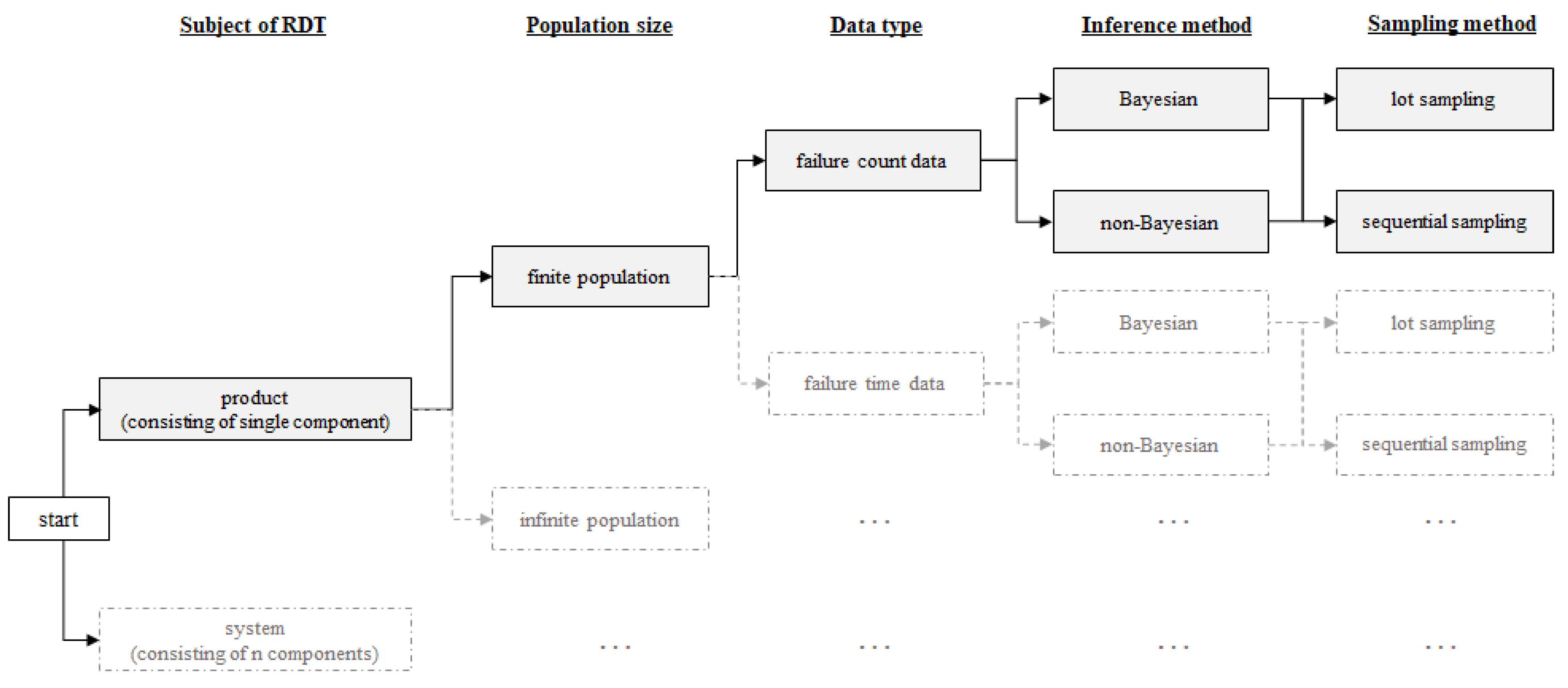
Figure 1 illustrates the scope of the present work, which deals with a finite population of single-component products assessed using failure count data. In order to determine the optimal sample size, lot and sequential sampling are adopted for the RDTs, while the non-Bayesian and Bayesian inference approaches are compared.
Most previous RDT studies calculate the initial sample size n for success-based testing. In this approach, the population is accepted when no defective items are found within a sample of n items. Though success-based testing is regularly employed in industry in the hopes that a sample will contain no defective items and the population will be accepted, defective items are often found during testing due to the fact that the defective ratio q within the population is unknown.
It remains unclear exactly what RDT process should be followed to determine the acceptance of a population when defective items appear in a sample. It is thus necessary to develop an RDT process that has a suitable method for determining the number of additional items from the population that need to be sampled when a defective item appears during testing, while simultaneously considering specific sampling methods, such as lot or sequential sampling. It is particularly important to consider both lot and sequential sampling, because a sufficient sample size for RDTs cannot be guaranteed in new product development projects.
One technical aspect of note in the present work is that the sampling results are immediately used to obtain a posterior distribution from the prior distribution of the population’s parameters using the Bayesian approach. Using the natural-conjugate prior distribution of the likelihood function allows the posterior distribution’s functional form to be expressed easily.
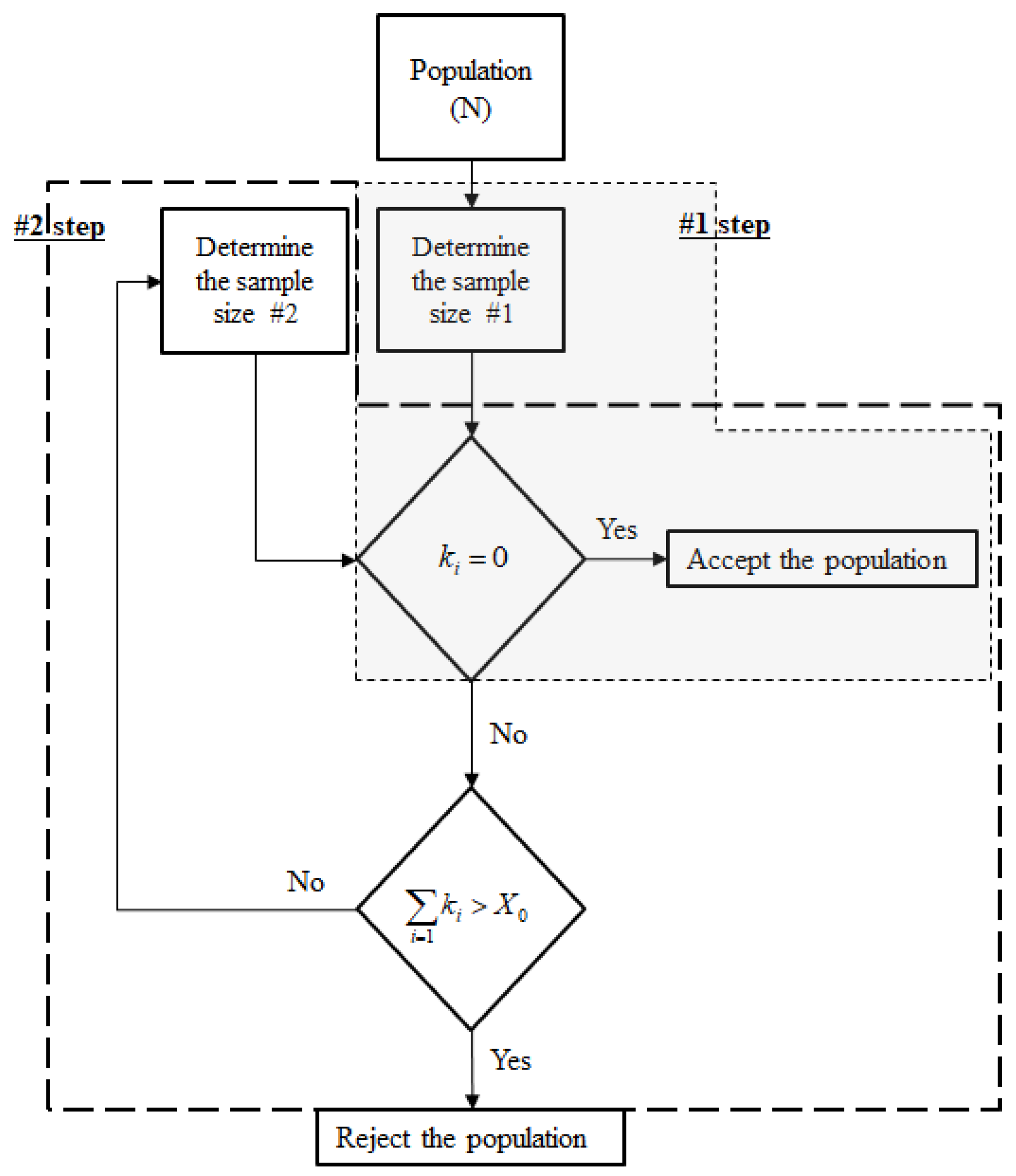
Starting with a population of size N with X defective items within the population, the population size and the number of defective items will be updated after the sampling process in the following manner: and , where is the i-th sample and is the number of defective items in . Figure 2 presents the proposed RDT process for calculating the additional number of items that need to be sampled after detecting defective items during success-based testing.
Whether the population is finite or infinite, and whether prior information is present or absent, are established in the “Population” step. In the “#1 step,” the initial sample size n is determined using the non-Bayesian or Bayesian approach, as explained in Section 3 and Section 4. This initial sample size is calculated using information on population size, confidence level, population reliability, and the inference method without test data. An RDT is then conducted with initial sample size n. The population is accepted when no defects are detected in the initial sample. If the number of defective items k in the initial sample is not 0, the “#2 step” is implemented, in which the value of (e.g., the first sample size n, the second sample size n) can be obtained from N and the maximum number of allowable defective items using both non-Bayesian and Bayesian approaches. If the accumulated number of defects k in the sample exceeds , the population is rejected. The n calculated in the “#2 step” can vary according to the sampling method (i.e., lot or sequential). Therefore, the optimal sample size required for RDTs depends on the sampling method, so both lot and sequential sampling must be considered when determining the sampling size.
4. Sampling Distributions for a Finite Population
The present work employs an RDT for a finite population, and non-Bayesian and Bayesian approaches to determine the optimal sample size. When sampling from a finite population, the size of the population N and the number of defective items X in that population can be written as and , respectively, where is the i-th sample and is the number of defective items in . A Bayesian approach can be used to calculate when conducting an RDT for a finite population. In this approach, the multiplication of the prior distribution and the likelihood function is proportional to the posterior distribution , as expressed in Equation (1):
A binomial probability distribution can be employed under the assumption that either the size of the population is infinite or the samples are independent. When the population is finite and the samples are dependent, a hypergeometric probability distribution should be employed. The present work is particularly interested in RDTs for a finite population. Thus, represents the probability distribution of the samples from a finite population and is expressed as a hypergeometric distribution in Equation (2):
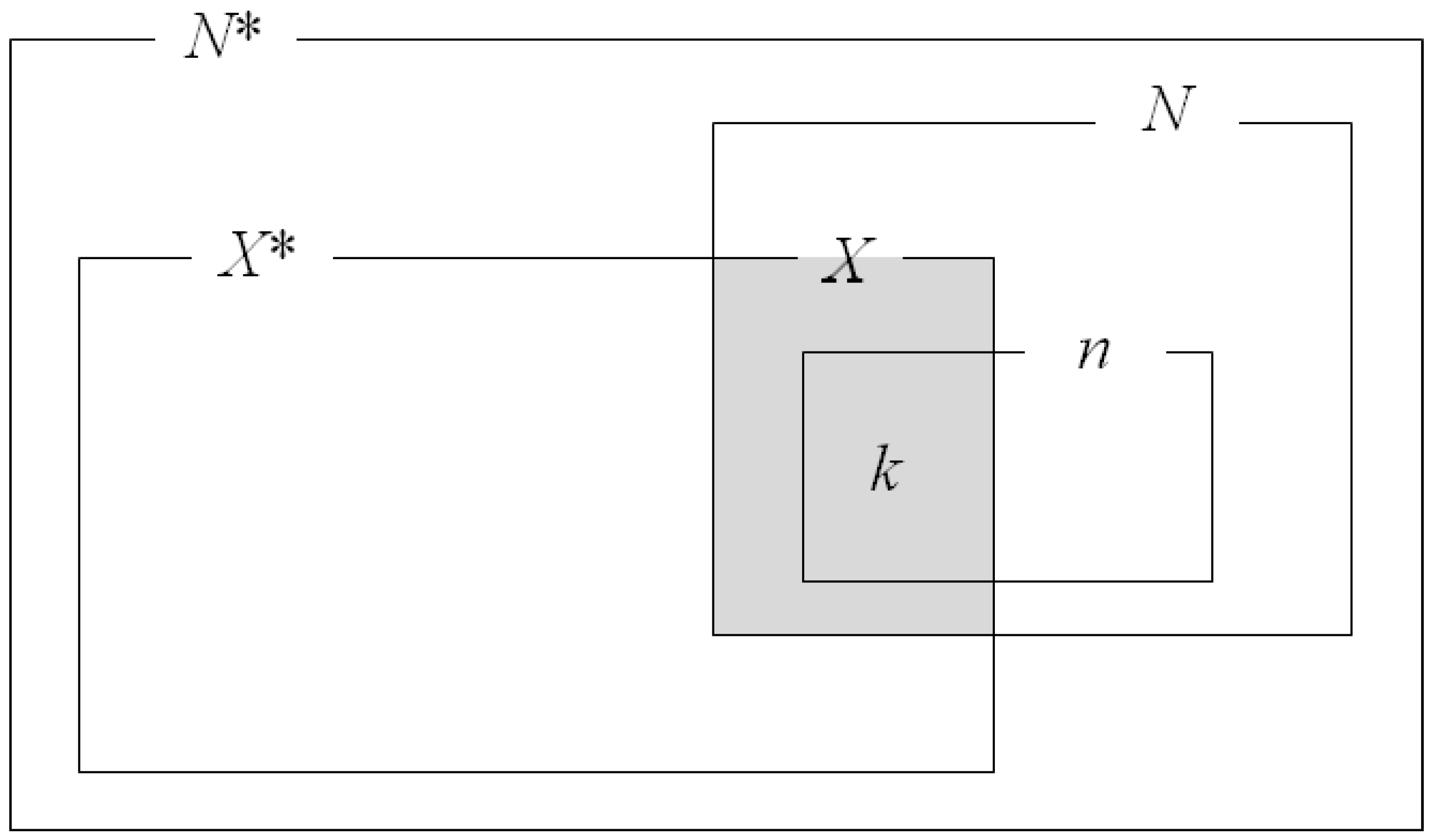
This work mathematically calculates the conjugacy between the hypergeometric distribution and the beta-binomial distribution, and then determines the optimal sample size. The prior distribution is calculated to estimate the posterior distribution . It is reasonable to expect that this can be obtained from the relationship between the sample and population sizes, as illustrated in Figure 3, given the of a large population regarded to be infinite, the N of a finite population, (the total number of defective items in ), X (the number of defects in N), and k (the number of defective items in the sample n). The finite population is assumed be a subset of the infinite population.
The conjugacy between the hypergeometric and beta-binomial distributions is calculated using the first sample (i = 1), as shown in Appendix A [26]. The conjugacy is then verified for i = 2, 3, 4 … through the sequential calculation of the posterior distribution. The generalizations of Equations (A6) and (2) correspond to Equations (3) and (4), respectively, where denotes the number of defective items from .
Combining Equations (A7), (3), and (4) leads to a generalized formula for the i-th posterior distribution, shown in Equation (5):
5. Sample Size Based on the Proposed RDT
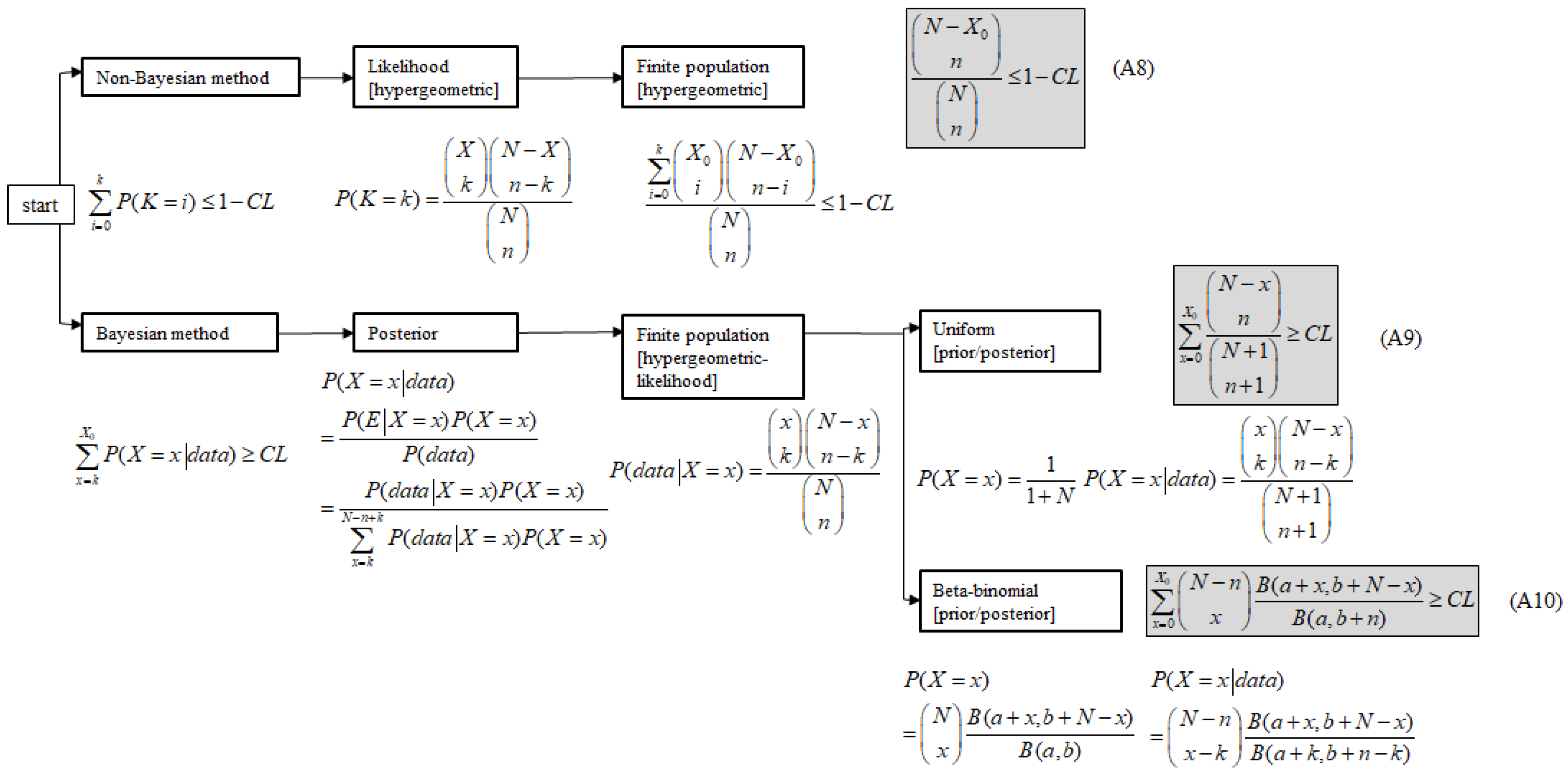
Figure 4 presents the process adopted by the present work to determine the optimal sample size. is the maximum number of allowable defective items, and the initial sample size n is obtained from success-based testing (at k = 0) through a series of calculations using a finite population and the R-C measure.
As shown in Table 1, a population is accepted with 95% reliability and a 90% confidence level for the non-Bayesian approach, when 37 items selected from that population are found to be free of defects. It should be noted that, in the absence of prior information regarding the parameter values for the beta-binomial distribution, it is assumed that a = 1 and b = 1 [10].
Table 1 summarizes the series of calculations used to determine optimal sample size in the RDT process, given N = 100, 95% reliability, and a 90% confidence level target requirement. Here, “Initial n” represents the optimal sample size for success-based testing in the absence of sample data. “First n” in Table 1 is the number of additional items that are required for testing when the initial n contains a defective item. The computation of the optimal sample size is outlined in Appendix B. The value of the initial n differs, depending on which inference method is used to determine the sample size (i.e., non-Bayesian or Bayesian). Once the initial n has been calculated, different sampling methods produce different values for the first n.
Numerical examples show that a beta-binomial Bayesian approach with sequential sampling has the advantage of requiring only a small sample size when determining the acceptance of a finite population. When the beta-binomial Bayesian method is applied, the total number of additional items required for sampling is the same for both lot and sequential sampling, when determining the acceptance or rejection of a finite population. However, the sample size calculated for sequential sampling was the same as or smaller than that obtained for lot sampling because lot sampling tests lots of size n simultaneously, and sequential sampling tests one item at a time.
6. Conclusions
The present work proposed an RDT process that is able to reflect the specific test environment, including the test target, sample size, inference method, and sampling method. Both lot and sequential sampling were considered in this RDT process because optimal sample sizes for RDTs cannot be guaranteed in test environments for new product development projects. This process was implemented when a defective item appeared during success-based testing, employing both non-Bayesian and Bayesian approaches based on R-C failure data for one-shot devices. This work considered the samples to not be independent. Thus, a hypergeometric distribution was adopted as a likelihood function for a finite population consisting of one-shot devices. Based on the Bayesian framework, the conjugacy between the hypergeometric likelihood function and a beta-binomial distribution was mathematically calculated. The posterior beta-binomial distribution was used to decide in the RDT, on whether to accept or reject the population.
The results indicated that a beta-binomial Bayesian approach with sequential sampling has the smallest optimal sample size when determining the acceptance or rejection of a finite population. The proposed RDT process can thus be used in similar test environments, such as in new product development projects.
The present work was founded on the absence of prior information about the target population. In future research, this RDT process could be extended to examine additional ways to decrease the sample size required for RDTs. One possible option in this respect could be changing the parameter values for the prior distribution based on prior information or expert opinion on the population.
Author Contributions
J.J. and S.A. conceived and designed the research; J.J. conducted the research and drafted the manuscript. S.A. supervised the overall work. All authors read and approved the final manuscript.
Funding
This work was supported by the National Research Foundation of Korea (NRF) grant funded by the Korea government (MSIP) (No. NRF-2018R1A2B6003232). This work was supported by the National Research Foundation of Korea (NRF) grant funded by the Korea government (MSIP) (No. NRF-2018R1A2B6003232).
Conflicts of Interest
The authors declare no conflicts of interest.
Appendix A
In this Appendix A, the prior distribution is calculated to estimate the posterior distribution . Given the assumption that the values are close to unlimited, the defective ratio is expressed as (or ). The conditional probability of X given q from N is expressed as in Equation (A1). can be written as in Equation (A2), and denotes the unconditional probability distribution. Combining Equations (A1) and (A2), Equation (A3) can be expressed as in Equation (A4).
The replacement of N with n and x with k in Equation (A4) can be expressed as Equation (A5):
Using Bayes’ theorem, the value of the posterior distribution can be expressed as Equation (A6):
Based on Equations (2), (A4), and (A5), the form of the posterior distribution is identical to that of the beta-binomial distribution, given that k is the number of defective items in a sample. In other words, the parameters for the prior distribution and posterior distribution are updated from and , respectively. The foregoing shows the conjugacy between the hypergeometric distribution and the beta-binomial distribution in Equation (A7):
Appendix B
Appendix B describes the calculation process and equations used to compute the results of Table 1. The non-Bayesian method uses Equation (A8) and the Bayesian method uses Equations (A9) and (A10), to calculate the optimal sample required for RDT. Table 1 shows some of the simulated data assuming defective items were found in the initial samples. Using Equations (A8)–(A10) and the proposed RDT process, we can calculate the optimal n in RDT under different conditions.
As a numerical example, for a population size of N = 100 with 95% reliability (R) and a 90% confidence level (CL), the initial n was calculated to be 37 and 31 for the non-Bayesian (using Equation (A8)) and Bayesian (by using Equations (A9) and (A10)) approaches, respectively, in success-based testing (k = 0). Based on Equation (A8), the optimal sample sizes (n = 37) required for the success-based testing of a population size of N = 100 (R = 0.95, CL = 0.9) are given in Table 1.
When adopting a sequential sampling approach, if the first defective item is the 23rd item of the initial sample (either 37 or 31), is updated with n = 23 and k = 1.
Based on Equations (A8) and (A9), the optimal sample sizes (first n = 34 and first n = 28) required for the success-based testing of the population (R = 0.95, CL = 0.9) are given in Table 1. The value n = 28 is based on a Bayesian uniform distribution. Using the Bayesian beta-binomial distribution Equation (A10), n = 27 is calculated when a = 1 + k and b = 1 + n – k, using n = 23 and k = 1.
The second n in Table 1 is the number of additional items that require testing based on the first n when a second defective item is drawn from the population, whilst the third n represents the number of additional items required for testing based on the second n when a third defective item is drawn from the population. The total n is the overall sample size required for the RDT. The mean and variation of the beta-binomial distribution are Equations (A11) and (A12). The summary statistics of the posterior distribution can be calculated using Equations (A11) and (A12).
Table A1 summarizes the sensitivity of the hyperparameters from a beta-binomial distribution, in the series of calculations used to determine sample size, given N = 100, 95% reliability, and a 90% confidence level target requirement. The larger the value of hyperparameter b, the smaller the initial n.

Table A1.
The sensitivity of the hyperparameters from a beta-binomial distribution.
| a | 1 | 1 | 1 | 1 | 1 |
| b | 1 | 2 | 3 | 4 | 5 |
| Initial n | 31 | 30 | 30 | 29 | 28 |
References
- Hallstedt, S.; Ny, H.; Robèrt, K.; Broman, G. An approach to assessing sustainability integration in strategic decision systems for product development. J. Clean. Prod. 2018, 18, 703–712. [Google Scholar] [CrossRef]
- Michelon, G.; Boesso, G.; Kumar, K. Examining the link between strategic corporate social responsibility and company performance: An analysis of the best corporate citizens. Corp. Soc. Responsib. Environ. Manag. 2013, 20, 81–94. [Google Scholar] [CrossRef]
- Siva, V.; Ida, G.; Árni, H. Organising Sustainability Competencies through Quality Management: Integration or Specialisation. Sustainability 2018, 10, 1326. [Google Scholar] [CrossRef]
- Min, H.; Zhou, G. Supply chain modeling: Past, present and future. Comput. Ind. Eng. 2002, 43, 231–249. [Google Scholar] [CrossRef]
- Li, M.; Zhang, W.; Hu, Q.; Guo, H.; Liu, J. Design and risk evaluation of reliability demonstration test for hierarchical systems with multilevel information aggregation. IEEE Trans. Reliab. 2017, 66, 135–147. [Google Scholar] [CrossRef]
- Xu, J.Y.; Yu, D.; Xie, M.; Hu, Q.P. An approach for reliability demonstration test based on power-law growth model. Int. J. Qual. Reliab. Eng. 2017, 33, 1719–1730. [Google Scholar] [CrossRef]
- National Research Council. Reliability Growth: Enhancing System Reliability; The National Academies Press: Washington, DC, USA, 2015. [Google Scholar]
- Yadav, O.P.; Singh, N.; Goel, P.S.; Itabashi-Campbell, R. A framework for reliability prediction during product development process incorporating engineering judgments. Qual. Eng. 2003, 15, 649–662. [Google Scholar] [CrossRef]
- Ke, H.Y. A Bayesian/classical approach to reliability demonstration. Qual. Eng. 2000, 12, 365–370. [Google Scholar] [CrossRef]
- Lu, M.-W.; Rudy, R.J. Reliability demonstration test for a finite population. Int. J. Qual. Reliab. Eng. 2001, 17, 33–38. [Google Scholar] [CrossRef]
- Kleyner, A.; Elmore, D.; Boukai, B. A Bayesian approach to determine test sample size requirements for reliability demonstration retesting after product design change. Qual. Eng. 2015, 27, 289–295. [Google Scholar] [CrossRef]
- O’Connor, P.; Kleyner, A. Practical Reliability Engineering, 5th ed.; John Wiley & Sons: Chichester, UK, 2012. [Google Scholar]
- Kleyner, A.; Bhagath, S.; Gasparini, M.; Robinson, J.; Bender, M. Bayesian techniques to reduce the sample size in automotive electronics attribute testing. Microelectron. Reliab. 1997, 37, 879–883. [Google Scholar] [CrossRef]
- Chen, S.; Lu, L.; Li, M. Multi-state reliability demonstration tests. Qual. Eng. 2017, 29, 431–445. [Google Scholar] [CrossRef]
- Guo, H. Designing reliability demonstration tests for one-shot systems under zero component failures. IEEE Trans. Reliab. 2011, 60, 286–294. [Google Scholar] [CrossRef]
- Guo, H.; Liao, H. Methods of reliability demonstration testing and their relationships. IEEE Trans. Reliab. 2012, 61, 231–237. [Google Scholar] [CrossRef]
- Guo, H.; Jiang, M.; Wang, W. A method for reliability allocation with confidence level. In Proceedings of the 2014 Annual Reliability and Maintainability Symposium (RAMS), Colorado Springs, CO, USA, 27–30 January 2014. [Google Scholar]
- Jensen, W.A. Binomial reliability demonstration tests with dependent data. Qual. Eng. 2015, 27, 253–266. [Google Scholar] [CrossRef]
- Lu, L.; Li, M. Multiple objective optimization in reliability demonstration Tests. J. Qual. Technol. 2016, 48, 326–342. [Google Scholar] [CrossRef]
- Migon, H.S.; Dani, G.; Francisco, L. Statistical Inference: An Integrated Approach; CRC Press: London, UK, 2014. [Google Scholar]
- Quigley, J.; Bedford, T.; Walls, L. Empirical Bayes estimates of development reliability for one shot devices. Saf. Reliab. 2009, 29, 35–46. [Google Scholar] [CrossRef]
- Ahn, S.E.; Park, C.S.; Kim, H.M. Hazard rate estimation of a mixture model with censored lifetimes. Stoch. Environ. Res. Risk Assess. 2007, 21, 711–716. [Google Scholar] [CrossRef]
- Ahn, S.; Kim, W. Service level analysis of (S-1, S) inventory policy for negative binomial distributed failures. Asia-Pac. J. Oper. Res. 2008, 25, 827–835. [Google Scholar] [CrossRef]
- Guérin, F.; Dumon, B.; Usureau, E. Reliability estimation by Bayesian method: Definition of prior distribution using dependability study. Reliab. Eng. Syst. Saf. 2003, 82, 299–306. [Google Scholar] [CrossRef]
- Percy, D.F. Subjective priors for maintenance models. J. Qual. Maint. Eng. 2004, 10, 221–227. [Google Scholar] [CrossRef]
- Richard, E.B. Engineering Reliability; Society for Industrial and Applied Mathematics (SIAM): Philadelphia, PA, USA, 1998; Volume 2. [Google Scholar]
Figure 1.
Scope of the current work.

Figure 2.
The proposed reliability demonstration test (RDT) process.

Figure 3.
Relationship between the sample and population sizes.

Figure 4.
Classification of non-Bayesian and Bayesian methods for the determination of sample size.

Table 1.
Results for the n values by method (95% reliability and 90% confidence level).
| Method | Prior | Sampling | Initial n | First n | Second n | Third n |
|---|---|---|---|---|---|---|
| Non-Bayesian | no prior | lot | 37 | 27 (total 64) | 19 (total 83) | 12 (total 95) |
| sequential | 37 | 34 (total 57) (failure at 23rd item) | 28 (total 76) (failure at 48th item) | 27 (total 87) (failure at 60th item) | ||
| Bayesian | uniform | lot | 31 | 25 (total 56) | 19 (total 75) | 13 (total 88) |
| sequential | 31 | 28 (total 51) (failure at 23rd item) | 22 (total 70) (failure at 48th item) | 21 (total 81) (failure at 60th item) | ||
| beta-binomial | lot | 31 | 19 (total 50) | 16 (total 66) | 13 (total 79) | |
| sequential | 31 | 27 (total 50) (failure at 23rd item) | 18 (total 66) (failure at 48th item) | 19 (total 79) (failure at 60th item) |
© 2018 by the authors. Licensee MDPI, Basel, Switzerland. This article is an open access article distributed under the terms and conditions of the Creative Commons Attribution (CC BY) license (http://creativecommons.org/licenses/by/4.0/).
Share and Cite
MDPI and ACS Style
Jeon, J.; Ahn, S. Bayesian Methods for Reliability Demonstration Test for Finite Population Using Lot and Sequential Sampling. Sustainability 2018, 10, 3671. https://doi.org/10.3390/su10103671
AMA Style
Jeon J, Ahn S. Bayesian Methods for Reliability Demonstration Test for Finite Population Using Lot and Sequential Sampling. Sustainability. 2018; 10(10):3671. https://doi.org/10.3390/su10103671
Chicago/Turabian StyleJeon, Jongseon, and Suneung Ahn. 2018. "Bayesian Methods for Reliability Demonstration Test for Finite Population Using Lot and Sequential Sampling" Sustainability 10, no. 10: 3671. https://doi.org/10.3390/su10103671
Note that from the first issue of 2016, this journal uses article numbers instead of page numbers. See further details here.