Measuring the Macroeconomic Performance among Developed Countries and Asian Developing Countries: Past, Present, and Future

Abstract

The purpose of this paper is to measure and forecast the macroeconomic performance in developed countries and Asian developing countries over the periods from 2013 to 2016 and 2017 to 2020. We used four macroeconomic indicators: government gross debt, real GDP growth, inflation rate, and unemployment rate to construct a scalar-valued summary measure of macroeconomic performance. These indicators are inspired by data envelopment analysis (DEA)-based models, which allow for unequal weighting of the different economic objectives. Based on the resampling models of DEA, we developed a research procedure for solving the macroeconomic performance problem by integrating gauge and forecast. Two variants of resampling models of DEA, i.e., past-present and past-present-future, were used to gauge and forecast the relative performance for each country in each year. Throughout the analysis, emphasis is placed on a comparison of the performances of 12 Asian developing countries with those of the five developed countries. Our empirical results reveal that Switzerland, Singapore, and the United States have achieved the most successful macroeconomic management in a time-series.

1. Introduction

The stability of a macroeconomic environment plays an important role for business and, therefore, has significance for the overall competitiveness of a country. Although it is certainly true that macroeconomic stability alone cannot increase the productivity of a nation, it is also recognized that macroeconomic disarray harms the economy [1]. As we have seen over the past years in the European community, a government cannot provide services efficiently if it has to make high interest payments on its past debts. Furthermore, firms cannot operate efficiently when inflation rates are out of hand. In summary, the economy cannot grow in a sustainable manner unless the macro environment is stable. Each economy has an apparatus responsible for the conduct of its macroeconomic policy, i.e., the helmsman [2]. Initially, the helmsmen are assumed to provide varying amounts of macroeconomic services. Some macroeconomic services include a high level of real GDP per capita, a low rate of inflation, a high employment rate, a favorable trade balance, and so on. Thus, macroeconomic performance is evaluated in terms of the ability of the helmsmen in each country to maximize provision of these fundamental macroeconomic services.

Various contributions in the past have measured macroeconomic performance using different approach. First is Okun’s misery index [3]. The Okun index of a nation is defined as the sum of both its unemployment rate and inflation rate. The Calmfors–Driffill index was developed by Calmfors and Driffill [4]. The measure is obtained as the sum of unemployment rate and trade balance normalized by its gross national product. Both these measures give useful information but still flawed. The Okun and Calmfors–Driffill index are obtained by using two single indicators (unemployment rate, inflation rate and the sum of unemployment rate, trade balance) and both attach equal unitary weights to their respective components. The OECD’s “magic diamond” is rebased on four macroparameters such as GDP growth, trade balance, inflation, and unemployment, but also attaches equal unitary weights to its components. The implicit assumption that policymakers assess all policy goals equally important, or, in other words, that no priorities are attributed. This seems an unrealistic hypothesis. Equality across components is unnecessarily because they depend each countries’ different objective through time. That means that sometimes a lower value is again associated with better macroeconomic performance, and whenever there is need for a change in policy priorities, the policymakers face tradeoffs among these objectives. So, the main shortcoming of these gauges is the arbitrary weighting scheme they share. Therefore, it is imperative to seek a scientific methodology that helps one to determine unequal weights for macro indicators, which the weight of each indicator reflecting the policy priority assumed by the policy-makers. The emergence of DEA well suited to obtain such synthetic indicators. It allows for a ranking of economies on the basic of their relative performance.

The DEA was introduced by Charnes et al. [5]. They proposed a “data oriented” approach for measuring the performance of multiple decision-making units (DMUs) by converting multiple inputs into outputs. DMU could include schools, universities, bank, hospitals, power plants, etc. In the past few years, some researchers have implemented the DEA approach to measure environmental, energy, and economic performance in economies and regions. Wang et al. used data envelopment analysis and the heuristic technique approach to help department stores find the most suitable partners for strategic alliances [6]. Yuan and Tian applied the DEA model to analyze the science and technology resources efficiency of industrial enterprises. The results reflected the independence of the input element and the concentration of the output element [7]. Wu et al. assessed the industrial energy efficiency with CO₂ emissions in China by means of DEA [8]. Egilmez et al. employed DEA to analyze the sustainability performance and improve the energy efficiency of the U.S. manufacturing sector [9]. Chang used the DEA model and directional distance function model to measure the overall efficiency of G7 and BRICS countries. The study found out that G7 countries have higher efficiency than BRICS countries before 2005 [10].

Some other researchers have implemented the DEA approach to measure macroeconomic performance (MEP) of economies. For instance, Lovell [11] used mathematical programming techniques of efficiency measurement to construct a “best practice” macroeconomic performance frontier, and then to measure performance in terms of an indicator-based efficiency score. The paper is applied to 10 Asian economies, with special attention paid to Taiwan in the period 1970 to 1988. Lovell et al. [12] studied the macroeconomic performance of 17 OECD countries over the period from 1970 to 1990 using data envelopment analysis (DEA). Cherchye [13] used a DEA-based model, which allowed for unequal weighting of the different economic objectives. The study provided a comparison of several synthetic indicators that merged four separate indicators into a single statistic. Despite the similarity of the research model, the results of the previous studies had differences. To be specific, Lovell [11] established a scalar-valued measure of the macroeconomic performance of an economy. However, in this application there are no inputs and only contains four outputs (GDP growth, employment, trade balance, and price stability). Moreover, the study was conducted in a small scale of 10 economies in Asian for varying lengths of time, it was difficult to come up with a convincing overall performance ranking. Or Cherchye [13] who provided a comparison of several synthetic indicators that merged four separate indicators into one single statistic to evaluate 20 OECD countries for four years. Our study has produced outstanding results when selecting four indicators (government’s gross debt, real GDP growth, inflation rate, and unemployment rate) as inputs/outputs. Of which, the government gross debt indicator is replaced by the trade balance indicator of Lovell [11]. Data was collected from 17 economies show the big picture of macroeconomic.

Notably, unlike in the earlier convergence study, the highlight of the current study is predicting macroeconomic performance based on historical data using new resampling models in the DEA approach. A traditional DEA model is known as a measure of the effectiveness of DMUs based on past data. In this model, Tone and Ouenniche [14] proposed two resampling models, in which the first model utilizes historical data, e.g., past-present, for estimating data variations, imposing chronological order weights that are supplied by the Lucas series. The second model deals with future prospects that aims at forecasting the future efficiency score and its confidence interval for each DMU. By combining with the super-SBM model, none of the past studies were able to provide a comprehensive picture from the past, present, and future concerning macroeconomic performance. Therefore, this present study is considered the first of its kind in assessing and forecasting the relative performance of Asian developing economies by simultaneously considering all the macro indicators; at the same time, it helps one to see the overall picture of global macroeconomic performance.

One of the contributions of this study uses of the resampling model, i.e., a new DEA model included in our research. Resampling models are new models developed by Tone and Ouenniche in 2016 [14]. In this model, Tone and Ouenniche proposed new resampling models, based on these variations, for gauging the confidence intervals of DEA scores. The first model utilizes past-present data for estimating data variations imposing chronological order weights that are supplied by the Lucas series. The second model deals with future prospects. This model aims at forecasting the future efficiency score and its confidence interval for each DMU.

The goal of this study is to combine the popular super-SBM model in DEA with two new models in resampling to build “a model combining assessment and forecasting of macroeconomic performance” from past, present, and future. To the best of our knowledge, no previous research has done this; not only is this new to the field of macroeconomic performance, but it can be applied to other research subjects.

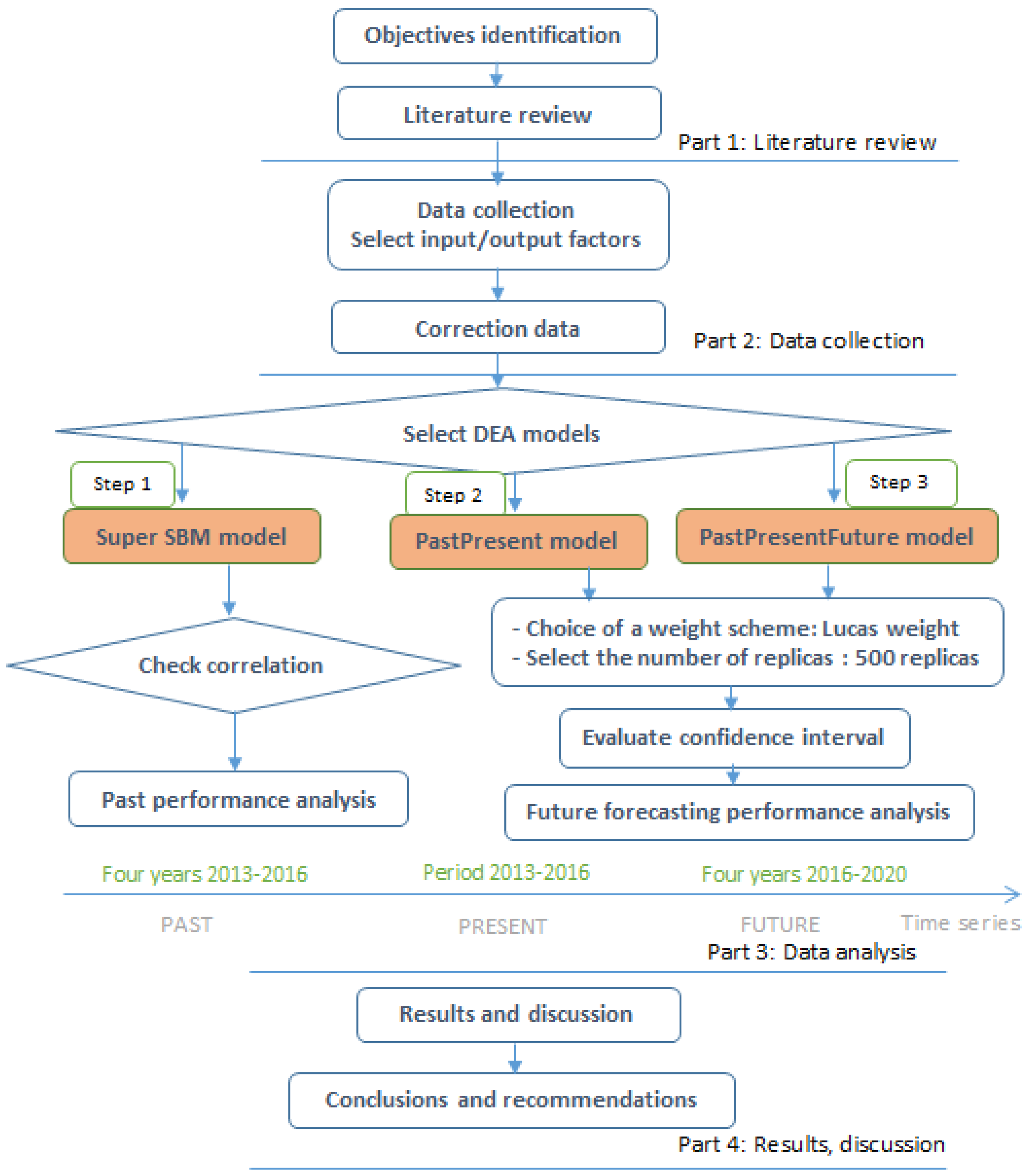
In this paper, we integrate DEA models to gauge and forecast the relative performance of economies, in which the authors applied the super-SBM model and the past-present model to combine ranking and evaluating performance year by year for the period of 2014 to 2016. Then, the authors used two resampling models, i.e., past-present and past-present-future, to evaluate and forecast the next years for the period of 2017 to 2019. In this study, Lucas weights were used for past and present data, selecting 500 replicas, and evaluating confidence intervals before performance analysis. The study was divided into five parts, as shown in Figure 1.

2. Materials and Methods

2.1. Macroeconomic Data

Each country has an apparatus responsible for conducting its macroeconomic policy. Although the size and organizational structure of this bureaucracy vary across countries, through time, the authors view such variation as irrelevant to the objective of research. What matters is its macroeconomic performance. All data used in the analysis are taken from various International Monetary Fund (IME) publications and the World Bank. Data for the labor capital indicator are taken from the World Bank [15], while the five remaining indicators are taken from annual issues of the IMF’s World Economic Outlook, Balance of Payments Statistics, and International Financial Statistics [16]. Due to data availability of Asian developing countries, this study takes the data of 12 economies in the area as a sample. Moreover, the authors added five countries with the highest global competitiveness index (GCI) in the world for analysis. This makes it more abundant to compare the effectiveness of macroeconomic policies. All data cover 17 countries over the period from 2013 to 2016.

The authors follow the principles stated in Cook, Tone, and Zhu [17] in this study and believe that DEA performance measures are relative, not absolute, and frontier-dependent. The use of inputs and outputs are proportionate to the number of DMUs. The variables selected to reflect the macroeconomic performance of the economies are as follows:

1. Government gross debt: Government’s gross debt to GDP ratio is the amount of a country’s total gross government debt as a percentage of its GDP. It is an indicator of an economy’s health and a key factor for the sustainability of government finance [16].

2. Real GDP growth: Gross domestic product is the most commonly used single measure of a country’s overall economic activity.

3. Inflation rate: Inflation is a sustained increase in the general price levels of goods and services in an economy over a period of time. Inflation reflects a reduction in the purchasing power per unit of money of an economy [18]. Inflation is defined as the rate of percent change in the consumer price index (PCI) [16].

4. Unemployment rate: Number of employed persons as a percentage of the total labor force. Employment rate is defined (E/L)_t, i.e., the ratio of civilian employment (E) to the civilian labor force (L). Employment rate in the longer term is significantly affected by a government’s policies [19].

Because a government’s gross debt, inflation rate, and unemployment rate are undesirable factors, we convert them to a measure of “uninflation”, “employment”, and “government gross debt”. The indicators of real GDP growth, employment rate, and price stability each take on strictly positive values for all observations. General government gross debt takes on negative values for some observations, and DEA is not capable of dealing with negative values. Consequently, general government gross debt has been transformed to a (0–100) scale prior to analysis. Variable transformations are given by [11] transformed output = α + β (raw output), where α = 100(min/(max − min), β = 100/(max − min).

Table 1. Main statistics of inputs/outputs for 17 countries (average, 2013–2016).

Variable	(I) GGB	(I) R-GDP	(O) I-Rate	(O) U-Rate	(I) GGB	(I) R-GDP	(O) I-Rate	(O) U-Rate
2013					2014
Max	99.04671	7.8	100.2	99.7	99.80952	7.3	100	99.9
Min	0.005	0.6	93.4	92	0.002	0.9	93.6	92.1
Average	52.62184	3.717647	97.45294	95.53529	52.62197	3.905882	97.64118	95.80588
SD	25.94456	2.23218	1.762724	2.327064	25.38443	1.874432	1.688737	2.156923
	2015				2016
Max	99.80971	7.2	101.1	99.8	99.82047	7	100.5	99.7
Min	0.002	1.2	93.6	92.6	0.002	1.4	96.5	93
Average	51.8387	3.782353	99	95.91765	53.87064	3.641176	98.62353	95.92353
SD	25.55768	1.920856	1.692544	1.959062	25.07653	1.936965	1.132166	1.893186

shows a summary of statistics for input and output factors for selected countries between 2013–2016. The paper points out government gross debt, real GDP growth, the inflation rate, and unemployment rate of 17 economies.

2.2. Methodology

2.2.1. Resampling model in DEA

In principle one might choose from a relatively wide range of DEA models. However, Tone and Ouenniche [14] recommended the use of the non-oriented super slacks-based measure model (previously called the super-SBM model) [20] under the constant returns-to-scale (CRS) assumption for evaluating the relative efficiency. This model was an extension of the SBM [21].

2.2.2. Historical Data Model (Past-Present Based Framework)

Historical data (previously called past-present information): Let the historical set of the input and output matrix be (X^t, Y^t) (t = 1, …, T). where t = 1 is the first period and t = T is the last period with $X^t=(x_1^t,\dots x_n^t)$ and $Y^t=(y_1^t,\dots y_n^t)$. The number of the DMU is n, and $x_j^t\in R^m$ and $y_j^t\in R^s$are the input and output vectors of DMU_j, respectively.

Choice of a weighting scheme for historical data: Tone and Ouenniche [14] used Lucas weight to weight information on the past and the present. By setting the weight w_t to period t and assuming the weight is increasing in t. For this purpose, the following Lucas number series (l₁, …, l_T) (a variant of Fibonacci series) was a candidate where we had

l_t+2 = l_t + l_t+1 (t = 1, …, T, T − 2; l₁ = 1, l₂ = 2)

(1)

Let the sum be $L={\displaystyle \sum _{t=1}^T{l}_t}$ and weight w_t is defined by:

w_t = l_t/L (t = 1, …, T).

(2)

In this paper, we set T = 4, we had w₁ = 0.0909, w₂ = 0.1818, w₃ = 0.2727, and w₄ = 0.4545. Thus, the influence of the past period faded away gradually.

Super-efficiency scores: Tone and Ouenniche [14] used historical data (X^t, Y^t) (t = 1, …, T) to gauge the confidence interval (CI) of the last period’s scores. The super-efficiency scores of the last period’s DMUs were evaluated firstly. Then, DMU’s CI was gauged using replicas from (X^t, Y^t) (t = 1, …, T) as follows.

Choice of the replication process and the number of replicas: The historical data (X^t, Y^t) (t = 1, …, T) was regarded as discrete events with probability w_t and cumulative probability:

$$W_t={\displaystyle \sum _{i=1}^t{w}_i(t=1,\dots ,T)}.$$

(3)

The replication process based on bootstrapping was first proposed by Efron [22]. Bootstrapping refers to a collection of method that randomly resample with replacement for the original sample. Bootstrapping could be either parametric or nonparametric. For a noncorrelated and homoskedastic dataset, one could for example use smooth bootstrapping or Bayesian bootstrapping, where smooth bootstrapping generates replicas by adding small amounts of zero-centered random noise to resampled observations, whereas Bayesian bootstrapping generates replicas by reweighting the initial data set according to a randomly generated weighting scheme.

In this paper, we use a variant of Bayesian bootstrapping whereby the weighting scheme consists of the Lucas number series-based weights w_t presented above, because it is more appropriate when one is resampling over a past-present time frame and more recent information is considered more valuable. For a noncorrelated and homoskedastic dataset, our data generation process (DGP) in this study may be summarized as follows. First, a random number Ϛ is draw from the uniform distribution over the interval [0, 1], the whichever cross section data (X^t, Y^t) so that W_t−1< Ϛ < W_t is resampled, where W₀ = 0. This process is repeated as many times as necessary to produce the required number of valid replicas or samples.

There is no general rule to the choice the number of replicas B except that the larger the value of B the more stable the results [14]. However, we would keep increasing the value of B until the simulation converges. That mean the results from a run do not change when adding more iterations.

Fisher’s z transformation: Computing the correlation coefficient of two inputs (outputs and input vs. output) items of the last period data over the all DMUs. Then, calculating its $\zeta$% confidence interval, e.g., 95%, using Fisher’s z transformation [23,24]. If the corresponding correlation of a resample data was out of range of this interval, we discard this resample data. The same process between all pair of inputs, outputs, and input vs. output were executed. Thus, inappropriate samples with unbalanced inputs and outputs relative to the inputs and outputs of the last period are excluded from resampling. The above noted 95% confidence interval was not compulsory. The narrower the interval, the closer the resample would be to the last period data.

2.2.3. Resampling with Future Forecasting or Past-Present-Future Model

Tone and Ouenniche [14] forecasted “future” (X^t+1, Y^t+1) by using “past-present” data (X^t, Y^t) (t = 1, …, T) and forecast the efficiency scores of the future DMUs with their confidence intervals.

Forecasting future data: Let h^t (t = 1, …, T) be the observed historical data for a certain input/output of a DMU. Wishing to forecast h^T+1 from h^t (t = 1, …, T). There are three scenarios of forecasting engines available for this purpose. First, trend analysis: a simple linear least square regression. Second, weight average: weight by Lucas number. And finally, the average of trend and weight averae. In this study, we chose a Lucas weight analysis scenario to forecast for the problem at hand. By applying the Lucas weight forecasting model, we obtained data set (X^t+1, Y^t+1). Then, we assumed the super-efficiency for the “future” DMU (X^t+1, Y^t+1).

3. Empirical Analysis of Macroeconomic Performance

3.1. Preliminary Results

Table 2. Super-SBM score.

Economies	DMUs	2013	2014	2015	2016	Economies	DMUs	2013	2014	2015	2016
Australia	E1	0.528	0.635	0.717	0.633	Singapore	E10	1.141	0.872	1.107	1.049
Cambodia	E2	0.460	0.544	0.473	0.454	Thailand	E11	0.546	1.753	0.680	0.594
China	E3	0.443	0.528	0.471	0.455	Vietnam	E12	0.499	0.600	0.513	0.504
HK SAR	E4	0.444	0.557	0.658	0.666	Germany	E13	1.664	0.979	0.996	0.788
Indonesia	E5	0.426	0.521	0.490	0.459	Sweden	E14	0.665	0.703	0.572	0.570
Korea, Rep.	E6	0.508	0.622	0.668	0.604	Switzerland	E15	0.584	0.706	1.227	1.150
Malaysia	E7	0.516	0.598	0.557	0.596	U-Kingdom	E16	0.729	0.845	0.880	0.863
New Zealand	E8	0.532	0.632	0.615	0.526	United States	E17	1.082	1.071	1.042	1.135
Philippines	E9	0.441	0.536	0.480	0.429	Avg		0.659	0.747	0.714	0.675

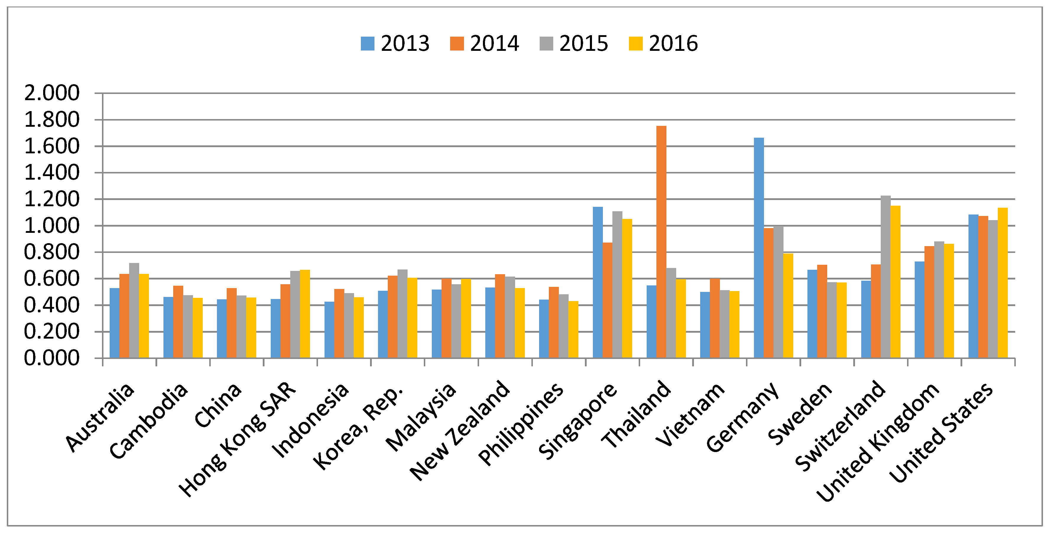
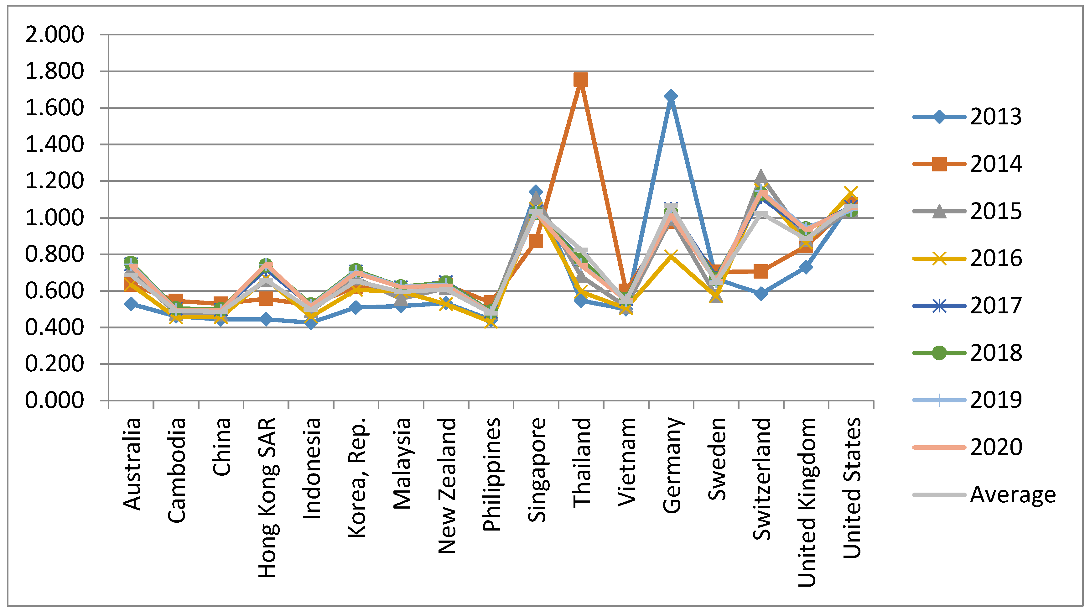
Source: Calculated by researcher.

and Figure 2 show the variation of efficiency scores of economies from 2013 to 2016 and average of four years source-calculated by the researcher. In general, the efficiency scores fluctuated by year. From the results of comparing the averages of four years, we found that the average 0.659 of year 2013 was the lowest score whereas year 2014 had the highest score.

Some economies in Asian developing areas (Cambodia, China, Indonesia, Philippines, and so on) had the lowest efficiency scores and the most invariable efficiency scores in economies which accounted for approximately 5.0. Singapore was the only country in the areas achieving relavitely high performance scores from 1.141 in 2013, 0.0872 in 2014, 1.107 in 2015, and 1.049 in 2016.

Next, some countries such as the United Kingdom, Switzerland, and Germany still had higher scores than the rest. Germany peaked at 1.664 in 2013, fell suddenly in 2014 with a score of 0.979 and remained at 0.996 and 0.788 for 2015 and 2016, respectively. Specially, the United States peaked at 1 for all four years.

Besides, Figure 2 shows the variation between years for each economy. Specicially, Thailand (E11) and Germany (E13) fluctuated dramatically in a positive way at years 2013 and 2014. However, their scores then fell back to approximately average scores in the subsequent years.

3.2. Illustration of the Past-Present Framework

We applied the proposed procedure to the historical data of 17 economies for four years (2013–2016) in Table 1. In this study, we use Lucas weights for past and present data.

Testing replicas and correlation

Table 3. Comparisons of 5000 and 500 replicas (Fisher 95%) period 2013 to 2016.

DMU	5000 Replica			500 Replica			Difference
	97.50%	DEA	2.50%	97.50%	DEA	2.50%	97.50%	2.50%
Australia	0.774	0.633	0.527	0.782	0.633	0.527	−0.0083	−0.0001
Cambodia	0.548	0.454	0.449	0.547	0.454	0.448	0.0002	0.0008
China	0.541	0.455	0.439	0.541	0.455	0.439	−0.0006	−0.0002
Hong Kong SAR	0.764	0.666	0.476	0.762	0.666	0.478	0.0017	−0.0014
Indonesia	0.560	0.459	0.442	0.548	0.459	0.441	0.0129	0.0011
Korea, Rep.	0.721	0.604	0.521	0.713	0.604	0.516	0.0083	0.0051
Malaysia	0.692	0.596	0.502	0.695	0.596	0.500	−0.0023	0.0019
New Zealand	0.745	0.526	0.488	0.745	0.526	0.480	0.0002	0.0074
Philippines	0.531	0.429	0.428	0.530	0.429	0.427	0.0011	0.0009
Singapore	1.171	1.033	0.713	1.172	1.033	0.707	−0.0010	0.0065
Thailand	1.517	0.594	0.543	1.518	0.594	0.545	−0.0011	−0.0013
Vietnam	0.606	0.504	0.486	0.606	0.504	0.488	0.0003	−0.0020
Germany	1.747	0.788	0.788	1.787	0.788	0.788	−0.0403	−0.0005
Sweden	1.091	0.570	0.511	1.232	0.570	0.513	−0.1411	−0.0020
Switzerland	1.403	1.045	0.639	1.376	1.045	0.641	0.0269	−0.0020
United Kingdom	1.064	0.863	0.684	1.066	0.863	0.683	−0.0020	0.0007
United States	1.195	1.135	0.802	1.194	1.135	0.802	0.0013	0.0000

and

Table 4. Lower/upper bounds of Fisher 95% confidence for correlation matrix.

		Lower Bounds
		GGD	Real-GDP	I-Rate	U-Rate
Upper bounds	GGD		−0.1902	−0.7428	−0.5309
	Real-GDP	0.694		−0.8665	−0.2386
	I-rate	0.0905	−0.2649		−0.6114
	U-rate	0.4269	0.6664	0.3243

illustrate the process of constructing replicas and evaluating correlation coefficients for the study results. Meanwhile, Table 3 exhibits the resampling results of 500 and 5000 replicas obtained with a 95% confidence interval. However, the number of replicas depends on the number of inputs, outputs, and DMUs [14]. Hence, we need to check the variations of scores by increasing the number of replicas. In this study, the results from the data analysis show that the difference was negligible. We found 26 out-of-range samples, 500 replicas obtained 0.052%, and 236 out-of-range samples, 5000 replicas obtained 0.047% discards. 500 replicas may be acceptable in this case.

Fisher 95% confidence intervals are shown in Table 4. For instance, the correlation coefficient between government gross debt and unemployment rate is −0.0676 and its 95% lower/upper bounds are −0.5309 and 0.4269, respectively. The correlation coefficient applied the DEA model shows a linear relationship between input and output factors. The correlation coefficient is always between (−1) and (+1), the closer the correlation is to (±1), the closer it is to a perfect linear linear relationship.

The past performance evaluation results

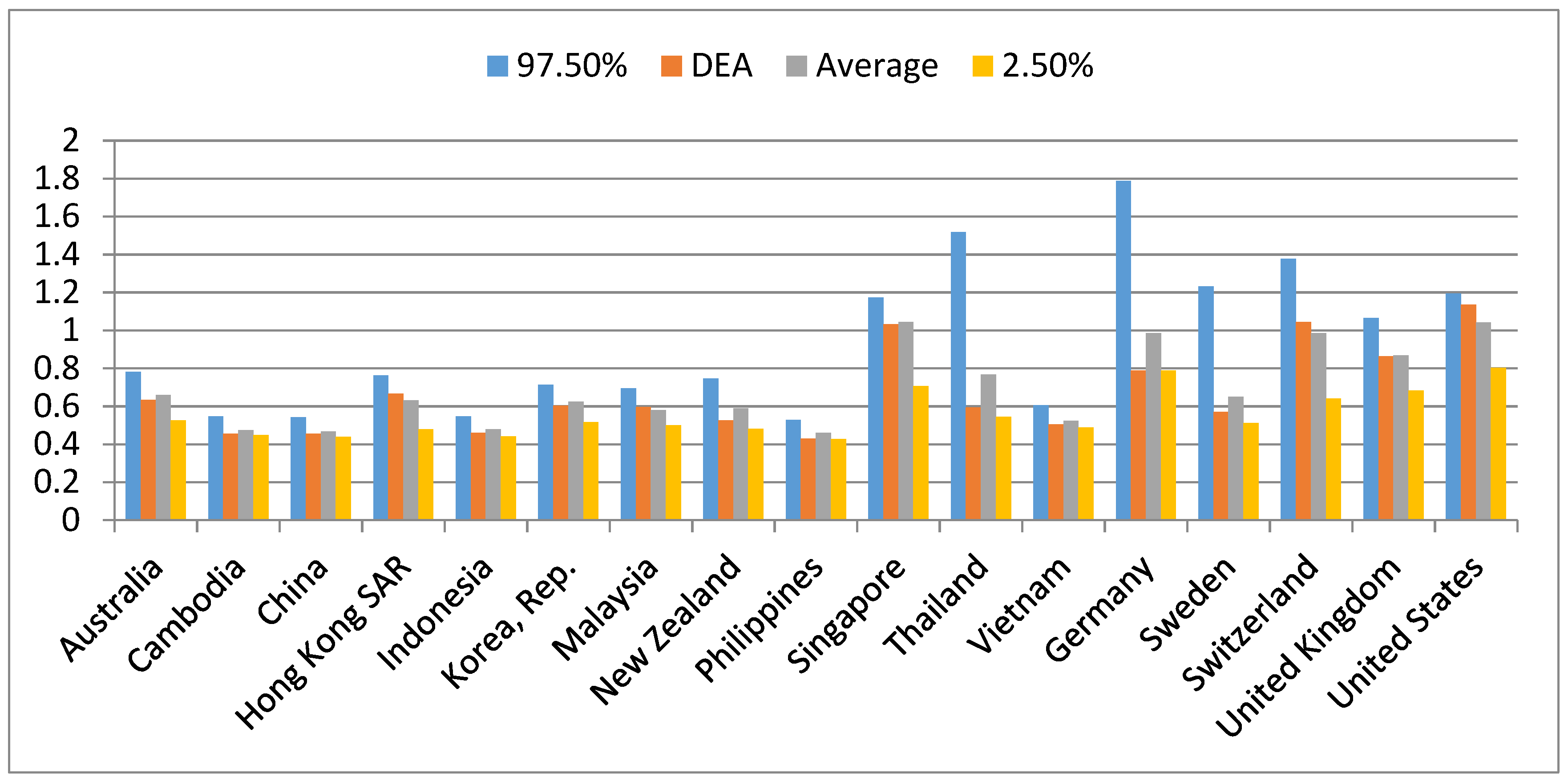
We evaluated the efficiency score of each DMU by using the super-SBM model. To be specific,

Table 5. DEA score and confidence interval with 500 replicas.

DMUs	97.50%	DEA	Avg	2.50%	Rank	DMUs	97.50%	DEA	Avg	2.50%	Rank
E1	0.782	0.633	0.66	0.526	7	E10	1.172	1.033	1.044	0.706	1
E2	0.547	0.454	0.473	0.448	15	E11	1.518	0.594	0.768	0.545	6
E3	0.541	0.455	0.468	0.439	16	E12	0.606	0.504	0.522	0.488	13
E4	0.762	0.666	0.632	0.478	9	E13	1.787	0.788	0.986	0.788	3
E5	0.547	0.459	0.479	0.441	14	E14	1.232	0.569	0.65	0.512	8
E6	0.713	0.604	0.625	0.516	10	E15	1.376	1.045	0.985	0.641	4
E7	0.695	0.596	0.579	0.499	12	E16	1.066	0.863	0.867	0.683	5
E8	0.745	0.526	0.588	0.48	11	E17	1.194	1.135	1.042	0.802	2
E9	0.529	0.429	0.459	0.427	17

Source: Calculated by researcher.

and Figure 3 give information about the DEA score, average score, ranking, and their confidence interval with 500 replicas for the last period, year 2016.

Table 5 exhibits the results obtained by 500 replicas where the column DEA is the last period’s (2016) efficiency score and average indicated the average score over 500 replicas. The column rank is the ranking of average scores. We applied the Fisher 95% threshold and found 26 out-of-range samples.

As can be clearly seen from the given diagram, results fluctuated for each indicator. With DEA score, the number of efficient DMUs is 3, and the number of inefficient DMUs is 14. In fact, three countries, i.e., Singapore, Switzerland, and United States were considered to be highly efficient, Singapore (E10) accounted for 1.033, Switzerland (E15) for 1.045, and United States (E17) for 1.135. The efficiency scores were lower than 0.5 in Cambodia (E2), China (E3), and Indonesia (E5). The other countries’ DEA efficiency scores are between 0.5 and 0.9.

However, ranking with a confidence interval of 97.5% resulted in seven efficient DMUs and 10 inefficient DMUs. Inside, Singapore (E10) still remained the highest raking (the 97.5% confidence interval score was 1.172 and the average score was 1.044), and United States (E17) had the second ranking (the 97.5% confidence interval score was 1.194 and the average score was 1.042). The other 14 countries had efficiency scores which fluctuated between 0.541 for the confidence interval score, 0.454 for the average score, and a ranking between 3 to 16. The Philippines’ performance was deemed to be the worst when ranked at the bottom of the board.

3.3. Illustration of the Past-Present-Future Framework

Hereafter, we present results for the past-present-future framework. In this case, we regard the period from 2013 to 2016 as the past-present and 2017 as the future. We used three simple prediction models to forecast the future, the Trend model, Lucas weights model, and a hybrid model that consists of averaging their predictions with 500 replicas to forecast and examine the future efficiency in 17 economies.

Table 6. 2017 forecasts: Lucas weight, DEA score, and ranking.

Forecast DEA and Confidence Interval						Forecast Data by Lucas Case
DMU	97.50%	DEA	AVG	2.50%	Rank	(I) GGD	(I) R-GDP	(O) I-Rate	(O) U-Rate
Australia	0.783	0.745	0.682	0.533	7	84.05	2.49	98.32	94.12
Cambodia	0.538	0.502	0.48	0.451	15	84.95	7.11	97.33	99.76
China	0.531	0.496	0.475	0.441	16	82.41	6.96	98.11	95.95
HK SAR	0.789	0.719	0.657	0.486	8	99.87	2.35	96.81	96.96
Indonesia	0.552	0.52	0.491	0.447	14	88.81	5.03	94.92	94.12
Korea, Rep.	0.726	0.706	0.647	0.528	10	84.34	2.90	99.00	96.42
Malaysia	0.678	0.619	0.589	0.521	12	72.18	4.79	97.72	96.71
New Zealand	0.735	0.647	0.604	0.492	11	87.70	3.21	99.33	94.70
Philippines	0.524	0.484	0.467	0.431	17	85.01	6.55	97.77	93.90
Singapore	1.152	1.033	1.051	0.813	1	55.68	2.54	99.96	97.99
Thailand	1.416	0.771	0.766	0.559	6	82.15	2.65	99.61	99.18
Vietnam	0.595	0.554	0.531	0.492	13	75.75	6.23	97.26	97.69
Germany	1.775	1.048	0.993	0.795	4	70.35	1.67	99.50	95.45
Sweden	1.128	0.674	0.648	0.521	9	82.10	3.15	99.24	92.64
Switzerland	1.369	1.11	1.002	0.632	3	81.78	1.59	100.50	95.11
United Kingdom	1.041	0.932	0.891	0.727	5	62.90	2.15	99.17	94.50
United States	1.199	1.06	1.042	0.827	2	55.66	2.10	98.95	94.51

(Hong Kong = HK SAR, Government gross debt = GGD; Real GDP growth = R-GDP; Inflation rate = I-rate; Unemployment rate = U-rate). Source: Calculated by researcher.

points out the detailed evaluation results of 2017 for the input/output, forecast DEA score, and confidence interval along with the ranking for each DMU. Singapore continued to lead the ranking in predicting performance with a confidence interval (97.5–2.50%) acounting for 1.152 and 0.813, respectively, with average efficiency remaining at 1.051. The United States ranked second with a confidence interval (97.5–2.50%) acounting for 1.199 and 0.827, respectively, with average efficiency remaining at 1.042. Switzerland followed third, and Germany was fourth, with average efficiency remaining at 1.002 and 0.993, respectively. Eight countries, i.e., United Kingdom, Thailand, Australia, Hong Kong SAR, Sweden, Korea Rep., New Zealand, and Malaysia were considered to be at medium efficiency levels with average scores from 0.589 to 0.727. The other four countries (Vietnam, Indonesia, Cambodia, and China) had low efficience scores between 0.475 and 0.513. The Philippines’ performance was deemed to be the worst, ranking at the bottom.

Table 7. Forecast DEA scores, actual (2017), and confidence interval: forecasts by Lucas weighted average model.

DMU	97.50%	Forecast (2017)		Actual (2017)		2.50%
		Scores	Rank	Scores	Rank
Australia	0.783	0.682	7	0.745	7	0.533
Cambodia	0.538	0.48	15	0.502	15	0.451
China	0.531	0.475	16	0.496	16	0.441
Hong Kong SAR	0.789	0.657	8	0.719	8	0.486
Indonesia	0.552	0.491	14	0.520	14	0.447
Korea, Rep.	0.726	0.647	10	0.706	9	0.528
Malaysia	0.678	0.589	12	0.619	12	0.521
New Zealand	0.735	0.604	11	0.647	11	0.492
Philippines	0.524	0.467	17	0.484	17	0.431
Singapore	1.152	1.051	1	1.033	4	0.813
Thailand	1.416	0.766	6	0.771	6	0.559
Vietnam	0.595	0.531	13	0.554	13	0.492
Germany	1.775	0.993	4	1.048	3	0.795
Sweden	1.128	0.648	9	0.674	10	0.521
Switzerland	1.369	1.002	3	1.109	1	0.632
United Kingdom	1.041	0.891	5	0.932	5	0.727
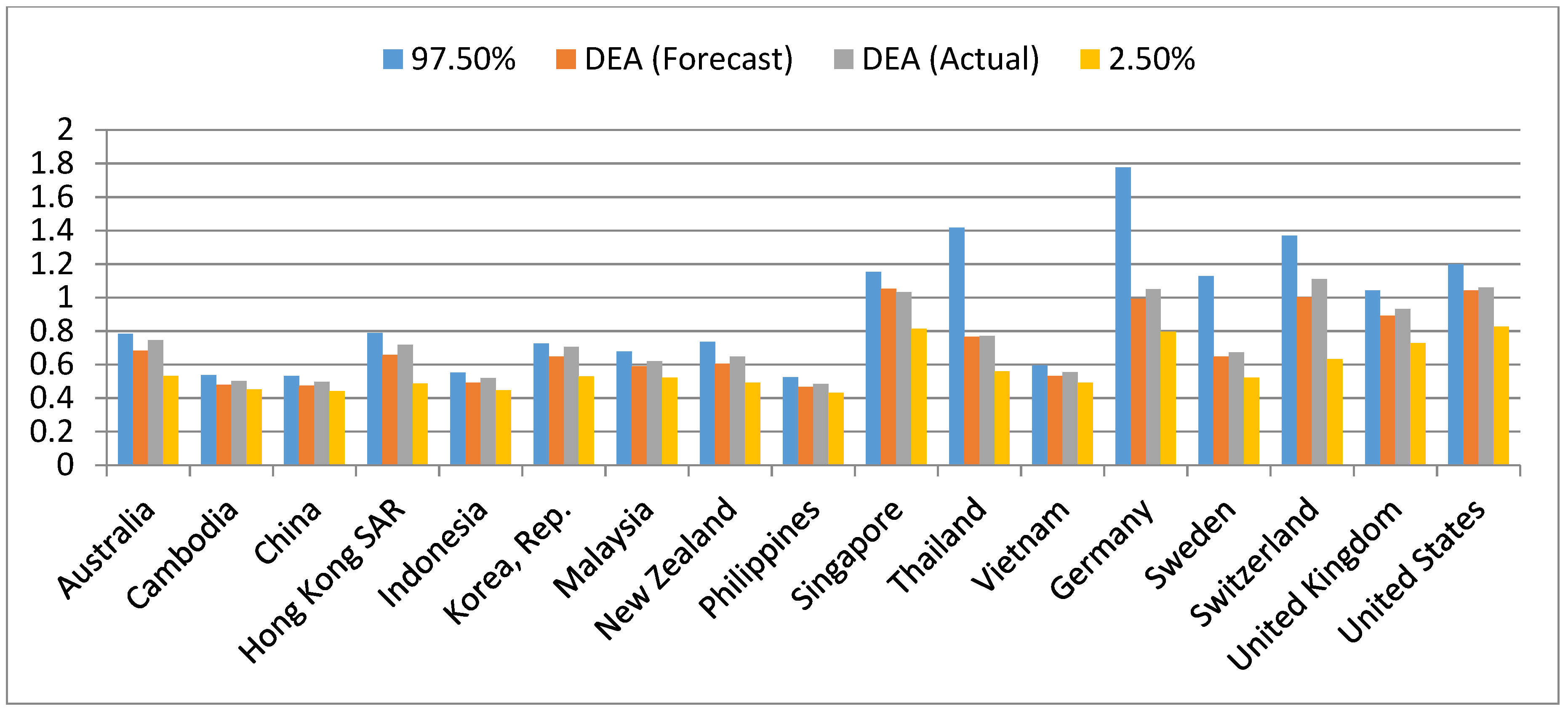
United States	1.199	1.042	2	1.060	2	0.827

provides the results of a basic indicator in 2017 for input/output of each DMU. At the same time, the authors added the actual super-SBM score for 2017 to compare real data and forecast data. The results shown in Figure 4 and Table 7 reveal little difference between the forecast efficiency levels and actual efficiency levels. Of the 17 countries, the actual 2017 scores of 17 are included in the 95% confidence interval. The average of forecast-actual over the 17 countries was −0.035 (−3.5%).

It was observed that the forecast of rank and score of 17 countries remained at a similar level to the actual. There was a slight change in ranking for Korea Rep., Germany, and Sweden. To be specific, Korea Rep. and Sweden were down one level; Germany increased one level compared to the actual. However, Singapore dropped abruptly four steps compared with the prediction from the top-ranked to the third, while Switzerland led the ranking from the third ranked.

3.4. Future Forecast Performance Evaluation Results

Figure 5 illustrates the overall picture of macroeconomics of 17 countries over time from the past to the future for each year in past (2013–2016), present (2013–2016), and future (2017–2020). During this time-series, the 17 countries (economies) as a whole experienced a slight change. The performance index estimates indicated that Singapore, Germany, Switzerland, and United States achieved sustainable performance. The average score of these economies remained at a high level, and is larger than 1. The 11 Asian developing area countries stood at just under 1. That is, they have not reached the effective threshold in macroeconomic management.

By using forecast data for 2017 and the following years, this research obtained the forecasting result of all DMUs for the subsequent years of 2018 to 2020 (detailed data are shown in Appendix A, Appendix B and Appendix C). Appendix A forecasts the indicators from 2017 to 2020; Appendix B forecasts a confidence interval from 2017 to 2020 of the Lucas weight of the past-present-furute model; and Appendix C assesses the macroeconomic performance over the time chain.

4. Discussions

The paper was inspired by “The Global Competitiveness Report” of the World Economic Forum [1] evaluating the global competitiveness of the countries/economies. In the whole study, the authors used the terms “economy” and “country” in a flexible way because of the political implications of some countries, in which the macroeconomic environment plays an important role in maintaining the sustainability of each economy. From the overall picture of global competitiveness, we focus on selecting countries that are emerging economies such as Singapore, China, Hong Kong SAR, Korea Rep, Thailand, Australia, Indonesia, New Zealand… (mainly in the Asia Pacific region) to be the main research objects. Besides, we selected the remaining five economies (including Germany, Sweden, Switzerland, United Kingdom, and United States) as advanced economies in the world. From there, the paper was compared and analyzed to see the overall picture of global macroeconomic performance.

By clearly defining the subject and referring to the methods of measuring macroeconomic effectiveness, the authors realize that DEA is an effective method to measure the performance of multiple decision-making units when putting research subjects (the economies) in the correlation. The advantage of the DEA method is that it combines many input/output indicators to assess the effectiveness of economies. This is confirmed in several past papers [11,12,13]. Besides, various contributions in the past using econometric approaches such as the Okun index, the Calmfors–Driffill index, or the OECD’s “magic diamond” considered all of the four main macro indicators, i.e., GDP growth, trade balance, inflation, and unemployment. Once again, the authors have a solid basis for selecting the input/outputs as presented in the study.

Our study is correlated with previous studies via the use of the DEA method to measure macroeconomic performance. Despite similarities with those of the research model, the results are significantly different due to the selection of inputs, outputs, and country of study. For example, Lovell [11] established a scalar-valued measure of an economy’s macroeconomic performance. The procedure was applied to a set of 10 Asian economies over a 19-year period from 1970 to 1988, with special attention paid to Taiwan. The four variables selected were GDP growth, employment, trade balance, and price stability. The results, i.e., the performance of the 10 economies, had been evaluated during part or the entire period from 1970 to 1988. However, the first point concerns the structure of the model, which contains no inputs and four outputs. It did not adequately reflect the real targets of macroeconomic policy. Moreover, although the data collected in the past are relative, the study was conducted on a small scale: 10 economies in Asia. Our study has produced outstanding results when selecting four indicators (government gross debt, real GDP growth, inflation rate, and unemployment rate) as input/output, in which a government gross debt indicator replaces Lovell’s trade balance indicator [11], and four indicators are set for the inputs and outputs of study. Data were collected from 17 economies, which show the main macroeconomic picture. Further, Cherchye [13] used a DEA model to evaluate a sample of 20 OECD countries covering the period from 1992 to 1996. The study provided a comparison of several synthetic indicators that merge the four separate indicators into a single statistic. The difference in this study and the current study is that countries are selected as DMUs and time to conduct research. Therefore, it is difficult to make comparisons from the results of the analysis. The highlight of the current study is predicting macroeconomic performance in the near future based on historical data.

The results from the research data show that research results are as close to the World Economic Forum’s ranking in the annual report. Specifically, advanced economies such as Switzerland, Singapore, and the United States always rank highly in macroeconomic performance. This also reflects the macroeconomic management success of the country. On the contrary, some economies in emerging markets such as those in Cambodia and the Philippines show less effective macroeconomic management capacity. In addition, the near future forecast data for the next four years gives the same results. On the other hand, the results from data analysis also show significant differences between the macroeconomic performance of emerging markets compared with those in the five advanced countries. This has been clearly demonstrated in the analysis of research results.

5. Conclusions

This paper provides an evaluation of the performance of institutions responsible for the conduct of macroeconomic and environmental policies in some economies. Similar analyses have been conducted previously, although they have been summarized into an evaluation of macroeconomic policies. This study appears to be the first of its kind to focus on performance evaluation by combining prediction models to provide overall circumstances and efficient tendencies for the 17 countries. The resampling model is based on these variations for gauging the confidence intervals of DEA scores, in which the first model was utilized by past-present data for estimating data variations imposing chronological order weights, which are supplied by Lucas series. The second model deals with future prospects. The analytical tools we have employed in this study are intended to improve upon previous treatments. DEA originated by Charnes and Cooper [5] is a nonparametric mathematical programming methodology that deals directly with input/output data. Using the data, DEA can evaluate the relative efficiency of DMUs and propose a plan to improve the inputs/outputs of inefficient DMUs. This function is difficult to achieve with similar models in statistics, i.e., stochastic frontier analysis. DEA scores are not absolute but relative, i.e., they depend on the choice of inputs, outputs, and DMUs as well as on the choice of model for assessing DMUs. DEA scores are subject to change; thus, data variations in DEA shoud be taken into account.

Application of the resampling model to a set of 17 economies over the period from 2013 to 2016 and forecasting for the period 2017 to 2020 generated the following conclusions: (i) the overall picture of macroeconomic performance of 17 countries was built based on DEA-integrated models for the period from 2013 to 2016; (ii) there appear to be significant differences between the quality of macroeconomic management in the 12 Asian developing countries and in the remaining five developed countries. This has helped consolidate the World Economic Forum’s annual rankings in the global competitiveness report [1]; (iii) when the four primary macroeconomic objectives are included in the performance evaluation analysis, we find that Switzerland, Singapore, and the United States have enjoyed the most successful macroeconomic management, while Cambodia, China, and the Philippines have suffered the least sucessful macroeconomic management; these conclusions are supported by the data. This is particularly relevant for developed countries, which historically have pursued macroeconomic policies designed to achieve an equitable income distribution.

Although this paper shows that a resampling model is a flexible and easy model of use to predict, this paper only focuses on a quantitative model, and the results reveal the relative performance. The authors will do more research of external environmental factors in the future. The comparisions with other quantitative and qualitative approaches will be a good research direction as well.

The main contribution of this paper is to provide an evaluation and forecast of macroeconomic policies of 17 countries. The research results may help to improve macroeconomic efficiency, to achieve economic growth, to reduce the ratio of inflation and unemployment, and toward a sustainable economic development. The findings in this study will provide policy-makers with incentives to improve macroeconomic indicators. The estimation results may give useful information and practical suggestions for governments to realize their collective goal of enhancing global competitiveness.

References

- The Global Competitiveness Report 2017–2018. Available online: http://reports.weforum.org/global-competitiveness-index-2017-2018/ (accessed on 26 April 2018).
- Koomans, T.C. An analysis of production as an efficient combination of activities. In Activity Analysis of Production and Allocation, Cowles Commission for Research in Economics; Koopmans, T.C., Ed.; Monograph No. 13; Wiley: New York, NY, USA, 1951. [Google Scholar]
- McCracken, P.; Carli, G.; Giersch, H. Towards Full Employment and Price Stability: A Report to the OECD by a Group of Idependent Experts; Organization for Economic Cooperation and Development: Paris, France, 1977. [Google Scholar]
- Calmfors, L.; Driffill, J. Bargaining structure, corporatism and macroeconomic performance. Econ. Policy 1988, 6, 13–61. [Google Scholar] [CrossRef]
- Charnes, A.; Cooper, W.W.; Rhodes, E. Measuring the efficiency of decision making units. Eur. J. Oper. Res. 1978, 2, 429–444. [Google Scholar] [CrossRef]
- Wang, C.N.; Li, K.Z.; Ho, C.T.; Yang, K.L.; Wang, C.H. A model for candidate selection of strategic alliances: Case on industry of department store. In Proceedings of the Second International Conference on Innovative Computing, Information and Control, Kumamoto, Japan, 5–7 September 2007; IEEE: Piscataway, NJ, USA, 2007. [Google Scholar]
- Yuan, L.N.; Tian, L.N. A new DEA model on science and technology resources of industrial enterprises. Int. Conf. Mach. Learn. Cybern. 2012, 3, 986–990. [Google Scholar]
- Wu, F.; Fan, L.W.; Zhou, P.; Zhou, D.Q. Industrial energy efficiency with CO2 emissions in China: A nonparametric analysis. Energy Policy 2012, 49, 164–172. [Google Scholar] [CrossRef]
- Egilmez, G.; Kucukvar, M.; Tatari, O. Sustainability assessment of US manufacturing sectors: An economic input output-based frontier approach. J. Clean. Prod. 2013, 53, 91–102. [Google Scholar] [CrossRef]
- Chang, M.C. Room for improvement in low carbon economies of G7 and BRICS countries based on the analysis of energy efficiency and environmental Kuznets curves. J. Clean. Prod. 2015, 99, 140–151. [Google Scholar] [CrossRef]
- Lovell, C.A.K. Measuring the macroeconomic performance of the Taiwanese economy. Int. J. Prod. Econ. 1995, 39, 165–178. [Google Scholar] [CrossRef]
- Lovell, C.A.K.; Pastor, J.T.; Turner, J.A. Measuring macroeconomic performance in the OECD: A comparison of European and non-European countries. Eur. J. Oper. Res. 1995, 87, 507–518. [Google Scholar] [CrossRef]
- Cherchye, L. Using data envelopment analysis to assess macroeconomic policy performance. Appl. Econ. 2001, 33, 407–416. [Google Scholar] [CrossRef]
- Tone, K.; Ouenniche, J. DEA score’ confidence intervals with past-preesent and past-present-future based resampling. Am. J. Oper. Res. 2016, 6, 121–135. [Google Scholar] [CrossRef]
- World Bank. Available online: https://data.worldbank.org/ (accessed on 15 November 2017).
- International Monetary Fund. Available online: http://www.imf.org/external/index.htm (accessed on 13 November 2017).[Green Version]
- Cook, W.D.; Tone, K.; Zhu, J. Data envelopment analysis: Prior to choosing a model. Omega 2014, 44, 1–4. [Google Scholar] [CrossRef]
- Wikipedia. Available online: https://en.wikipedia.org/wiki/Inflation (accessed on 13 November 2017).
- The Organization for Economic Co-Operation and Development (OECD). Available online: http://www.oecd.org/ (accessed on 24 November 2017).
- Tone, K. A slack-based measure of super-efficiency in data envelopment analysis. Eur. J. Oper. Res. 2002, 143, 32–41. [Google Scholar] [CrossRef]
- Tone, K. A slack-based measure of efficiency in data envelopment analysis. Eur. J. Oper. Res. 2001, 130, 498–509. [Google Scholar] [CrossRef]
- Efron, B. Bootstrap Methods: Another Look at the Jackknife. Ann. Stat. 1979, 7, 1–26. [Google Scholar] [CrossRef]
- Fisher, R.A. Frequency distribution of the values of the correlation coefficient in samples from an indefinitely large population. Biometrika 1915, 10, 507–521. [Google Scholar] [CrossRef]
- Fisher, R.A. On the interpretation of ÷2 from contingency tables, and the calculation of P. J. R. Stat. Soc. 1922, 85, 87–94. [Google Scholar] [CrossRef]
Figure 1.
Research process.
Figure 2.
Panel data results.
Figure 3.
DEA score and confidence interval with 500 replicas.
Figure 4.
Confidence interval, forecast score, and actual 2017 score: forecast by Lucas model.
Figure 5.
The macroeconomic performance over time (2013–2020).