Towards Efficient Resource Utilization Exploiting Collaboration between HPF and 5G Enabled Energy Management Controllers in Smart Homes

Abstract

The influence of Information Communication and Technology (ICT) in power systems necessitates Smart Grid (SG) with monitoring and real-time control of electricity consumption. In SG, huge requests are generated from the smart homes in residential sector. Thus, researchers have proposed cloud based centralized and fog based semi-centralized computing systems for such requests. The cloud, unlike the fog system, has virtually infinite computing resources; however, in the cloud, system delay is the challenge for real-time applications. The prominent features of fog are; awareness of location, low latency, wired and wireless connectivity. In this paper, the impact of longer delay of cloud in SG applications is addressed. We proposed a cloud-fog based system for efficient processing of requests coming from the smart homes, their quick response and ultimately reduced cost. Each smart home is provided with a 5G based Home Energy Management Controller (HEMC). Then, the 5G-HEMC communicates with the High Performance Fog (HPF). The HPFs are capable of processing energy consumers’ huge requests. Virtual Machines (VMs) are installed on physical systems (HPFs) to entertain the requests using First Come First Service (FCFS) and Ant Colony Optimization (ACO) algorithms along with Optimized Response Time Policy (ORTP) for the selection of potential HPF for efficient processing of the requests with maximum resource utilization. It is analysed that size and number of virtual resources affect the performance of the computing system. In the proposed system model, micro grids are introduced in the vicinity of energy consumers for uninterrupted and cost optimized power supply. The impact of the number of VMs on the performance of HPFs is analysed with extensive simulations with three scenarios.

1. Introduction

Increasing demand for electricity and environmental pollution create an alarming situation for governments and electricity producing companies. The companies are encouraged to utilize renewable energy sources to overcome carbon emission. Unfortunately, more than 65% of electricity is wasted during the production, transmission and distribution [1]. Efficient power system consists of control, information and communication technologies called Smart Grid (SG). Energy in SG is managed on the supply side for production, transmission and distribution. On the demand side, consumers are educated to optimize their energy demand to reduce cost.

SG is the combination of Information Communication and Technology (ICT) and the conventional power grid. SG monitors and controls the power flow for efficient and reliable electricity provision than the traditional power grid. The heterogeneous architecture of SG welcomes new technologies to tackle a variety of technical challenges. To manage millions of energy consumers with billions of requests, utilities extend ICT systems with the cloud. A cloud based environment is equipped with high storage, maximum resources with efficient resource utilization and high performance [2,3]. However, a huge amount of traffic of requests on the network for cloud based centralized computing system creates a bottleneck for bandwidth. In SG, an extensively huge number of requests with low bandwidth challenges real-time based SG applications.

In SG, on the demand side, energy in SHs is efficiently managed on the bases of information of appliances load demand and tariff rates from the supply side. Delayed information sharing between supply and demand sides keeps the inefficient operation of appliances. Cloud based SG suffers from latency and security issues; to overcome this, fog is introduced. The fog extends the cloud services on the edge of the network. In SG, fog is placed between utility and end users to provide computing services for energy requests. End users or energy consumers receive responses of computed requests from fog in near-real-time. In this paper, High Performance Fog (HPF) is introduced for each group of buildings with multiple SHs to process their requests of energy, generated every hour. The processed requests are responded back in near-real-time.

In computing systems, resource sharing techniques are used for efficient resource utilization. In cloud and fog computing environments, virtual resources are created on the physical resources for high performance and efficient resource utilization. Multiple virtual resources are created and scheduled to entertain the huge heterogeneous data.

In this paper, the cloud-fog based system model is proposed to tackle delayed responses and permanent storage of consumers’ data for energy demands. In the system model, the requests of energy are received on HPF to get processed and responded back in near-real-time instead of processing on the cloud. Six regions with groups of residential buildings connected with HPFs are considered. HPFs are connected with Micro Grids (MGs), residential buildings and the cloud. MGs are placed closer to the buildings. The utility is connected with the cloud. A huge number of requests from groups of residential buildings are generated and receive on HPFs to get processed. Provision of energy to the buildings either from SG or utility is decided on the fog. HPFs reduce the computing burden of the cloud as well as tackle the latency and data security issues [4].

In computing systems, resource sharing techniques are used for efficient resource utilization. In cloud and fog computing environments, the virtual resources are created on the physical resources for high performance and efficient resource utilization. Multiple virtual resources are created and scheduled to entertain the huge heterogeneous data. In this paper, the cloud-fog based system model is proposed to tackle delayed responses and permanent storage of consumers’ data for energy demands. In the system model, the requests of energy are received on HPF to get processed and responded back in near-real-time instead of processing on the cloud. Six regions with groups of residential buildings connected with HPFs are considered. HPFs are connected with Micro Grids (MGs), residential buildings and the cloud. MGs are placed closer to the buildings. The utility is connected with the cloud. A huge number of requests from groups of residential buildings are generated and received on HPFs to get processed. Provision of energy to the buildings either from SG or utility is decided on the fog. HPFs reduce the computing burden of the cloud as well as tackle the latency and data security issues [4].

The selection of potential data center, installed with Virtual Machines (VMs), is made by service broker policies. The service broker policies route the requests to the potential data center for efficient processing and response. These policies use different constraints like the location of the data centers from the user base and performance of the data centers. VMs are allocated with a number of requests to process; however, efficient allocation with a balanced load on each VM is maintained with variety of algorithms. In this paper, Optimized Response Time Policy (ORTP) selects the data center or the fog to route the requests on it. The algorithms, First Come First Serve (FCFS) and Ant Colony Optimization (ACO) allocate VMs to the requests. The simulations of three scenarios validate the appropriate number of VMs in comparison to the capacity of physical system enhance the performance of Response Time (RT), Processing Time (PT) and the cost.

1.1. Motivation

In [5], a cloud based model is proposed to facilitate the consumers within a limited geographic area. A hybrid of a genetic algorithm and particle swarm optimization algorithm is proposed to balance the load of requests on VMs. The experimental outcomes of hybrid algorithms validate the efficient processing cost as compared to state-of-the-art algorithms. However, the authors in [6] resolved the issue of resource allocation by implementing the ant colony system, named “MORA-ACS“. The performance is evaluated based on PT, energy consumption and standard deviation with round robin service broker policy. A cost oriented model for demand side management by optimum allocation of the cloud resources is proposed in [7]. This model gives the consumers a flexibility in resource optimization and cost minimization.

The state-of-the-art system models are inefficient to cater the huge amount of heterogeneous data. The cloud and fog resources consume high energy for processing of huge requests and compromise the performance. A paradigm is needed for an optimized performance on both cloud and fog based SG systems. The proposed system model reduces the RT, PT and the cost. In this paper, a system model with service broker policy and load balancing algorithm is proposed to tackle the latency and resource allocation problem.

1.2. Problem Statement

In SG, energy crises have been a serious concern for many years. The researchers are addressing such issues by proposing energy management techniques using load shifting and dynamic pricing [8]. The authors in [9] extend energy management with efficiency and reliability of HEMS in [8]. Towards improvement on [9], in [10], the authors proposed an infrastructure to allocate cloud resources with flexibility and cost efficiency for demand side management in smart homes. However, delayed responses from the cloud are not suitable for the delay sensitive applications. Thus, authors in [11,12,13] support fog computing over cloud because of increasing demands. VMs are installed on computing environments for efficient resource utilization and processing. In [14], experimental analysis is conducted to evaluate the number of VMs for a physical machine in energy efficient way. However, the authors concluded that the capacity of VMs and their collocation reduce the job completion time. To check the effects of the number of dynamic VMs placement on physical machines for time and cost sensitive applications of SG is the challenging task that is not addressed in the papers mentioned above.

1.3. Contributions

The contributions of this work are summarized as follows:

• For monitoring energy management, residential buildings are classified into six regions based upon continents of the world using the “CloudAnalyst” simulator [15].
• Integration of HPF between the cloud and residential buildings reduces the cost and latency.
• HPF processes the requests and responses back instead of sending the requests to the cloud which suffers from latency and data security issues.
• Energy consumption and user demands are monitored in near real-time.
• RT, PT and computational cost are reduced by optimizing the VMs with a load of requests on the HPFs.
• The management and processing of the requests are optimized on the VMs using FCFS and ACO algorithms.
• We have dynamically selected of the number of VMs on the HPFs for efficient performance and the reduced cost of the system.

1.4. Paper Organization

The remainder of the paper is organized as follows: related work is described in Section 2. The proposed framework is presented in Section 3. Service broker policy and VM load balancing algorithms are presented in Section 4. Results and discussion are explained in Section 5. In Section 6, the conclusions are provided.

2. Related Work

Cloud and fog computing provide a virtual environment to provide efficient resource sharing to the connected consumers. These resources are allocated to increase the use of VMs instead of using physical machines, for energy consumption reduction. However, fog computing extends the concept of cloud computing by reducing the load on cloud. To maintain the load of requests of connected consumers on cloud and fog, different load balancing algorithms are applied. These algorithms are used to schedule the requests and allocate the number of requests to VMs. Mostly, both heuristic and static algorithms are used for load balancing among VMs as in [16,17,18,19,20].

The author in [21] proposed a cloud load balancing algorithm for load balancing on cloud and compare the results with previously used algorithms applied for the same scenario. The performance of the proposed algorithm is better than the other algorithms. Therefore, load is balanced when a multiple number of users logged in at the same time. The authors present a new communication model using two models: the cloud based demand response model and distributed demand response model for computing the communication efficiency with reference to optimal resource allocation [22]. This scheme procures the high cost by incorporating the high demand response scenarios. The authors presented a cost oriented model for demand side management by optimally allocating the cloud resources [7]. This model gives consumers the flexibility in resource optimization which results in cost minimization.

The authors proposed a new load balancing algorithm in [23]. For efficient task allocation, the load is balanced using a proposed algorithm. The mathematical model is used to allocate low power tasks and others are allocated to human resources. However, the proposed algorithm improves the throughput by reducing the tardiness. However, the authors in [24] compared multiple service broker policies to estimate the PT. However, the round robin scheduling algorithm is used to compare broker policies. Three service broker policies are compared for RT and request PT. These policies include service proximity, optimise RT and dynamically reconfigure with load service broker policies. In [25], a Service Oriented Middleware (SOM) model is proposed for the integration and utilization of fog and cloud of things (CoTs). The smart city ware summarized the components and services used for applications accessed through the service oriented model in a smart city.

In [26], the author proposed an architecture which is decentralized cloud based architecture. The authors aimed to schedule the requests coming from consumer side in a real-time environment. For this purpose, they have done simulations for real-time electric load data of Toronto city in Canada. However, a pricing model is proposed for energy load optimization during the on peak hours by maintaining stability of MG. A new service broker policy is proposed for data center selection in [27]. The authors conduct master fuzzy context for provisional fuzzy logic and fuzzy rules are designed for SG RT and data center priority.

The authors monitor the bulk power grids with grid cloud concept [28]. This concept is an open source platform for real-time data estimation. In grid cloud, SG is supported on Amazon web services and is similar to the cloud platform. The authors used cloud tools for cost reduction, software oriented redundancy to overcome the failures and different methods to secure the sensitive data. The authors proposed a Privacy Preserving Fog-enabled Aggregation (PPFA) architecture in [29]. The fog node collect data from smart meters and estimate the cost on fog level aggregation; however, cloud or the utility supplier calculates the total cost while aggregating all fogs. In [30], authors have conducted an analysis that shows that cloud based utilities improve the SG ecosystem and how services on fog computing work for the same scenario. The algorithms on fog work while interplaying with cloud computing and check that is it applicable on a real-time environment by providing delay free services to SG.

The author in [31] proposed a certificate-less provable data possession method. The method is proposed for cloud based SG applications. The main focus of the paper is to provide sufficient storage, processing capacity and security using data management system proposed to support SG applications. In addition, the authors in [32] used Wavelet Recurrent Neural Network (WRNN) predictors. The solutions are given for a cloud distributed model and balance for energy management is also achieved for available devices by means of prediction. The power is used according to the requests coming from consumer side due to predictions made using WRNN predictors.

The cloud facilitates the consumers with: computing, storage and highly centralized connectivity. However, it suffers from latency, security and downtime issues. For improving the latency, flexibility, resiliency and reliability of the cloud computing services, a new scheme is proposed in [33] and implemented using devices profile for web services, which presents energy management as a service using fog computing environment. Two energy management prototypes are developed in this methodology: home energy management prototype and MG energy management prototype for cost minimization and latency reduction.

Similarly, a Transmission Control Protocol/Internet Protocol (TCP/IP) based single hop network is proposed in fog data centers with adoptive resource scheduler for energy efficiency in [34]. The requests of traffic arrive at fog data center where scheduler configures the VMs for minimum energy dispatching. Moreover, requests are instantaneously processed and responded to vehicular clients. In [35], a platform of fog-of-everything with Internet-of-everything is proposed for the required satisfactory quality-of-service. The proposed algorithm in the platform saves more energy as compared to existing state-of-the-art algorithms for the fog data centers. Fog and Internet-of-everything are also integrated in [36] and formed fog-of-everything like [35]. However, the authors of [36] performed simulations to study the reduced energy and enhanced the performance of fog computing for huge data.

The literature discussed above is summarized in

Table 1. Related work.

Technique (s)	Features (s)	Limitation (s)
Proposed hybrid of AMLB and Throttled [16]	Improved RT, PT, throughput and reduced operational cost	Static data implementation
Proposed, Autonomous Agent Based Load Balancing algorithm [17]	Increase throughput, resource utilization, reliability and scalable	Dynamic iterative technique has high time and space complexity
Proposed, PSO based load balancing algorithm [18]	Reduce task overhead and enhance resource utilization	Redundant and costly, evaluation of a VM has to wait until first completes
Proposed, linear programming based Dynamic Weighted Live Migration (DWLM) mechanism [19]	Runs information based policy, improved migration time, throughput and RT	Dynamic evaluation has high time and space complexity while LP waits until dynamic migration evaluation is performed. Costly and complex
Proposed, load and processing efficient architecture with two load balancing algorithms [21]	The load balancing architecture validates virtual and physical servers’ performance	The high number of connections compromise the performance
Proposed colorful ants based load balancing algorithm [23]	Dynamic load balancing, HR ranking based tasks queue	The time complexity of the algorithm is high due to iterative nature and not appropriate for huge requests
3 service broker policies and 3 load balance algorithms [24]	RT and PT using closest Data Center policy is optimized as compared to rest	Static requests data limit the understanding of performance with Closest Data Center policy
Proposed, Service oriented architecture and design of middleware for cloud and fog computing in smart city [25]	Mobility, heterogeneity, real-time response and dta security	Limitation of fog resource, limit of number of devices registration, Java has limitation for implementation
Proposed, an open source GridCloud platform for bulk interconnected power grid [28]	Data security, reduced cost and software based failure overcome	Geographic diversity compromise performance of the cloud, Latency
Proposed, Cloud and Fog level aggregation for SG [29]	data security, robust, Direct link of smart meters with fog node	Security key sharing for huge number of users is expensive, limitation of downstream bandwidth
Proposed the fog based model for SG [30]	Mix of fog and cloud computing assures high computation with security and mobility	Redesign and development of delay sensitive applications for fog node with migration characteristics, New SG service services need to develop, Security challenges between cloud and fog nodes
Proposed, Management architecture predictive system for power generation from integration system and power consumption using cloud distribution for energy dispatch [32]	Real-time processing, Prediction of power generation and load demand	Number of nodes between power generation and cloud node and between cloud node to power consumers cause latency issues
Proposed, fog computing as energy management platform [33]	Open source hardware and software for customized services, scalability, adaptability, interoperability, scalability and connectivity of devices with fog, energy management	System deployment of residential sector is challenging due to low budget, operational and maintenance cost are additive cost and important for residents

. From the literature, it is analysed that fog computing helps to maintain and reduce the load of cloud efficiently. Multiple algorithms are introduced for load balancing and new service broker policies are proposed in different paper. However, using VMs, the results are improved and cost is reduced as compared to using physical machines.

3. System Model

In the proposed system model Figure 1, six geographic regions with groups of buildings are considered for simulation. Each building has multiple Smart Homes (SHs) or apartments with Internet of Things (IoT) based appliances. Every home has a smart meter with 5G enabled controller to monitor, control the IoT based appliances and communicate with the controller of the building. Each building communicates using the controller with fog node in the region for processing of energy requests of SHs. Fog is connected with MG and the cloud. If demands of SHs are not met by MG, then fog requests the utility via the cloud to fulfill the demand. Fog transmits the data of consumers to cloud for permanent storage and future usage. The communication takes place between home appliances and smart meter, building controller and smart meters, fog and the controllers, MG and fog, utility and fogs, and cloud and fogs; however, power flows from utility and MG to the buildings. It is assumed that every communicating device has an IoT module to share data over the Internet. Parameters for the group of buildings considered for the proposed system model are given in

Table 2. Parameters for groups of buildings.

Group of Buildings	Region	Number of Buildings	Requests/Building/hour	Data Size/Request (bytes)	Number of MGs Available
G1	R1	100	100	128	3
G2	R2	90	70	128	4
G3	R3	72	66	128	5
G4	R4	59	59	128	2
G5	R5	86	80	128	4
G6	R6	70	60	128	2

.

Fog receives requests from the building controller for energy demands. Fog prefers MG, due to cheaper energy as compared to utility and instructs to facilitate the required SH in the building. If MG has insufficient power, then it responds to the fog accordingly. The fog requests the utility via the cloud to meet the energy demand of the building. SHs generate frequent energy requests and send to respective fog node in the region for energy demands. When hundreds of SHs generate hundreds of thousands of requests for a day then computational performance becomes challenging. HPFs are introduced between cloud and buildings (end users). HPF, unlike cloud, has low latency, lesser PT and RT with data security. The communicating modules in the system model are monitored and controlled using IoT based applications over web services.

Fog is like a small cloud; however, it has limited resources as compared to the cloud. It is placed close to the end devices (end users) and extends the cloud services on the network edge with high performance and real-time responses. The resource sharing techniques are used for efficient resource utilization in cloud and fog computing. VMs are installed on the fog for resource sharing to efficiently process the huge number of energy requests. Load of requests on VMs affect the performance, hence load optimizing algorithms are used. In this paper, FCFS and ACO algorithms are implemented for load balancing over VMs. However, selection of potential data center on fog node is made by service broker policies; ORTP. The simulations are performed with the simulator “CloudAnalyst” [15], in which calibration of fog parameters are tuned, as shown in

Table 3. Input parameters regarding HPF.

	Parameter	Value
VM	Image Size	10,000 MB
	Memory	512 & 1024 MB
	Bandwidth	1000 Mbps
HPF	Architecture	X86
	Operating System	Linux
	VM manager	Xen
	Number of Machines	20
Machines	Memory	2048 MB
	Storage	100 GB
	Available BW	10,000
	Number of processors	4
	Processor speed	100 MIPS
	VM Policy	Time Shared
	Homes Grouping Factor	1000
	Requests Grouping Factor	100
	Executable Instruction Length	100

.

VMs are the programs that mimic the operations of physical machines. Resources of physical computing machines are divided logically to create VMs. Hence, physical resources are shared using VMs to enhance the performance and unbound the specifications of resources. However, too many VMs on physical resources limit the capacity of the resources; hence, it is assumed that overall performance of the system should not be compromised. In this paper, the system model is proposed for SG applications, in which a huge number of requests are generated in a day for every hour from residential buildings and are sent to the HPFs. The load of requests is routed on data servers for RT optimization as well as on VMs which are allocated with balanced load of requests to reduce the PT. Three scenarios are implemented with the same specification of hardware; however, VMs are doubled in $scenario2$ as compared to $scenario1$ and doubled in $scenario3$ as compared to $scenario2$.

MGs are equipped with Renewable Energy Sources (RES) which are placed closer to consumers to save power losses. In this paper, five MGs, as shown in Equation (1), are taken with a battery storage system, RESs: photovoltaic arrays and wind turbines. MGs are preferred to use when the utility has on-peak hours, while, during off-peak hours, RESs store the energy. The set of regions (R) with a set of buildings (GB) are given in Equations (2) and (3):

$$MG=M{G}_1,M{G}_2,\dots ,M{G}_n,wheren=5,$$

(1)

$$R=R_1,R_2,\dots ,R_i,wherei=6,$$

(2)

$$GB=G{B}_1,G{B}_2,\dots ,G{B}_j,wherej=6.$$

(3)

In the proposed scenario, each region has one group of buildings with SHs or apartments. On average, 1000 are off-peak users and 100 are on-peak users. Cost of energy consumption is reduced in off-peak hours—this is why most users are off-peak consumers. Each region has an HPF computing node with memory, storage, number of processors, operating system and VM manager, etc. HPFs store data temporary and transfer to the cloud for permanent storage. Parameters of HPFs are given in Table 3. A huge number of requests are processed on HPFs; however, an efficient load of requests over VMs and selection of potential data centers reduces PT and RT for the consumers’ requests. Moreover, the groups of buildings generate peak load of requests in a day. The peak hours of “G1”, “G2”, “G3”, “G4”, “G5” and “G6” are during 4:00 p.m. to 11:00 p.m., 8:00 a.m. to 5:00 p.m., 7:00 p.m. to 11:00 p.m., 6:00 p.m. to 10:00 p.m., 3:00 a.m. to 11:00 a.m. and 3:00 a.m. to 11:00 a.m., respectively. Peak load of requests also affects the performance and overall computation cost which ultimately electricity users have to pay. Tuning the parameters of Table 2 along with the peak load of request time in a day in the CloudAnalyst is implemented with three scenarios.

4. Problem Formulation

A huge number of energy requests x arrive at HPF to get processed with minimum processing and RT. The set of all x requests is $RQ=\{R{q}_1,R{q}_2,\dots ,R{q}_x\}$ and the set of all v VMs installed on HPF is $VM=\{V_1,V_2,\dots ,V_v\}$. Minimization of PT is the goal and is shown in Equation (4):

Minimize

$$T_P^{avg}=\frac{{\sum }_{i=1}^v{T}_{Pr}\left(i\right)}{v}$$

(4)

subject to

$$T_{Pr}\left(i\right)=\frac{{\sum }_{a=1}^{x}R{q}_l\left(a\right)}{P{R}_{speed}\left(i\right)},\forall iϵ1,2,\dots ,v,$$

(5)

$$Rq\ge 1.$$

(6)

Average PT of all VMs is calculated as shown in Equation (7):

$$T_{AvgPr}^v=\frac{{\sum }_{i=1}^v{T}_{Pr}}{v}.$$

(7)

When a request is sent to the computational environment for processing, the sum of network delay, PT and the very first response to the consumer is called RT. It is also defined as the difference of arrival and finishing time of the task at fog addition to network or transmission delay time. The RT of a task j is calculated as Equation (8) where $FT\left(j\right)$ is finishing time of task j, $AT\left(j\right)$ is arrival time and $T_{delay}\left(j\right)$ is the transmission delay. Average RT of all x requests is calculated as in Equation (4):

$$RT\left(j\right)=FT\left(j\right)-AT\left(j\right)+T_{delay}\left(j\right),\forall jϵ1,2,\dots ,x,$$

(8)

$$R{T}_{avg}=\frac{{\sum }_{j=1}^{x}RT\left(j\right)}{x}.$$

(9)

Transfer of all data requests depends on the size of bandwidth $BW$. Transfer time of all data requests is calculated as in Equation (10),

$$T_{Transfer}=\frac{Dat{a}_{size}}{BW}.$$

(10)

4.1. Operational Cost

Operational cost is added in the user’s bill and computed as the cost of VMs, DT and MG. VMs have fixed or one time and recurring cost. Fixed cost is associated with the physical equipment and its installation. The recurring cost associated with the storage size, temporary memory, size and number of requests received or sent and bandwidth of VM. In this paper, the recurring cost is taken as VM cost and calculated as shown in Equation (11):

$$\begin{array}{c}VM\_Cost=Storage\_Cost\times VM\_size+RAM\_Cost\times \\ RA{M}_{VM}+BW\_Cost\times VM\_BW.\end{array}$$

(11)

Cost of MG also has fixed and recurring costs. Fixed cost depends on type and size of energy sources and their installation. The cost of energy produced depends on efficiency of production, maintenance and energy demand which is recurring cost of MG. Each MG has own recurring cost depending on size and demand; however, average cost of all MGs is calculated as in Equation (12):

$$M{G}_{AvgCost}=\frac{{\sum }_i^{m}M{G}_i}{m},$$

(12)

where m are number of MGs in a region. Cost of DT depends on total data size and cost per unit data. Total cost of data to be transferred is calculated as in Equation (13),

$$Dat{a}_{tCost}=Dat{a}_{size}\ast Cos{t}_{uData},$$

(13)

where $Dat{a}_{tCost}$ is the total cost of all data $Dat{a}_{size}$ times cost per data size $Cos{t}_{uData}$. Operation cost is the total cost of VM, MG, DT and calculated as in Equation (14). Total operational cost is the sum of costs of VM, MG and DT, as shown in Equation (14),

$$T_{OpCost}=VMCost+MGCost+Dat{a}_{tCost}.$$

(14)

4.2. Service Broker Policy

Service broker policy selects potential data center of efficient processing and RT. If multiple fog nodes, each with the single data center, are accessible for a user; then, service broker policy selects a potential fog node (fog data center) to route the traffic of requests on it. Selection is made on the bases of a variety of parameters—for example, PT, resource availability and RT, etc., by defining the policies to route the traffic of requests [37]. In this paper, ORTP is used to select potential data center in fog node.

Optimized Response Time Policy

This service broker policy makes selection of potential fog using the following points:

• Index of available HPFs in a region is maintained,
• Check the history in which HPF provides best RT in the history,
• The request coming from the clusters are assigned to the HPF located on the same region with best RT.

4.3. VM Load Balancing Algorithms

The load balancing algorithm helps to balance the load requests on multiple VMs for efficient processing. The efficiency of load balancing of algorithms varies and two of them are discussed in detail as below.

4.3.1. FCFS VM Load Balancing Algorithm

In the FCFS algorithm, the order in which requests arrive on the data center is allocated to VMs, accordingly. When huge requests arrive on data center, then these are put in wait in a pool in the same order as they are received. Each request is assigned with time or incremental priority tag. The algorithm picks the first request by calculating tag associated with it and prefers the earliest request to feed into the system for processing. The system has VMs which receive these requests for processing on FCFS bases. The algorithm has steps given in Algorithm 1.

Algorithm 1: FCFS

1: Input the requests along with their burst time $\left(b_t\right)$  2: Find waiting time $\left(w_t\right)$ for all requests.  3: The request comes first, need not to wait so, waiting time  4: Request 1 will be 0  5: wt[0] = 0  6: Find waiting time for all other requests i.e.; for Request = i +1 do  7: $w_t\left(i\right)=b_t(i-1)+w_t(i-1)$  8: Find turnaround time $\left(T_t\right)$ for all requests  9: $T_t\left(i\right)=w_t\left(i\right)+b_t\left(i\right)$ 10: Find average waiting time 11: $Total\_w_t\left(i\right)/No.ofProcesses$ 12: Similarly, find average turnaround time 13: $Total\_T_t\left(i\right)/No.ofProcesses$

4.3.2. ACO VM Load Balancing Algorithm

ACO algorithm is inspired from the behavior of ants when they search for food. Ants have no eyes and use pheromones chemical for their route to search the food. When plenty of food is found, then others are directed to the same destination from the nest with multiple paths using swarm intelligence. Initially, ants have multiple paths; however, after some time, the shortest path is chosen using swarm intelligence. Ants follow pheromones, which can be evaporated and the chance of availability from one location to other is also reduced. Hence, the performance of finding or calculating the shortest path is affected. Availability of pheromone is probabilistic; hence, ACO is a probabilistic meta-heuristic problem solving technique. The optimized solution inspiring from the behavior of ants is calculated with Equation (15):

$$p_{ij}^d=\frac{{\left({\tau }_{ij}\left(t\right)\right)}^{\alpha }\times {\left({\eta }_{ij}\left(t\right)\right)}^{\beta }}{\sum s\in J_{d\left(i\right)}{\left({\tau }_{is}\left(t\right)\right)}^{\alpha }\times {\left({\eta }_{is}\left(t\right)\right)}^{\beta }},$$

(15)

where $p_{ij}^d$ is the probability of pheromone, ${\tau }_{ij}\left(t\right)$ between i and j ants at time t. $\tau$ and ${\eta }_{ij}\left(t\right)$ are heuristic factors with coefficients of $\alpha$ and $\beta$. The ACO algorithm has steps given in Algorithm 2.

The time required to allocate available number of requests on the VMs is called time complexity of ACO. The time complexity from one pheromone’s position to other is $O\left(n\right)$ for n positions. For iteratively visiting all positions, the time complexity is $O\left(n^2\right)$. This exponential increase of time is too high for large instances. Hence, in this paper, the PT and RT for ACO are higher as compared to FCFS in $Scenario$ 1. The time complexity differences in $Scenario2$ and $Scenario3$ are higher as compared to $Scenario1$ due to a higher number of VMs. Local search is implemented in each fog computing for VM allocation; hence, space complexity is linear $\mathsf{\Omega }\left(n\right)$ while a global solution of ACO has space complexity of $\mathsf{\Omega }\left(n^2\right)$. The space and time complexity of ACO are very high.

In this paper, requests are the food and VMs are ants while HEMC acts as a nest of ants and generates requests and sends to HPF using 5G technology. The potential VM is selected by evaluating the availability and capacity for every request. Hence, before allocating the VM, the probability and suitability of VMs are updated in the list. Thus, iterative update and prioritization increase the time for manipulation.

The high time and space complexity of ACO make it unsuitable for huge data (e.g.; more than 3800 data requests [38]). For huge data, ACO traps in local optima. However, in this paper, number of requests or data are small and does not trap in local optima. However, time complexity is very high as compared to FCFS. It is assumed that probability of pheromone evaporation is reduced. Moreover, co-efficients $\alpha$ and $\beta$ are reduced to control local optima of ACO.

Algorithm 2: ACO

1: ACO parameters initialization: pheromone, routes, iteration  2: Solution = 0  3: Iteration = 1  4: Probability of allocation of VM computed using equation 15  5: Random allocation of tasks to VMs  6: The value of VM is inserted into list of VMs  7: Repeat the step until the completion of tour of ants  8: Compute the Solution  9: Calculate the distance between source to destination 10: Update the pheromone 11: Again calculate the distance 12: For every edge update the pheromone locally 13: Optimal solution is replaced by current solution 14: Continue the process until best optimal solution 15: Display the results

5. Simulation Results and Discussion

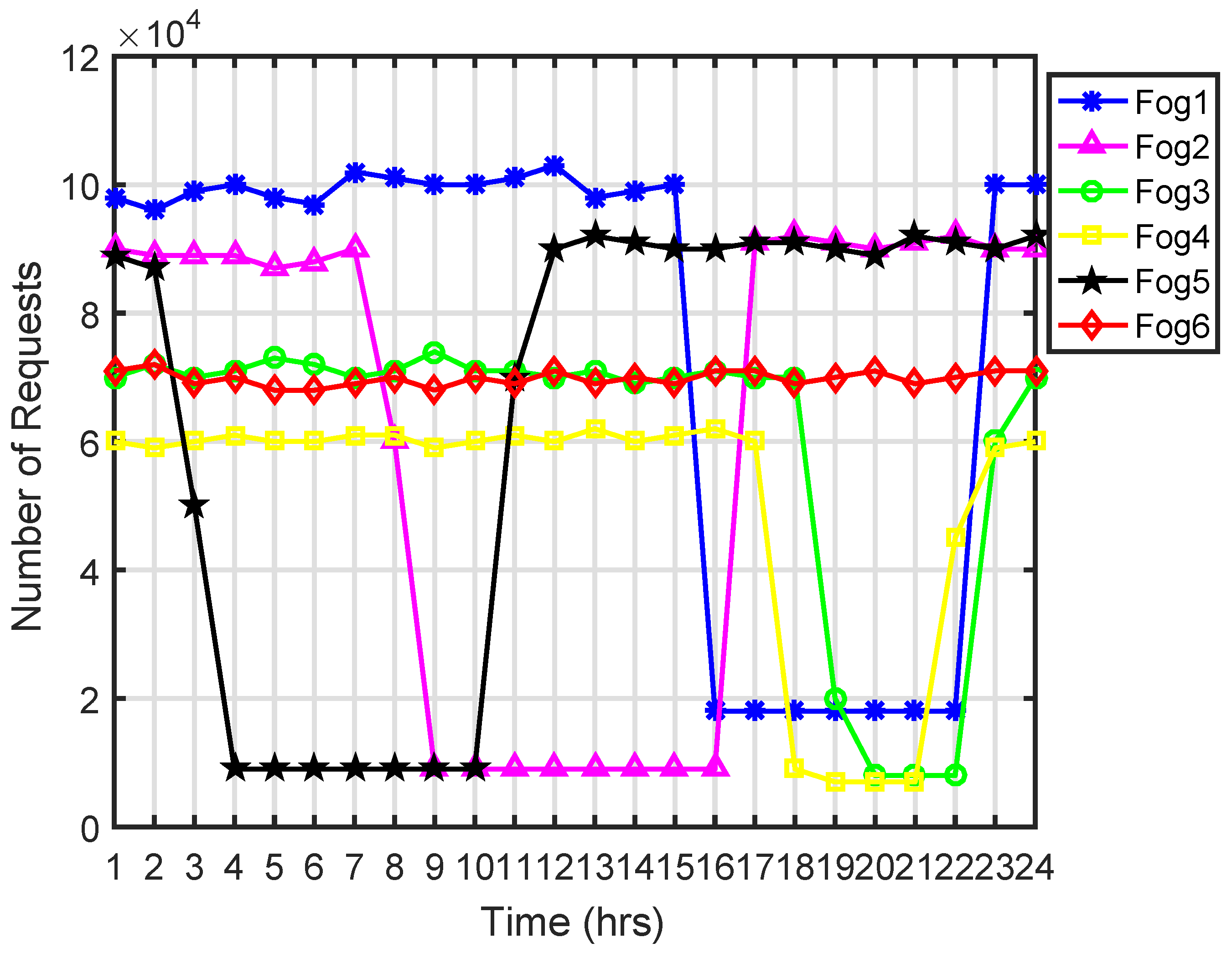
In this paper, ORTP selects the potential HPF or data center. Requests are assigned to VMs using FCFS and ACO algorithms. Three scenarios with 25, 50 and 100 VMs on the HPFs are considered. Every hour, a huge number of requests arrive at HPF, as shown in Figure 2, which are allocated to VMs using FCFS and ACO. Each scenario is also implemented with the cloud-based centralized system. In the system, we consider all groups of buildings are connected with the cloud which has an equivalent number of requests and resources, as the sum of all HPFs.

5.1. Scenario 1

In the scenario, there are 25 VMs on HPFs with a group of buildings generating requests and send to HPFs every hour, as shown in Figure 2. The requests are allocated on VMs using ACO and FCFS load balancing algorithms. The RT of the requests is measured in milliseconds for each group of buildings and their average, minimum and maximum RT is given in

Table 4. Response time of each group of buildings for ACO.

Group of Buildings	Average (ms)	Minimum (ms)	Maximum (ms)
G1	52.31	38.82	64.63
G2	51.29	39.99	66.39
G3	52.47	40.22	66.60
G4	52.31	38.67	64.17
G5	54.66	41.24	70.15
G6	54.92	42.28	71.27

using the ACO algorithm.

The PT of each HPF with the given scenario using ACO algorithm is given in

Table 5. Processing time of each HPF for ACO.

HPF	Average (ms)	Minimum (ms)	Maximum (ms)
HPF1	2.59	0.04	9.82
HPF2	1.58	0.03	6.18
HPF3	2.64	0.03	9.06
HPF4	2.63	0.04	9.93
HPF5	4.79	0.08	17.15
HPF6	5.19	0.67	19.56

. Average, minimum and maximum PT with 25 VMs of each HPF are also given in the table.

Similarly, for the same number of requests, the RT for each group of buildings has an average, minimum and maximum are given in

Table 6. Response time of each group of buildings for FCFS.

Group of Buildings	Average (ms)	Minimum (ms)	Maximum (ms)
G1	52.20	38.82	64.63
G2	51.22	39.97	66.39
G3	52.33	39.90	66.60
G4	52.19	38.67	64.17
G5	54.38	41.24	66.78
G6	54.51	42.28	67.12

using the FCFS algorithm.

The PT of each HPF for the requests of buildings generated in a day, allocated to VMs using FCFS, are given in

Table 7. Processing time of each HPF for FCFS.

HPF	Average (ms)	Minimum (ms)	Maximum (ms)
HPF1	2.47	0.04	4.08
HPF2	1.51	0.03	2.70
HPF3	2.50	0.03	4.06
HPF4	2.51	0.04	4.10
HPF5	4.51	0.08	7.25
HPF6	4.78	0.67	7.09

with average minimum and maximum time.

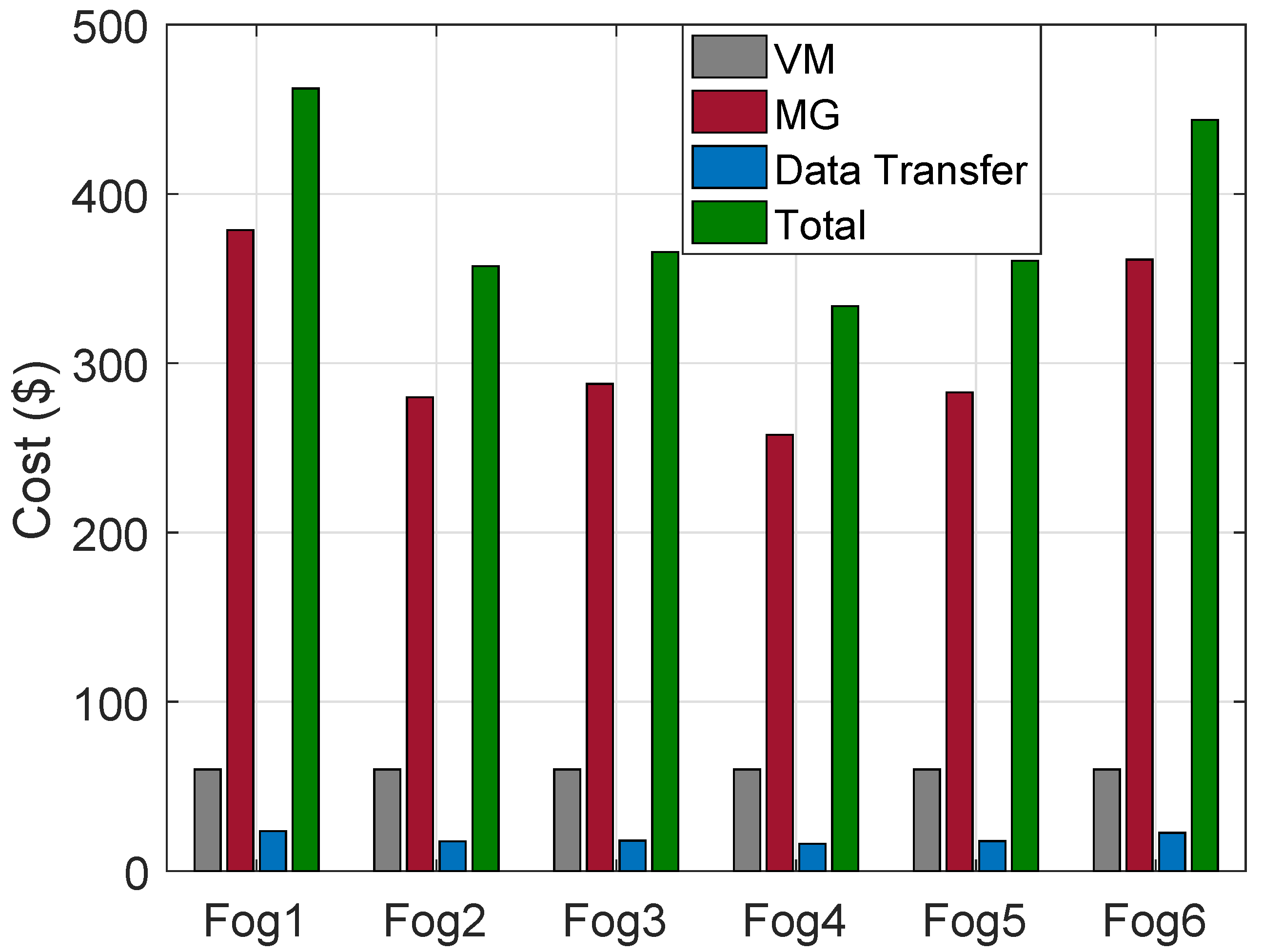
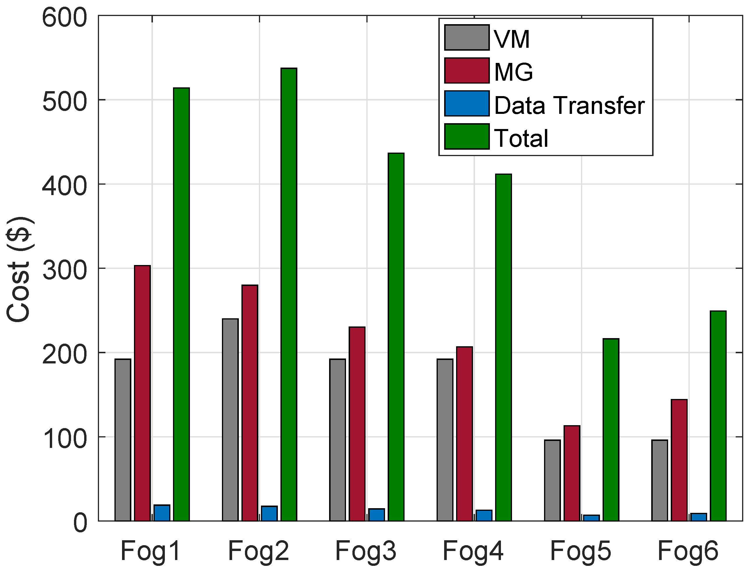
The simulation shows in Figure 3 that total cost of VMs, MGs and DT using ACO and FCFS are the same. The operational cost of each region is associated with MGs, VMs of HPFs and DT. The “Fog4” has the least total cost due to being equivalent to the average number of requests being processed during most of the hours of the day.

The scenario is also implemented in the cloud based system. The cloud has a sum of requests of all HPFs with FCFS and ACO algorithms for allocation of requests to VMs along with ORT service broker policy for selection of data center. In

Table 8. Scenario 1: Response and processing time of cloud.

Time	Load Balancer	Average (ms)	Minimum (ms)	Maximum (ms)
Response	ACO	98.31	69.68	106.62
Processing	ACO	1.12	0.06	2.1
Response	FCFS	101.34	87.02	112.03
Processing	FCFS	1.92	0.10	2.6

, the cloud based system has longer RT as compared to individual HPFs using ACO and FCFS load balancing algorithms. However, PT using ACO is longer as compared to FCFS for the requests of buildings from all the regions. The PT of cloud based system is efficient as compared to individual HPFs. The minimum and maximum RT and PT using ACO and FCFS algorithms are also given in the table. The delayed RT can affect the cost efficiency of energy consumers. For instance, electricity prices are updated at the cloud which may be responded to with a longer delay that compromise the total energy consumption cost for a day. Implementations of cloud based and cloud-fog based systems validate the performance of cloud-fog based system model as well as claim that the SG has time sensitive applications.

5.2. Scenario 2

In this scenario, 50 VMs are considered on HPFs. Huge requests are generated from groups of buildings in the regions and are sent to the HPFs every hour. ACO and FCFS load balancing algorithms allocate the requests on VMs. The RT for the scenario using ACO with average, minimum and maximum are given in

Table 9. Response time of each group of buildings for ACO.

Group of Buildings	Average (ms)	Minimum (ms)	Maximum (ms)
G1	54.52	41.26	67.65
G2	52.18	37.80	65.89
G3	54.57	39.72	70.87
G4	54.50	40.28	70.43
G5	57.50	39.76	78.09
G6	57.83	42.36	75.38

.

Time taken to process requests are also measured in milliseconds. Average, minimum and maximum time for processing of each HPF in a day using ACO algorithm is given in

Table 10. Processing time of each HPF for ACO.

HPF	Average (ms)	Minimum (ms)	Maximum (ms)
HPF1	4.72	0.07	15.57
HPF2	2.54	0.04	10.97
HPF3	4.83	0.07	15.69
HPF4	4.84	0.07	19.34
HPF5	7.70	0.12	27.52
HPF6	8.17	1.05	20.83

.

Unlike $Scenario1$, RT of group of buildings with 50 VMs using FCFS is different from the ACO algorithm. The RT of the number of requests generated every hour from each group of building is given in

Table 11. Response time of each group of buildings for FCFS.

Group of Buildings	Average (ms)	Minimum (ms)	Maximum (ms)
G1	54.29	38.89	67.88
G2	52.01	40.08	67.53
G3	54.48	40.20	69.85
G4	54.31	38.83	67.42
G5	56.78	41.50	70.15
G6	57.12	42.65	70.87

with average, minimum and maximum time.

In the scenario, the number of VMs are twice the amount as compared to $Scenario1$. The number of requests in a day generated from the group of buildings in the regions are processed in respective HPF. Their average, minimum and maximum PT are given in

Table 12. Processing time of each HPF for FCFS.

HPF	Average (ms)	Minimum (ms)	Maximum (ms)
HPF1	4.57	0.07	7.09
HPF2	2.31	0.04	4.95
HPF3	4.65	0.07	7.07
HPF4	4.63	0.07	7.11
HPF5	6.93	0.12	11.00
HPF6	7.39	1.05	10.84

.

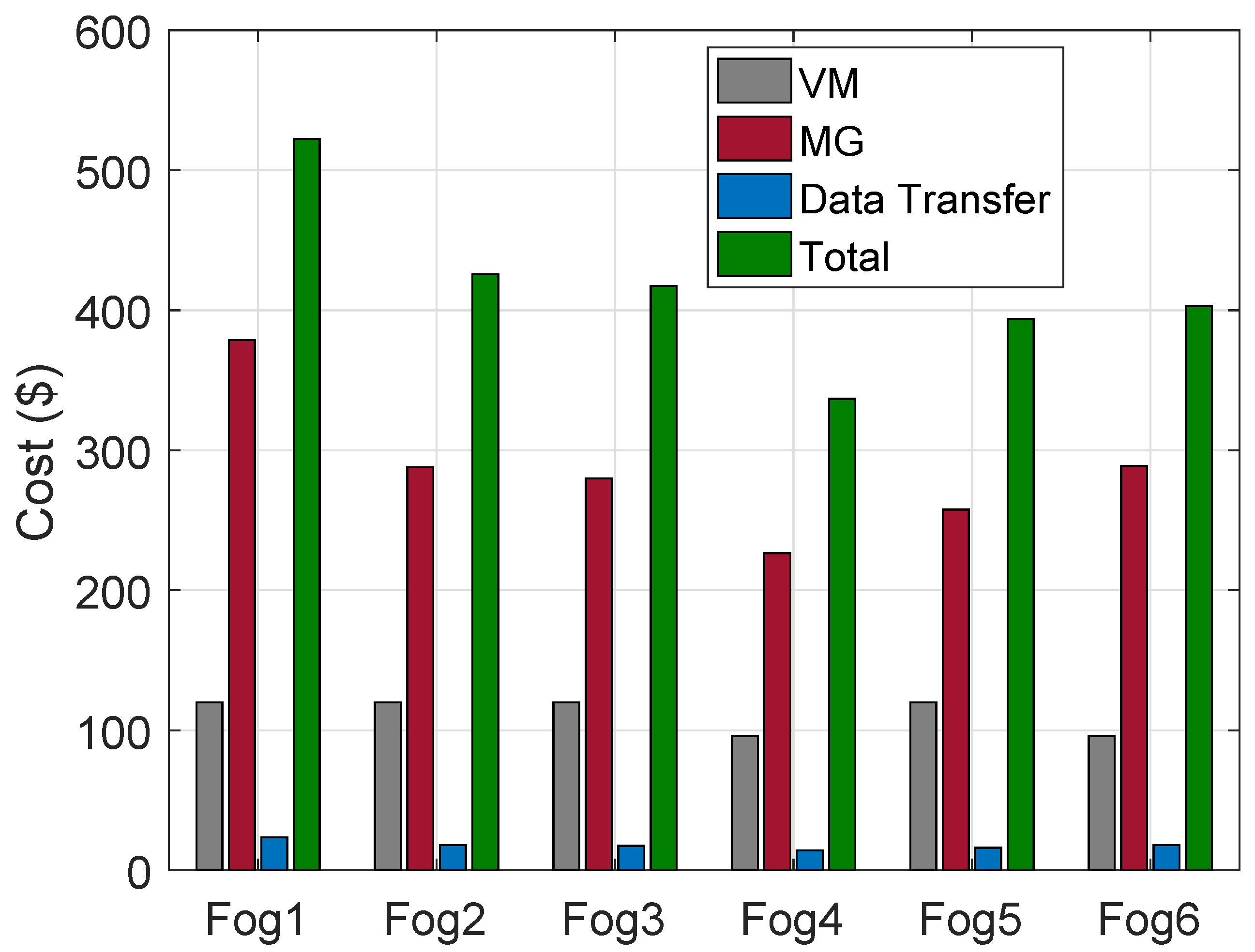
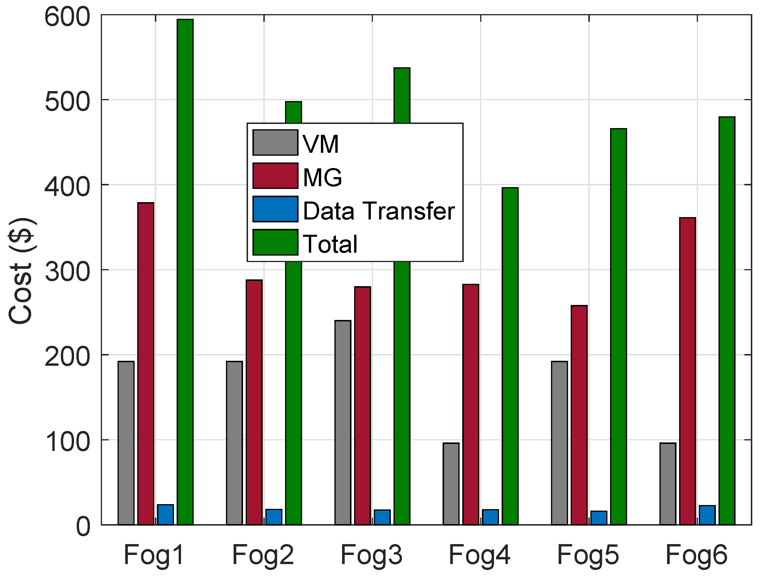
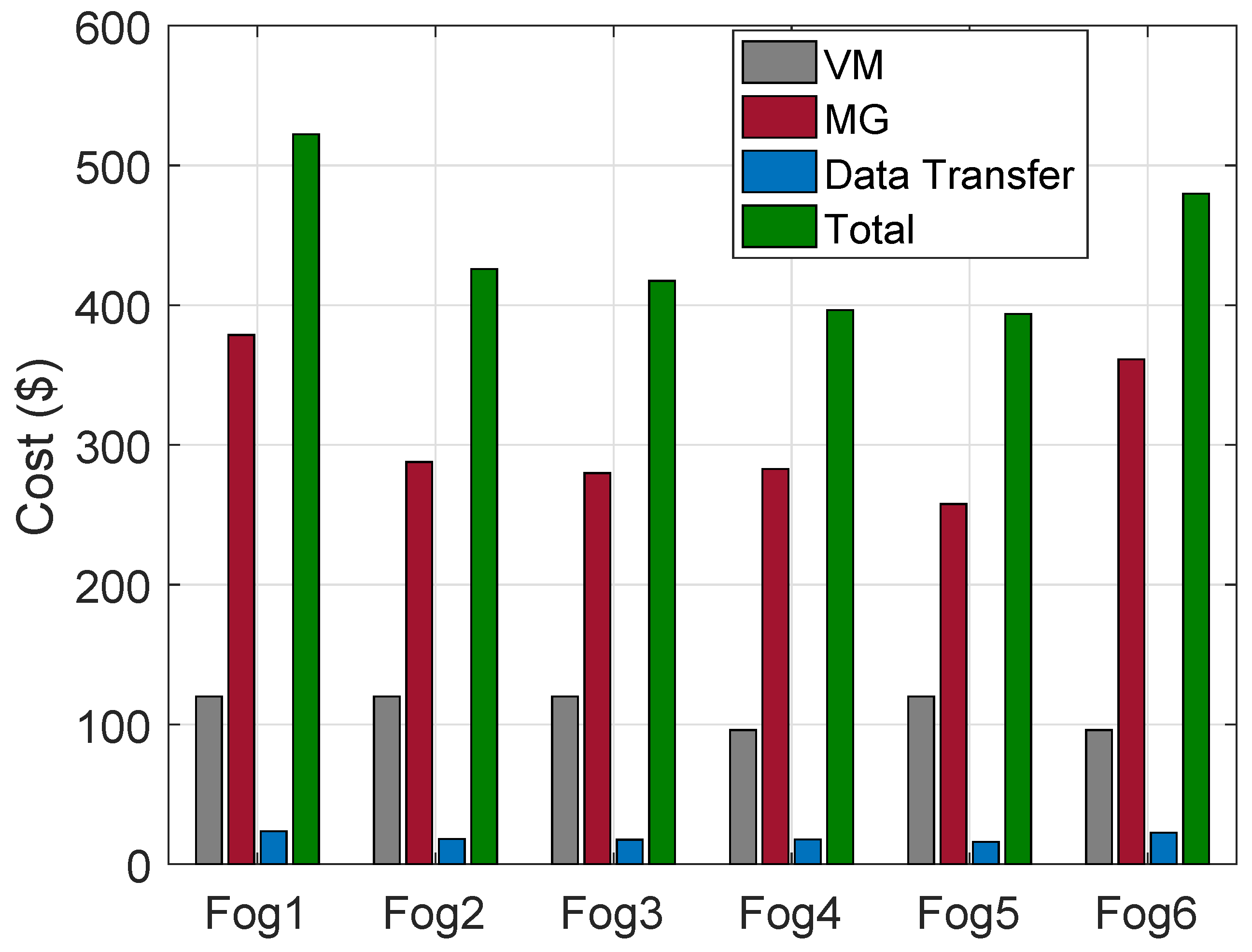
The cost of VMs on HPFs, MGs and DT in the regions are calculated. The cost using ACO is shown in Figure 4. The “Fog4” has the lowest cost due to a lower number of requests being processed as compared to rest of the HPFs in the regions. Similarly, costs of VMs, MGs and DT using FCFS algorithms are shown in Figure 5.

The scenario is also implemented using a cloud based system model. The cloud node has VMs equal to the sum of all VMs on HPFs with the sum of all requests from all the regions. Both FCFS and ACO algorithms are used for allocation of requests to VMs and ORTP is used for data center selection. In Table 8, average RT with ACO algorithm for the cloud based system is longer than HPFs in the regions for the groups of buildings G1, G2, G3, G4, G5 and G6. Each building is entertained with a more delayed response as compared to the cloud-fog based system. Delayed responses for the buildings in the regions compromise the efficiency of energy consumption. For instance, if a building is consuming power with some cost that is updated with cheaper rates; however, delayed response keeps the consumers consume expensive energy for the delayed time. The PT in the cloud is affected with sub-delays like; allocation of requests due to a huge number of requests, evaluation for allocation of requests due to more number of VMs and creation of too many VMs which compromise the performance of physical resources etc. In a cloud based system, average RT and PT using the FCFS algorithm are higher as compared to ACO, which validates the efficiency of ACO. Similarly, variations can be observed for minimum and maximum RT and PT in the table with both ACO and FCFS algorithms. The cloud based system has high processing resources as compared to HPFs that reduce the evaluation time for ACO. Hence, ACO is a good load balancing algorithm; however, time and space complexity is higher as compared to FCFS. The summery of performance with ACO and FCFS is given in

Table 13. Scenario 2: Response and processing time of cloud.

Time	Load Balancer	Average (ms)	Minimum (ms)	Maximum (ms)
Response	ACO	158.01	98.45	172.60
Processing	ACO	2.34	1.0	3.51
Response	FCFS	169.03	101.66	181.53
Processing	FCFS	4.06	2.89	5.99

.

5.3. Scenario 3

In this scenario, the number of VMs are twice the amount as compared to “Scenario 2”. Average, minimum and maximum RT of requests for a group of buildings in a day using ACO are given in

Table 14. Response Ttime of each group of buildings for ACO.

Group of Buildings	Average (ms)	Minimum (ms)	Maximum (ms)
G1	57.44	37.61	77.01
G2	54.17	39.22	69.54
G3	57.58	39.46	81.62
G4	57.53	42.63	73.70
G5	58.63	41.95	81.16
G6	58.90	41.87	83.59

. The PT for the requests of buildings at each HPF for a day using ACO algorithm with average, minimum and maximum are given in

Table 15. Processing time of each group of buildings for ACO.

HPF	Average (ms)	Minimum (ms)	Maximum (ms)
HPF1	7.72	0.11	28.70
HPF2	4.52	0.10	17.16
HPF3	7.83	0.11	29.83
HPF4	7.86	0.11	20.60
HPF5	8.72	0.22	30.33
HPF6	9.16	1.05	30.80

.

The RT for each group of buildings with average, minimum and maximum with the FCFS algorithm on HPFs for a day is given in

Table 16. Response time of each group of buildings for FCFS.

Group of Buildings	Average (ms)	Minimum (ms)	Maximum (ms)
G1	56.77	38.96	71.63
G2	53.69	40.32	69.96
G3	57.02	40.57	73.60
G4	56.82	39.02	71.17
G5	56.78	41.50	70.15
G6	57.12	42.65	70.87

. Similarly, PT for the requests processed at each HPF using the FCFS algorithm for a day with average, minimum and maximum given in

Table 17. Processing time of each group of buildings for FCFS.

HPF	Average (ms)	Minimum (ms)	Maximum (ms)
HPF1	7.05	0.11	10.84
HPF2	4.01	0.06	8.95
HPF3	7.19	0.10	10.82
HPF4	7.15	0.11	10.86
HPF5	6.93	0.12	11.00
HPF6	7.39	1.05	10.84

.

The cost of VMs on HPFs using the ACO algorithm for the allocation of requests of buildings, MGs and DT for a day is shown in Figure 6. The cost of VMs using FCFS algorithm, MGs and DT for a day is shown in Figure 7.

The scenario is also implemented in a cloud based system. The cloud has an equivalent number of VMs as those on all HPFs and the resources. The traffic of requests being routed to the data centers using ORTP and VMs are allocated with requests of buildings from all the regions using ACO as well as FCFS algorithms. The groups of all buildings are connected with the cloud and send a huge number of requests on the cloud for computation. Utility and MGs receive instructions from the cloud.

Table 18. Scenario 3: Response and Processing Time of cloud.

Time	Load Balancer	Average (ms)	Minimum (ms)	Maximum (ms)
Response	ACO	301.01	271.31	324.65
Processing	ACO	4.01	2.01	5.48
Response	FCFS	312.42	288.84	332.10
Processing	FCFS	5.23	3.10	7.21

shows that average RT for groups of buildings in all regions. The ACO is efficient as compared to FCFS algorithm. However, average RT of the cloud is longer than individual HPFs for the group of buildings in the regions which makes the cloud based system inefficient as compared to the HPFs based system. The size of computing resources of the cloud is equivalent to the sum of sizes of the computing resource of all HPFs. The closed based system of $Scenario/2$ is efficient as compared to this scenario due to too many VMs compromising the performance of physical resources of the cloud.

5.4. Comparative Analysis

Three scenarios have been implemented with 25, 50 and 100 VMs on each HPF. The groups of buildings in each region generate a huge number of requests and sent to HPFs. The implementation of the scenarios explained the performance parameters like RT, PT, cost of VMs, MGs and DT. ORTP is implemented for the routing of the requests to data centers. ACO and FCFS algorithms are used for VMs allocation to the requests.

The tables of RT and PT for the requests of buildings for a day with $Scenario1$ have the least values as compared to $Scenario2$ and $Scenario3$ using ACO and FCFS algorithms. VMs are computing resources that enhance the RT and PT by sharing the physical resource; however, too many VMs compromise the performance of physical resources that ultimately compromise the performance of the overall system. Hence, the performances of HPFs and the cloud of $Scenario1$ are ideal as compared to $Scenario2$ and $Scenario3$. The number of VMs of $Scenario2$ are twice the amount of $Scenario1$ and the $Scenario3$ is twice the amount of $Scenario2$. Hence, $Scenario1$ has the ideal number of VMs according to the specification of the physical resource as compared to $Scenario2$ and $Scenario3$. The performances of HPFs and the cloud in the scenarios also affect the depending parameters like the cost of MGs, DT and VMs.

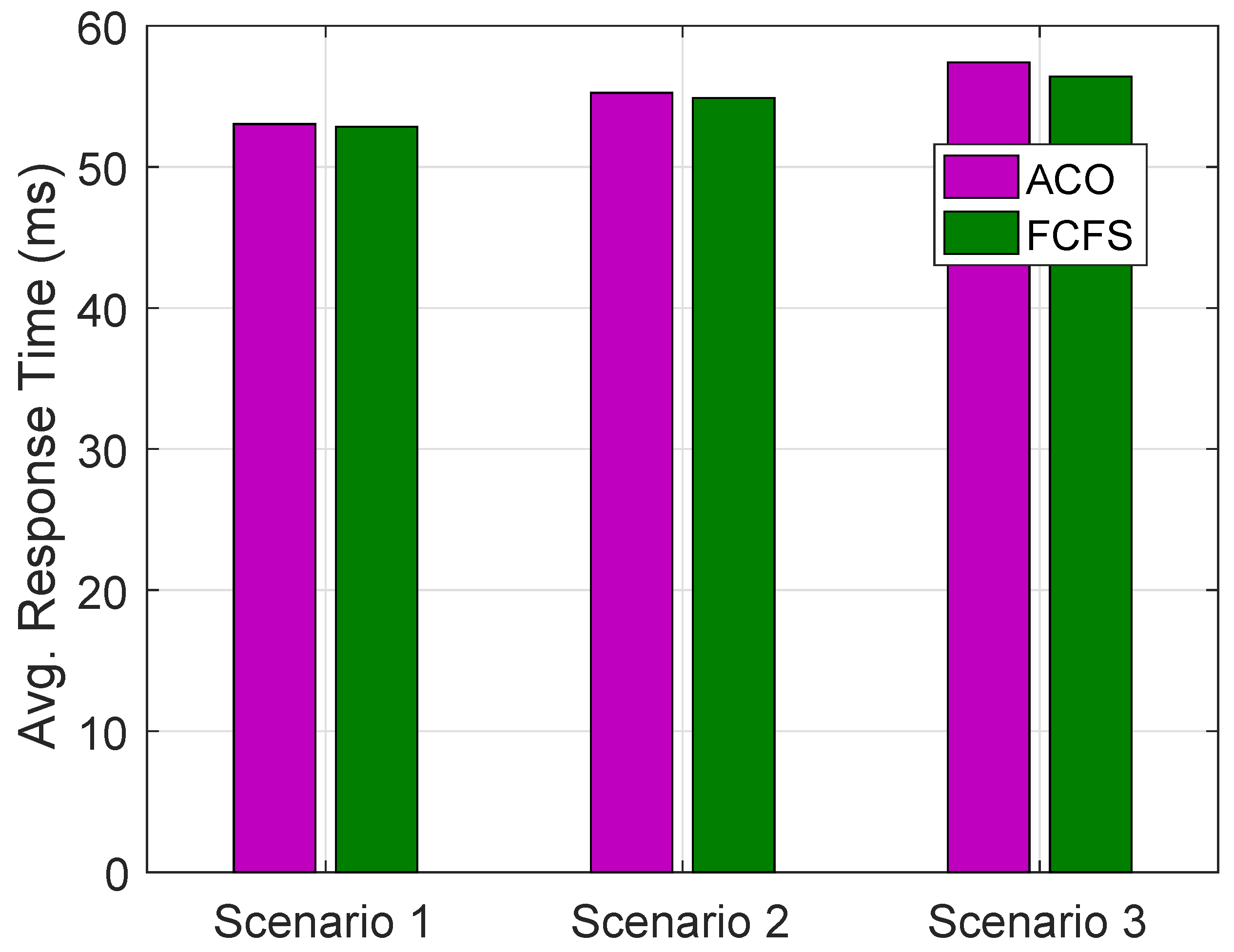
The comparative analysis of all scenarios verifies the claim. In Figure 8, the average PTs for $Scenario1$, $Scenario2$ and $Scenario3$ are given. The RT in $Scenario1$ has less graph representation as compared to $Scenario2$ and $Scenario3$ using ACO and FCFS algorithms for requests of groups of buildings in a day.

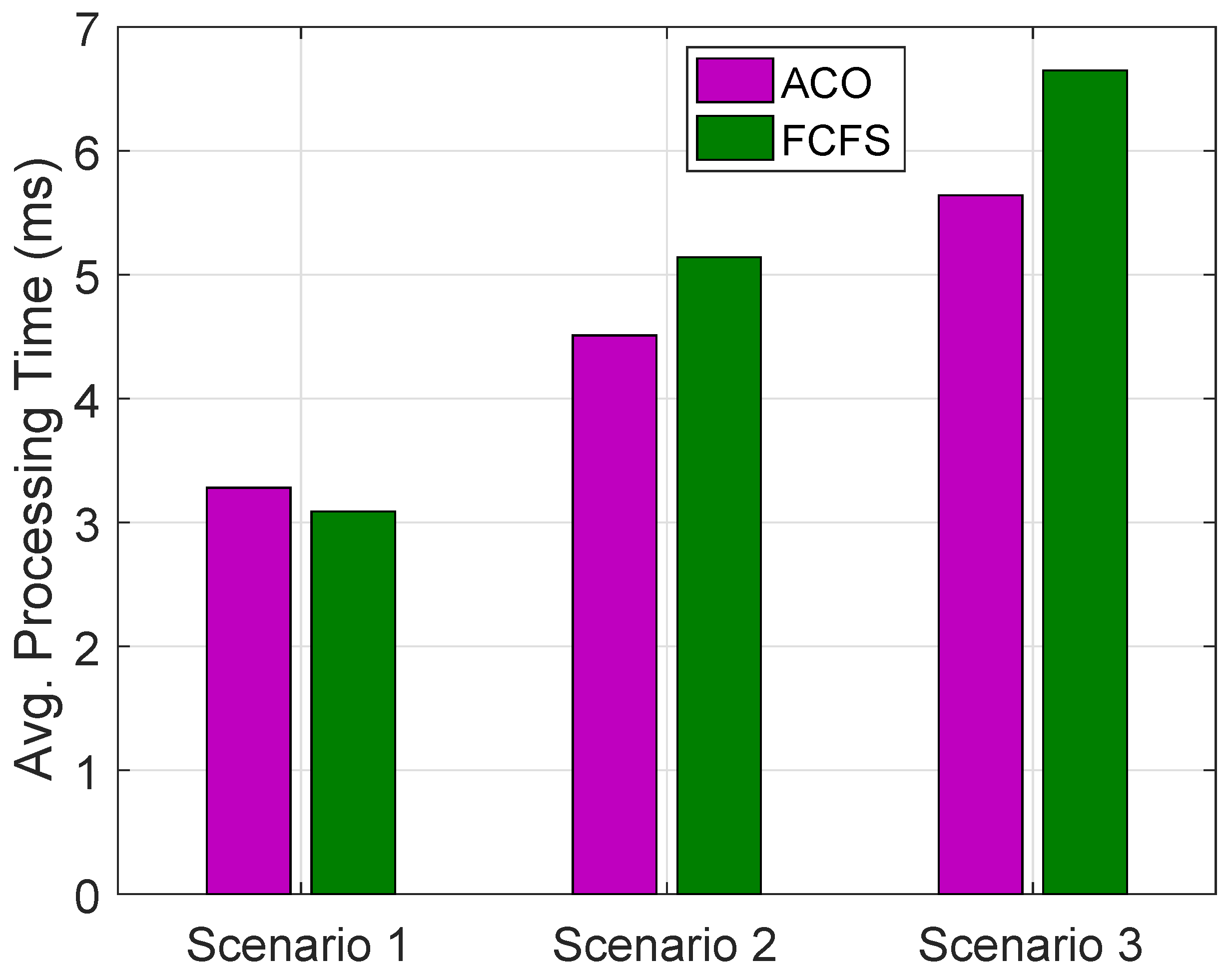
Average PT for all scenarios using ACO and FCFS algorithms for requests of buildings in a day on all HPFs are shown in Figure 9. $Scenario1$ has optimized average PT as compared to $Scenario2$ and $Scenario3$ while $Scenario2$ has optimized PT as compared to $Scenario3$. Average PT using ACO is more optimized then FCFS in $Scenario2$ and $Scenario3$ while this is vice versa in $Scenario1$.

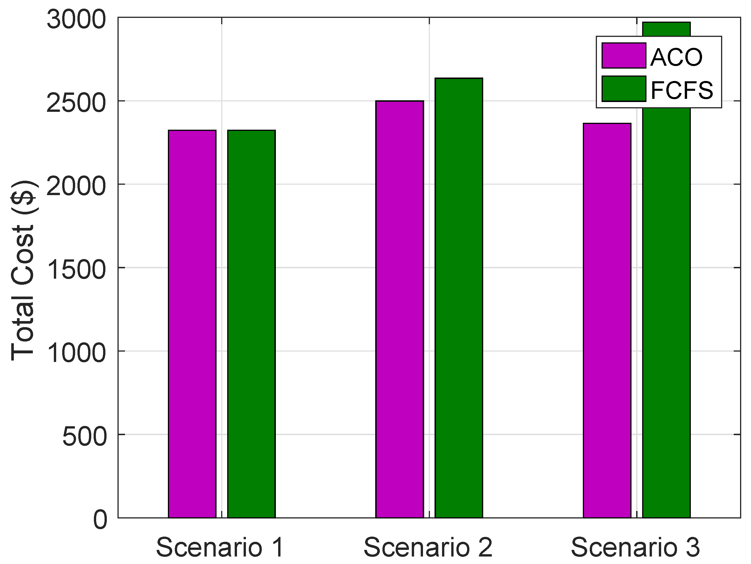
Total cost of VMs, MGs and DT for all scenarios using ACO and FCFS on HPFs for allocation of VMs to the requests of groups of buildings are shown in Figure 10. $Scenario1$ has the lowest cost as compared to $Scenario2$ and $Scenario3$; however, overall cost with ACO is more optimized as compared to FCFS.

The increased number of VMs reduce the RT, PT and increase the cost; however, the simulation results show that RT, PT and cost are increased due to too many virtual resources on physical resources. Hence, too many virtual resources for physical resources compromise the system performance. The average RT and PT of Scenario 2 are longer than Scenario 1, while Scenario 3 has the longest RT and PT with the highest cost. Average RT using ACO of Scenario 3 is increased by 6.70% from $Scenario1$ and 5.05% from $Scenario2$. Similarly, RT using ACO of $Scenario2$ is increased by 1.99% from $Scenario1$. Average RT using FCFS of $Scenario3$ is increased by 3.28%, 4.23% from $Scenario2$ and $Scenario1$, respectively. Similarly, average RT using FCFS of $Scenario2$ is increased by 1.10% from $Scenario1$. Average PT using ACO in $Scenario3$ is increased by 43.87% and 21.07% as compared to $Scenario1$ and $Scenario2$, respectively. Similarly, average PT using FCFS of $Scenario3$ is increased by 54.69% and 23.9% as compared to $Scenario1$ and $Scenario2$, respectively. The cost using ACO for $Scenario2$ is the highest by 8.8% and 4.4% from $Scenario1$ and $Scenario3$. However, using FCFS, the cost in $Scenario3$ is increased by 23.62% and 9.55% from $Scenario1$ and $Scenario2$, respectively. Similarly, cost in $Scenario2$ using FCFS is increased by 15.55% from $Scenario1$. The higher time complexity of ACO is due to the number of iterations performed to find an appropriate solution; hence, ACO is problem-oriented and take a longer time for request allocation and FCFS is simple, timely and an availability based load balancer. Moreover, too many virtual resources on physical resource affect the cost and performance.

The simulations of the scenarios show that cloud-based systems are very slow as compared to the cloud-fog based systems. The cloud based system has 41.72% to 44.14%, 63.40% to 66.98% and 81.71% to 82.81% slower response as compared to the cloud-fog based system in $Scenario1$, $Scenario2$ and $Scenario3$, respectively. Similarly, 46.21% to 49.46%, 66.21% to 69.23% and 81.14% to 82.66% the cloud based system has a slower response as compared to a cloud-fog based system using an FCFS load balancer in $Scenario1$, $Scenario2$ and $Scenario3$, respectively. RT using ACO of $Scenario1$ is 37.78% and 67.38 more efficient as compared to $Scenario2$ and $Scenario3$, respectively, similarly, 40.05% and 67.56% using FCFS. The PT of $Scenario1$ using ACO and FCFS are 52.13% and 52.71% more efficient as compared to $Scenario2$. Similarly, PT using ACO and FCFS of $Scenario1$ are 73.07% and 63.29% more efficient as compared to $Scenario3$.

6. Conclusions and Future Work

In this paper, we have modeled a system in which there are six regions each with a MG, group of buildings of multiple homes and an HPF. MG is used to provide uninterpretable power supply to consumers. Each home generates requests for energy demand and sends to HPF to process. The requests are routed to potential HPF using ORTP service broker policy and assigned to the corresponding VM using either ACO or FCFS load balancing algorithms. The RT and PT of requests from each region are optimized using aforementioned service broker policy and load balancing algorithms. Three scenarios with 25, 50 and 100 VMs are implemented to analyse the effects on RT, PT and cost. RT and PT in Scenario 1 are more optimized as compared to $Scenario2$ and $Scenario3$; however, $Scenario2$ has twice the number of VMs as compared to $Scenario1$ and $Scenario3$ has twice the number of VMs as compared to $Scenario2$. VMs are installed on physical resources for resource sharing. Simulations validate that physical resources are suffocated when VMs are increased beyond their limits. $Scenario1$ has 25 VMs that are suitable for physical resource sharing while 50 and 100 VMs in $Scenario2$ and $Scenario3$ share the physical resources more than the capacity, which slows down the system by affecting the parameters like RT, PT and cost. Cloud based system has longer delay issues that does not suit SG such as time sensitive applications.The simulation results prove that the cloud-fog based system shows high performance as compared to only fog based system for time sensitive SG applications. Moreover, too many VMs with respect to capacity of physical resources compromise the RT, PT and the cost. In $Scenario1$, fogs have less VMs than $Scenario2$ and $Scenario3$; therefore, performance of $Scenario1$ is better as compared to the other two scenarios. There are too many VMs in $Scenario2$ and $Scenario3$ for physical resources.

In the future, we will provide a mathematical and logical evaluation criterion to create a suitable number of VMs on physical systems for efficient performance.

References

1. Aslam, S.; Iqbal, Z.; Javaid, N.; Khan, Z.A.; Aurangzeb, K.; Haider, S.I. Towards efficient energy management of smart buildings exploiting heuristic optimization with real-time and critical peak pricing schemes. Energies 2017, 10, 2065. [Google Scholar] [CrossRef]
2. Baalamurugan, K.M.; Bhanu, D.S.V. Analysis of Cloud Storage Issues in Distributed Cloud Data Centres by Parameter Improved Particle Swarm Optimization (PIPSO) Algorithm. Int. J. Future Revolut. Comput. Sci. Commun. Eng. 2018, 4, 303–307. [Google Scholar]
3. Sadiku, M.N.; Musa, S.M.; Momoh, O.D. Cloud computing: Opportunities and challenges. IEEE Potentials 2014, 33, 34–36. [Google Scholar] [CrossRef]
4. Fatima, I.; Javaid, S.; Javaid, N.; Shafi, I.; Nadeem, Z.; Ullah, R. Region Oriented Integrated Fog and Cloud Based Environment for Efficient Resource Distribution in Smart Buildings. In Proceedings of the Conference on Complex, Intelligent, and Software Intensive Systems, Matsue, Japan, 4–6 July 2018; Springer: Cham, Switzerland; pp. 749–759. [Google Scholar]
5. Manasrah, A.M.; Ba Ali, H. Workflow scheduling using hybrid GA-PSO algorithm in cloud computing. Wirel. Commun. Mob. Comput. 2018, 2018, 1934784. [Google Scholar] [CrossRef]
6. Pham, N.M.N.; Le, V.S. Applying Ant Colony System algorithm in multi-objective resource allocation for virtual services. J. Inf. Telecommun. 2017, 1, 319–333. [Google Scholar] [CrossRef]
7. Cao, Z.; Lin, J.; Wan, C.; Song, Y.; Zhang, Y.; Wang, X. Optimal cloud computing resource allocation for demand side management in smart grid. IEEE Trans. Smart Grid 2017, 8, 1943–1955. [Google Scholar]
8. Khalid, A.; Javaid, N.; Guizani, M.; Alhussein, M.; Aurangzeb, K.; Ilahi, M. Towards dynamic coordination among home appliances using multi-objective energy optimization for demand side management in smart buildings. IEEE Access 2018, 6, 19509–19529. [Google Scholar] [CrossRef]
9. Bera, S.; Misra, S.; Rodrigues, J.J. Cloud computing applications for smart grid: A survey. IEEE Trans. Parallel Distrib. Syst. 2015, 5, 1477–1494. [Google Scholar] [CrossRef]
10. Li, D.; Hong, P.; Xue, K.; Pei, J. Virtual Network Function Placement Considering Resource Optimization and SFC Requests in Cloud Datacenter. IEEE Trans. Parallel Distrib. Syst. 2018, 29, 1664–1677. [Google Scholar] [CrossRef]
11. Shih, P.J. From the Cloud to the Edge: The Technical Characteristics and Application Scenarios of Fog Computing. Int. J. Autom. Smart Technol. 2018, 8, 61–64. [Google Scholar] [CrossRef]
12. Xue, K.; Hong, J.; Ma, Y.; Wei, D.S.; Hong, P.; Yu, N. Fog-Aided Verifiable Privacy Preserving Access Control for Latency-Sensitive Data Sharing in Vehicular Cloud Computing. IEEE Netw. 2018, 32, 7–13. [Google Scholar] [CrossRef]
13. Wang, P.; Chen, X.; Sun, Z. Performance Modeling and Suitability Assessment of Data Center Based on Fog Computing in Smart Systems. IEEE Access 2018, 99, 1. [Google Scholar] [CrossRef]
14. Shabeera, T.P.; Kumar, S.M.; Salam, S.M.; Krishnan, K.M. Optimizing VM allocation and data placement for data-intensive applications in cloud using ACO metaheuristic algorithm. Eng. Sci. Technol. Int. J. 2017, 20, 616–628. [Google Scholar] [CrossRef]
15. Wickremasinghe, B.; Buyya, R. CloudAnalyst: A CloudSim-based tool for modelling and analysis of large scale cloud computing environments. MEDC Proj. Rep. 2009, 22, 433–659. [Google Scholar]
16. Shaw, S.B. Balancing Load of Cloud Data Center using Efficient Task Scheduling Algorithm. Int. J. Comput. Appl. 2017, 159, 1–5. [Google Scholar]
17. Bhole, R.; Singh, H.J.; Khamkar, P.; Joshi, P.; Bendbhar, R. Load Balancing in Cloud Computing Using Autonomous Agents. Imp. J. Interdiscip. Res. 2017, 3, 237–239. [Google Scholar]
18. Mohanty, S.; Patra, P.K.; Ray, M.; Mohapatra, S. A Novel Meta-Heuristic Approach for Load Balancing in Cloud Computing. Int. J. Knowl.-Based. Organ. 2018, 8, 29–49. [Google Scholar] [CrossRef]
19. Tiwari, P.K.; Joshi, S. Effective Management of Data Centers Resources for Load Balancing in Cloud Computing. Int. J. Inf. Retr. Res. 2018, 8, 40–56. [Google Scholar] [CrossRef]
20. Sultanpure, K.A.; Reddy, L.S.S. An Energy Aware Resource Utilization Framework to Control Traffic in Cloud Network and Overloads. Int. J. Electr. Comput. Eng. 2018, 8, 1018–1027. [Google Scholar] [CrossRef] [Green Version]
21. Chen, S.L.; Chen, Y.Y.; Kuo, S.H. CLB: A novel load balancing architecture and algorithm for cloud services. Comput. Electr. Eng. 2017, 58, 154–160. [Google Scholar] [CrossRef]
22. Moghaddam, M.H.Y.; Leon-Garcia, A.; Moghaddassian, M. On the performance of distributed and cloud-based demand response in smart grid. IEEE Trans. Smart Grid 2017. [Google Scholar] [CrossRef]
23. Razzaghzadeh, S.; Navin, A.H.; Rahmani, A.M.; Hosseinzadeh, M. Probabilistic modeling to achieve load balancing in Expert Clouds. Ad Hoc Netw. 2017, 59, 12–23. [Google Scholar] [CrossRef]
24. Chugh, S.; Verma, A.; Sharma, K.; SSIET, D. Data Center Processing Time Evaluation of Service Broker Policies In A single Data Center. Available online: http://oaji.net/articles/2015/786-1440846326.pdf (accessed on 12 March 2018).
25. Mohamed, N.; Al-Jaroodi, J.; Jawhar, I.; Lazarova-Molnar, S.; Mahmoud, S. SmartCityWare: A Service-Oriented Middleware for Cloud and Fog Enabled Smart City Services. IEEE Access 2017, 5, 17576–17588. [Google Scholar] [CrossRef]
26. Chekired, D.A.; Khoukhi, L.; Mouftah, H.T. Decentralized Cloud-SDN Architecture in Smart Grid: A Dynamic Pricing Model. IEEE Trans. Ind. Inform. 2018, 14, 161–169. [Google Scholar] [CrossRef]
27. Islam, N.; Waheed, S. Fuzzy based Efficient Service Broker Policy for Cloud. Int. J. Comput. Appl. 2017, 168, 3740. [Google Scholar] [CrossRef]
28. Anderson, D.; Gkountouvas, T.; Meng, M.; Birman, K.; Bose, A.; Hauser, C.; Zhang, F. GridCloud: Infrastructure for Cloud-based Wide Area Monitoring of Bulk Electric Power Grids. IEEE Trans. Smart Grid 2018. [Google Scholar] [CrossRef]
29. Lyu, L.; Nandakumar, K.; Rubinstein, B.; Jin, J.; Bedo, J.; Palaniswami, M. PPFA: Privacy Preserving Fog-enabled Aggregation in Smart Grid. IEEE Trans. Ind. Inform. 2018, 14, 3733–3744. [Google Scholar] [CrossRef]
30. Hussain, M.; Alam, M.S.; Beg, M.M. Fog Computing in IoT Aided Smart Grid Transition-Requirements, Prospects, Status Quos and Challenges. arXiv 2018, arXiv:1802.01818. [Google Scholar]
31. He, D.; Kumar, N.; Zeadally, S.; Wang, H. Certificateless Provable Data Possession Scheme for Cloud-Based Smart Grid Data Management Systems. IEEE Trans. Ind. Inform. 2018, 14, 1232–1241. [Google Scholar] [CrossRef]
32. Capizzi, G.; Sciuto, G.L.; Napoli, C.; Tramontana, E. Advanced and Adaptive Dispatch for Smart Grids by means of Predictive Models. IEEE Trans. Smart Grid 2017. [Google Scholar] [CrossRef]
33. Al Faruque, M.A.; Vatanparvar, K. Energy management-as-a-service over fog computing platform. IEEE Internet Things J. 2016, 3, 161–169. [Google Scholar] [CrossRef]
34. Shojafar, M.; Cordeschi, N.; Baccarelli, E. Energy-efficient adaptive resource management for real-time vehicular cloud services. IEEE Trans. Cloud Comput. 2016, 1–14. [Google Scholar] [CrossRef]
35. Pooranian, Z.; Shojafar, M.; Naranjo, P.G.V.; Chiaraviglio, L.; Conti, M. A novel distributed fog-based networked architecture to preserve energy in fog data centers. In Proceedings of the IEEE 14th International Conference on Mobile Ad Hoc and Sensor Systems (MASS), Orlando, FL, USA, 22–25 October 2017; pp. 604–609. [Google Scholar]
36. Baccarelli, E.; Naranjo, P.G.V.; Scarpiniti, M.; Shojafar, M.; Abawajy, J.H. Fog of everything: Energy-efficient networked computing architectures, research challenges, and a case study. IEEE Access 2017, 5, 9882–9910. [Google Scholar] [CrossRef]
37. Patel, H.; Patel, R. Cloud Analyst: An Insight of Service Broker Policy. Int. J. Adv. Res. Comput. Commun. Eng. 2015, 4, 122–127. [Google Scholar] [CrossRef]
38. Ismkhan, H. Effective heuristics for ant colony optimization to handle large-scale problems. Swarm Evol. Comput. 2017, 32, 140–149. [Google Scholar] [CrossRef]
Figure 1. Proposed system model.
Sustainability 10 03592 g001
Figure 2. Amount of request load on each HPF.
Sustainability 10 03592 g002
Figure 3. VM, MG, DT and total cost for ACO or FCFS.
Sustainability 10 03592 g003
Figure 4. VM, MG, DT and total cost for ACO.
Sustainability 10 03592 g004
Figure 5. VM, MG, DT and total cost for FCFS.
Sustainability 10 03592 g005
Figure 6. VM, MG, DT and total cost for ACO.
Sustainability 10 03592 g006
Figure 7. VM, MG, DT and total cost for FCFS.
Sustainability 10 03592 g007
Figure 8. Response time comparison between ACO and FCFS for all scenarios.
Sustainability 10 03592 g008
Figure 9. Processing time comparison between ACO and FCFS for all scenarios.
Sustainability 10 03592 g009
Figure 10. Total cost comparison between ACO and FCFS for all scenarios.
Sustainability 10 03592 g010