The Dual Threshold Limit of Financing and Formal Credit Availability with Chinese Rural Households: An Investigation Based on a Large Scale Survey

Abstract

The literature on credit availability for rural households primarily focuses on the supply side, and largely ignores the demand side. This paper divided the credit process into three stages using large-scale household survey data. It also reviewed the credit process in other developing countries. A dual sample selection model was used to deal with the dual self-selection problem, which has been neglected in previous studies. This paper found that the main obstacle that farmers faced in obtaining financing was fear of applying for credit from formal financial institutions. In addition, there were significant differences in the determinants of different stages of the credit process of rural households.

1. Introduction

Rural financial markets are key elements of solutions to rural problems. Promoting rural financial reform and building a new rural financial system is one of the key factors for achieving sustainable economic and social development. Rural credit is an indispensable factor in the capital movement in the process of agricultural reproduction. It is an important link in raising and regulating agricultural funds, and an important channel for the country to support agriculture. It is of great significance for promoting the consolidation and development of socialist production relations in agriculture and promoting the realization of agricultural modernization.

Therefore, the Chinese government has attached great importance to the construction and improvement of the rural financial system over the years. The central government has also devoted much effort to improving the rural financial system. Because of the long-term existence of financing difficulties in rural areas, the structure of farmers’ credit constraints has changed significantly. It has shifted from simple supply constraints to hybrid credit constraints that are intertwined with the supply side [1]. Furthermore, when farmers have credit demands, they must break the double threshold between the demand side and the supply side; they must overcome both the demand-based constraints caused by credit panic and the supply type constraints of financial institutions caused by credit behavior [1,2]. However, rural financial reform has largely been directed at the credit supply and the reform and reconstruction of the rural financial system. Thus, demand has received insufficient attention, which has impacted the practical effects of rural financial reform, and farmers still suffer from widespread financing dilemmas [3,4,5,6]. At present, China’s rural financial reform is in the deepening stage. One of its important goals is to find a path through the double threshold of financing and improve credit availability to farmers. Therefore, understanding the credit process of farmers is crucial.

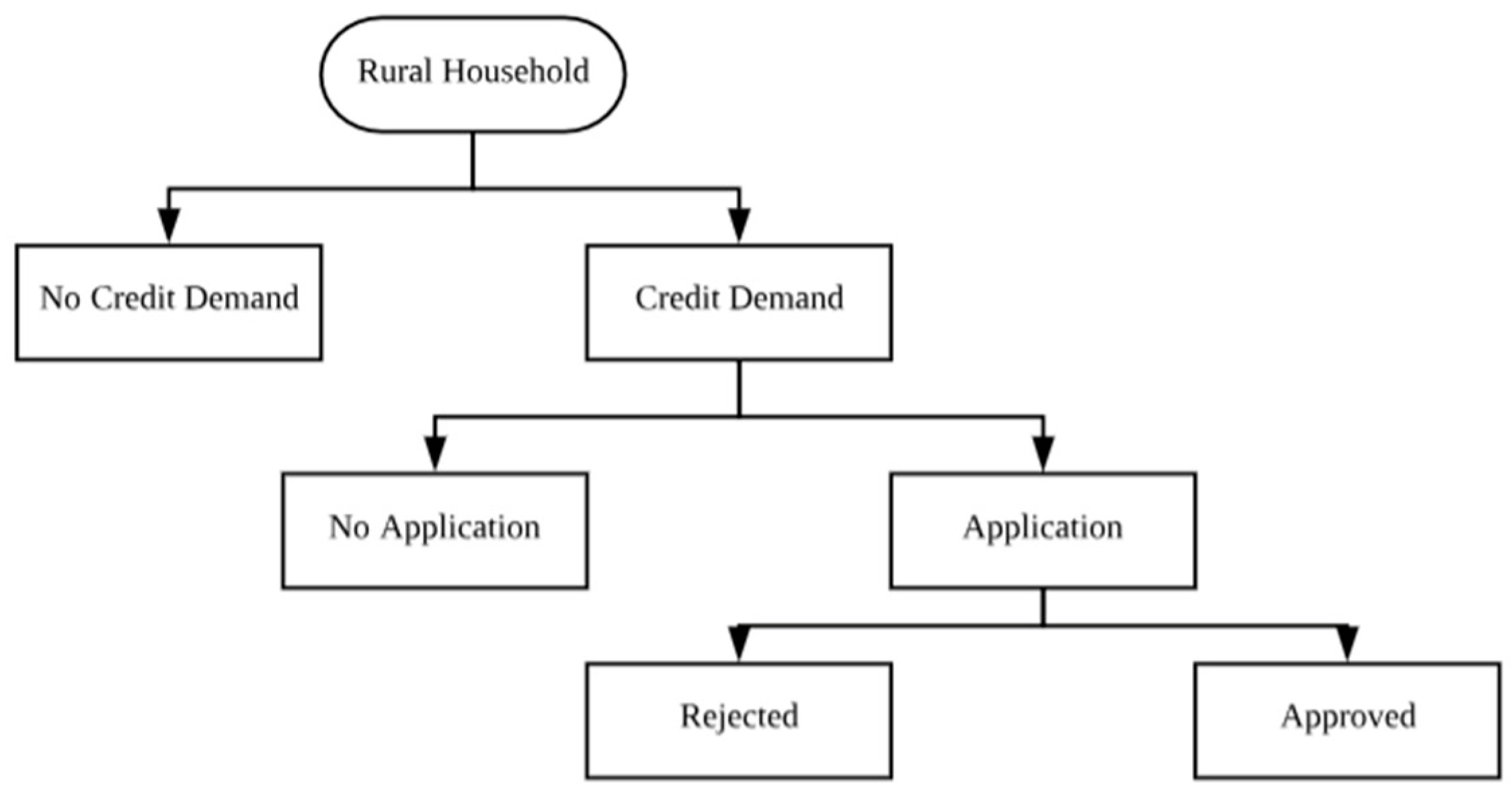
The credit process of farmers can be divided into three stages. Stage one is credit demand. The sample of all households can be divided into two categories based on whether they have credit demand. Stage two is credit application. The houses can then be further divided into two types based on whether they have applied for credit. In stage three, households applying for credit are divided into two groups based on whether the application is approved.

As shown in Figure 1, we can observe credit applications only if there is a credit demand, and we can observe credit availability status only if there is an application. In this simple chain of logic, each level is conditional on the previous one. Thus, samples are not randomly chosen, but are instead selected. In this case, even with a random sampling method, there is a sample selection bias problem, which leads to bias in the estimation results [7]. Therefore, based on the three-stage model of rural household credit, analyses of the availability of rural credit are shaped by both the sample selectivity of credit demand and the sample selectivity of credit application. We call this the “double sample selectivity problem” of the credit process.

To explore the affecting factors in different stages of the household credit process, most studies conduct field investigations through direct heuristics and then construct econometric models for identification. However, the literature focuses on a single sample selectivity problem and ignores the double sample selectivity problem. For example, Yang et al., Zhang Bing and Zhang Ning, Liu Xichuan et al. [8,9,10,11] and other researchers use econometric models such as Tobit II or Tobit III to integrate farmers’ credit demand and the credit scale into the same framework. The shortcoming of this literature is that they did not consider the intermediate stage of the credit process, i.e., the credit application, by only considering the sample selection of credit demand. The sample selection problem of credit application was ignored. Liu Xichuan et al. [12] developed the Quaternary-dimensional Probit Model with sample selectivity (hereinafter referred to as the QPM model) to incorporate the credit demand and credit availability from formal and informal financial channels within the same framework. Though the credit behavior and interactions between different channels was considered, it neglected the sample selection bias problem. Zhang Ning and Zhang Bing [13] established a two-variable Probit model based on sample selectivity (BPSS model) to consider credit application amount and bank credit approval amount in the same framework for analysis. However, this method did not consider the initial stages of the credit process, i.e., whether there is credit demand, instead exploring only the credit application sample selection. Li Qinghai et al. [1,14] constructed a dual sample selection model (DSS model) to examine the dual sample selectivity problem in the credit process, the sample was limited to the Shandong and Jiangsu provinces, and the conclusions obtained were not representative of the whole country. Hence, it lacks the external validity necessary for policy recommendations. Therefore, to identify factors affecting the household credit process, especially the credit availability, it is necessary to introduce new econometric models.

This paper uses the large sample micro-survey data of the People’s Bank of China, combined with the dual sample selection model, to examine the factors affecting the credit process, especially credit availability.

This paper makes the following contributions:

(1)

Research ideas. This paper constructs a simultaneous equation model and integrates the three stages of the household credit process, i.e., credit demand, credit application, and credit availability, into the same framework to prevent information loss in the sample.

(2)

Econometric model. This paper chooses the double sample selection model for analysis, which effectively solves the double sample selection bias caused by credit demand and application.

(3)

Data. This paper uses a large number of data samples. A total of 20,000 farmer households in 236 counties in 10 provinces or cities across the country have been collected, representing the demographic widely and well.

The remainder of the paper is organized as follows. The second section presents the literature review. Section three establishes a dual sample selection model to incorporate the three stages of the household credit process into the same the framework to address the double sample selectivity problem caused by credit demand and application. In addition, also explains the variable selection. Section five describes the results. The final section summarizes the research conclusions and proposes policy recommendations. It also presents the limitations and future research areas.

2. Literature Review

Analysis the current rural household credit status takes an important part for the rural financial system reform. Researchers in China and other counties studied the rural household credit access problem from different angles and used various methods. Yin Haodong et al. [15] studied the replacement effect between formal institutional credit and informal rural credit channel using a linear regression model based on a survey of 2085 samples. It arrived at the conclusion that informal channels could satisfy most credit demands. Farmers have constraints in applying for credit from formal channels. Wu Yu et al. [16] used an instrument variable model and Heckman Probit model to study the factors affecting the rural household, choosing different channels by using data of the China Household Finance Survey in 2013. Changsheng Li et al. [17] used two instrument variables to explore the impact of credit constraints on rural households’ consumption expenditure in south China based on a random survey of 918 rural households in Jiangxi province.

Improving rural household credit access is a major issue for rural finance reform in other developing countries, as well. Many researchers analyzed the credit access limit and how informal and formal credit channels interactively affect the rural financial system. Anjani Kumar et al. [18] used large national farm household level data and IV 2SLS estimation methods to investigate the role of institutional farm credit on farm income and farm household consumption expenditures in India. They arrived at the conclusion that formal credit plays an important role in improving farm income in India. Mikkel Barslund et al. [19] used a survey of 932 rural households to uncover how the rural credit market operates in Vietnam. They concluded that credit rationing depends on education and credit history. A probit model was used to describe the demand for credit. Diagne Aliou et al. [20] measured the level of household access to credit of Malawi and Bangladesh. They corrected the shortcomings of the traditional methodology when detecting the credit constraints, as well as the direct household survey, by developing a conceptual framework and data collection methodology focusing on the concept of credit limit. Msoo A. et al. [21] used the OLS model to analyze the welfare effect of diversification in Nigeria.

Although there is increasing attention in social and academic circles to the credit process of rural households, and numerous studies have been conducted, researchers have seldom included the three stages of the rural credit process in the same framework for analysis. In general, research on the factors influencing the different stages of the household credit process can be divided into the two types discussed below.

2.1. No Consideration of the Interrelationship between Different Stages of the Household Credit Process

Researchers have often considered the different stages of the credit process—credit demand, application, and availability—as separate processes, and then separately identified the factors influencing each stage. Their results appear to suffer from sample selectivity bias.

To explore credit demand and applications, researchers have primarily used the Probit/Logit model for analysis. For example, Wang Changyun et al. [22] used the Probit model to identify the factors influencing credit demand. Lin Lefen and Yu Yuxi [23] used the Logit model for analysis. Yi Xiaolan [24] used the Logit model to identify the factors affecting rural households credit applications to formal financial institutions. Jin Han and Li Hongbin [25] used two independent Logit models to identify and compare the factors influencing and differences between rural formal and informal channel credit applications.

Research into credit availability can be divided into two sub-categories based on whether credit is sought. Common models include:

(1)

Probit/Logit model. Tong Xinle et al. [26] used a Logit model to identify factors affecting credit approval. Similar analyses have been performed by Hu Lian et al. [27] and Xu Lihe and Yuan Yan [28].

(2)

Multi-Probit/Logit model. Feng Xufang [29] and Chu Baojin [30] classified rural households into four categories: having no credit demand, using informal credit channels, using formal credit channels, and using both formal and informal credit channels. A multivariate Logit model was used to examine and compare the factors affecting the formal and informal channel usage of rural households. Zhang Bing and Zhang Ning [9] regarded each type of credit as a case, and divided the sample into three categories: zero-interest informal credit, high-interest informal credit, and formal credit, and used a multivariate Logit model in their analysis.

(3)

Ordered Probit/Logit model. Zhang Bing et al. [13] used an ordered Logit model and divided farmers into four categories: non-credit demand, informal channel, semi-formal channel, and formal channel.

(4)

Bivariate Probit model (Biprobit model). Zhou Tianyi and Li Jie [31] and Hu Feng and Chen Yuyu [32] used a Biprobit model to analyze the interaction between formal and informal channels, while identifying the factors affecting the availability of credit from the formal and informal channels.

(5)

DSS Model. Li Qinghai et al. [14] constructed a dual sample selection model to identify the factors affecting credit demand, application, and approval, and incorporated the credit process into the same framework for analysis.

Another type of analysis explores the credit scale, using models such as:

(1)

OLS model. Tong Xinle et al. [26] used multiple linear regression models to identify the factors influencing the actual credit amount of farmers.

(2)

Tobit I model. Yi Xiaolan [24] used this model to identify the factors affecting the formal credit availability by measuring the actual ratio of credit approval amount over application amount. Wang Changyun et al. [22] used this model to formalize rural households and identify factors influencing the credit scale. Jin Han and Li Hongbin [33] and Hu Feng and Chen Yuyu [32] used two independent Tobit I models to identify the factors affecting the scale of rural formal and informal financial channels.

(3)

Simultaneous Binary Tobit I model (Bitobit model). He Guanghui and Yang Xianyue [34] adopted this model to analyze the interaction between formal and informal financial channels, and identify the factors affecting the amount approved by different channels.

2.2. Consider the Interaction between Different Stages of the Rural Household Credit Process

Many studies have considered the correlations between different stages of the household credit process, and constructed simultaneous equation models for analysis, largely Tobit II models [8,10,11,12], Tobit III models [10], BPSS model [13] and QPM with sample selectivity [11]. However, as mentioned above, these studies often only consider two stages of the credit process, such as credit demand and credit availability [8,10,11,12]. Therefore, they do not address the sample selection problem in credit application. Thus, new econometric models that can correctly identify the factors influencing the different stages of the rural household credit process are necessary.

3. The Econometric Model

3.1. Dual Sample Selection Model

When analyzing the credit availability of rural households, if the double sample selectivity problem is not addressed, estimation bias may occur. Hence, this paper constructs a dual sample selection model with three-stage simultaneous equations to correct the estimation bias caused by double sample selectivity [35,36,37]. Since considering credit from informal channels will lead to analytical difficulty, this paper considers only the credit availability from formal channels. Drawing on the ideas of Vadean and Piracha [35], the dual sample selection model for identifying the factors influencing the different stages of the household credit process is as follows:

$$L{D}^{*}=X_1^{’}{\beta }_1+{\epsilon }_1, LD=I \left(L{D}^{*}>0\right)$$

(1)

$$L{A}^{*}=X_2^{’}{\beta }_2+{\epsilon }_2, LA=I \left(L{A}^{*}>0\right), if LD=1$$

(2)

$$L{R}^{*}=X_3^{’}{\beta }_3+{\epsilon }_3, LR=I \left(L{R}^{*}>0\right), if LD=1 and LA=1$$

(3)

where $\left(X_1,X_2,X_3\right)$ satisfies $\left(X_1\ne X_2\ne X_3\right)$, $\left(L{D}^{*},L{A}^{*},L{R}^{*}\right)$ represents potential results, and $I(·$) represents the binary exponential function. Where $\left({\epsilon }_1,{\epsilon }_2,{\epsilon }_3\right)\in N \left(0,V\right)$, V is a symmetric matrix, for ${\epsilon }_k,{\epsilon }_l\in \left({\epsilon }_1,{\epsilon }_2,{\epsilon }_3\right)$ ($k\ne$l), the correlation coefficient for errors satisfies ${\rho }_{lk}={\rho }_{kl},{\rho }_{kk}=1$, and the errors $\left({\epsilon }_1,{\epsilon }_2,{\epsilon }_3\right)$ in the simultaneous Equations are orthogonal with $\left(X_1,X_2,X_3\right)$.

According to the simultaneous Equations (1)–(3), the data can be divided into four mutually exclusive categories: (1) no credit demand where $LD=0$; (2) there is demand but no credit application, where $LD=1,LA=0$; (3) there is credit demand and application for credit, but the credit is not obtained, where $LD=1,LA=1,LR=0$; and (4) there is demand and credit is obtained after application, where $LD=1,LA=1,LR=1$. The sum of the probabilities of the four categories equals 1, ensuring the completeness and mutual exclusion of the classification.

To avoid the estimation bias caused by the overlap of the result variables and the write variables in the selection equation, the Maximum Simulated Likelihood (MSL) method [36] is used.

We assume a variable set $K_{\tau }=2\tau -1, \tau \in \left\{LD, LA, LR\right\}$, then for $\left\{LD=1 \& LA=1\right\}$, the likelihood contribution function will be:

$$L_3={\Phi }_3\left(K_{LD}{X}_1^{’}{\beta }_1, K_{LA}{X}_2^{’}{\beta }_2,K_{LR}{X}_3^{’}{\beta }_3,K_{LD}{K}_{LA}{\rho }_{LD,LA},K_{LD}{K}_{LR}{\rho }_{LD,LR},K_{LR}{K}_{LA}{\rho }_{LR,lA}\right)$$

(4)

For $\left\{LD=1 \& LA=0\right\}$, its likelihood contribution function will be:

$$L_2={\Phi }_2\left(K_{LD}{X}_1^{’}{\beta }_1,K_{LA}{X}_2^{’}{\beta }_2,K_{LD}{K}_{LA}{\rho }_{LD,LA}\right)$$

(5)

For $LD=0$, its likelihood contribution function will be:

$$L_3={\Phi }_3\left(K_{LD}{X}_1^{’}{\beta }_1\right)$$

(6)

Then the likelihood contribution function of each observation will be:

$$Lnf=\left(1-LD\right)\ast Ln{L}_1+LD\ast \left(1-LA\right)\ast Ln{L}_2+LD\ast LA\ast Ln{L}_3$$

(7)

Equation (7) can be simplified as:

$$e_N\left(\theta \right)={\sum }_{n=1}^{N}Lnf\left(\theta ;{\Phi }_n\right), N\in \left[1,3\right], \theta \mathrm{is} \mathrm{unknown} \mathrm{parameter}.$$

Assume the unbiased estimation value is $\tilde{f}\left(\theta ;\Phi ,w\right)$, where $f\left(\theta ;\Phi \right)=E_w\left[\widetilde{f\left(\theta ;\Phi ,w\right)|\Phi }\right], w$ is a randomized simulated variable, then its maximum simulated likelihood will be:

$$\dot{{\theta }_{MSL}}=\arg max\widetilde{e_N}\left(\theta \right)$$

(8)

where $\widetilde{e_N}\left(\theta \right)={\sum }_{n=1}^{N}Ln\tilde{f}\left(\theta ;{\Phi }_n, w\right)$.

The dual sample selection model constructed above not only considers the supply and demand factors of the double threshold of financing in the credit process, but also addresses the double sample selectivity problem of credit demand and application. For comparison, the following includes only two stages of the credit process. Since this paper focuses on credit availability, the final stage is always included.

Specifically, we analyze two scenarios in this paper. The first scenario considers only the initial stage and the final stage using the BPSS model [13] for comparative analysis. BPSS model is also called Probit Model with Censoring in some literatures. It considers both sides’ information and solves the potential sample selection bias problem. The PMWC model can make full use of all of the information in all samples.

The Heckit model is given as below:

$$L{D}^{*}=X_1^{’}{\beta }_1+{\epsilon }_1,LD=I \left(L{D}^{*}>0\right)$$

(9)

$$L{R}^{*}=X_3^{’}{\beta }_3+{\epsilon }_3,LR=I \left(L{R}^{*}>0\right), ifLD=1$$

(10)

where $\left[{\epsilon }_1,{\epsilon }_3\right]~N\left[0,0,1,1,\rho \right]$, $\rho$ is the error coefficient between the simutanious Equations.

The second scenario considers only the intermediate stage and the final stage. The Heckit model is then:

$$L{A}^{*}=X_2^{’}{\beta }_2+{\epsilon }_2, LA=I \left(L{A}^{*}>0\right)$$

(11)

$$L{R}^{*}=X_3^{’}{\beta }_3+{\epsilon }_3, LR=I \left(L{R}^{*}>0\right), if LA=1$$

(12)

where $\left[{\epsilon }_2,{\epsilon }_3\right]~N\left[0,0,1,1,\rho \right]$.

However, in Equations (9) and (10), the model does not consider the credit application stage. Instead, it considers only the supply side factor in the double threshold limit. Though the sample size does not decrease, the information will be lost. Similarly, in Equations (11) and (12), although the model takes into account the application and availability factors, it ignores the credit demand stage. Again, information will be lost due to the sample size reduction. In view of this, both Equations (9) and (10), and Equations (11) and (12) will cause estimation bias of the simultaneous Equations (1)–(3) due to information loss.

3.2. Variable Definition

(1) Dependent Variables

$$LD=\{\begin{array}{c}1 Credit Demand\\ 0 No Credit Demand\end{array}$$

$$LA=\{\begin{array}{c}1 Credit Application\\ 0 No Credit Application\end{array}$$

$$LR=\{\begin{array}{c}1 Credit Approval\\ 0 Credit Rejection\end{array}$$

$LA$ is only observed when $LD=1$. $LR$ is only observed when $LD=1andLA=1$.

(2) Independent Variables

Based on the literature, in combination with the data used in this paper, variables reflecting the economic characteristics of households, family economic characteristics, financial environment, and geographical characteristics are defined.

Table 1. Statistical characteristics of the study samples.

Variable	Definition	Description	No Credit Demand	Credit Demand	Demand, No Application	Demand and Application	Applied but Rejected	Approved
Sample Size			10,003	9909	5862	4047	957	3090
AGE	Average Age	Age of sample ≥ 16	40.8	39.31	39.62	38.88	39.19	38.79
EDU	Highest Degree	Edu = 3, University or above	1.3	1.29	1.29	1.3	1.27	1.31
		Edu = 2, Junior high school
		Edu = 1, Junior school;
		Edu = 0, others
POP	Family Resident Population	Total family resident population at end of year	3.94	4.09	4.07	4.11	4.13	4.11
LA	Labor Force Proportion	Ratio of people over 16 to family resident population	0.7282	0.7062	—	—	0.702	0.707
MIGRATE	Migrate Workers Proportion	Ratio of migrant workers to family resident population	0.1593	0.1435	0.1567	0.1243	—	—
PERLAND	Per Capita Actual Cultivated area	UNIT: Mu/Person	2.39	2.36	2.71	4.3	3.8	4.45
INCSTR	Is Primary income source agriculture?	If Yes, value = 1;	0.609	0.6974	—	—	0.7315	0.767
		If No, value = 0;
RICH	Household Wealth Status	Whether Income is greater than the per capita income of the city.	0.3729	0.355	0.3738	0.3926	0.3469	0.4068
SAVINGS	Are there savings in a formal financial institution?	If Yes, value = 1;	0.6586	0.3714	0.3999	0.3301	0.3009	0.3393
		If No, value = 0;
MESSAGE	Knowledge about microfinance	If Yes, Value = 1	—	—	0.6377	0.8129	—	—
		If No, Value = 0
RANK	Have credit rating?	If Yes, Value = 1	—	—	—	—	0.2079	0.5821
		If No, Value = 0
TOLERANCE	Interest rate tolerance	Willing to pay more interest for urgent needs? If yes, value = 1; if no, value = 0	—	—	0.7044	0.7517	0.7753	0.7443
BRAN	Is there a financial network in the village?	If Yes, Value = 1	—	—	0.3753	0.4695	0.3929	0.4934
		If No, Value = 0
TIME	Time to nearest network	Hours to Nearest Network?	—	—	0.367	0.3695	0.4004	0.36
INFORMAL	Are there any private interest-bearing credit systems in the local area?	If Yes, Value = 1	—	—	0.3192	0.3956	0.3595	0.4066
		If No, Value = 0
EXCLUSION	Financial exclusion intensity of the province?	Obtained according to the factor analysis method.	—	—	0.8195	0.8424	0.8449	0.8417
EAST	Located in Eastern China	If Yes, Value = 1	0.2281	0.1712	0.1866	0.149	0.1317	0.1541
		If No, Value = 0
MIDDLE	Located in Central China	If Yes, Value = 1	0.5127	0.4873	0.4628	0.5226	0.5319	0.5199
		If No, Value = 0

Notes: 1. The eastern region includes Jiangsu and Fujian provinces. The central region includes five provinces including Inner Mongolia, Jilin, Anhui, Henan, and Hunan. The western region includes Sichuan, Ningxia, and Guizhou. 2. The missing value in the table indicates that the variable is not corresponding in the equation.

gives the specific definitions of independent variables. After deleting the samples with missing values and outliers, the total number of valid samples is 19,992.

For the variables of the economic characteristics of households, this paper uses the average age of the labor force, the highest level of education of the labor force, the number of permanent residents, the proportion of the labor force, and the proportion of migrant workers.

For the variables of family economic abilities, this paper uses income source, interest rate tolerance, microfinance understanding, wealth level, actual per capita arable land owned, deposits in formal financial institutions, and credit ratings.

To describe the financial environment perspective, this paper uses whether there are regular financial institution networks in the village, the time spent to access the nearest network, whether there are private interest-bearing credit systems in the local area, and the financial exclusion intensity of the province. In addition, this paper does not include the interest rate in the model. The reason is that the interest rate of financial institutions in different regions of China has not varied much since the interest rate liberalization reform, and most domestic researchers contend that the credit demand of farmers is not flexible enough to respond to interest rates [25,38].

This paper defines the western region as the default and uses two dummy variables, which indicate whether a household is located in eastern China or central China.

To meet the estimation requirements, as mentioned above, the covariate $\left(X_1,X_2,X_3\right)$ satisfies $X_1\ne X_2\ne X_3$. The following table gives definitions for the other variables used in the model.

4. Data and Empirical Results

4.1. Data Source

The data used in this paper consists of survey data of farmers sponsored by the People’s Bank of China in 2007. The structured questionnaire was designed specifically to understand the rural credit access all over the China. The survey ended in 2009. It covered 10 provinces, including Fujian, Henan, Inner Mongolia, Hunan, Sichuan, Jilin, Jiangsu, Anhui, Guizhou, and Ningxia. The total sample size is 20,040. It was well representative of the whole of China’s rural household credit access situation. Although the data is outdated, it has value for the purpose of the introduction of a new methodology perspective.

Table 2. Ratio of credit demand.

	Inner Mongolia	Jilin	Jiangsu	Anhui	Fujian	Henan	Hunan	Sichuan	Guizhou	Ningxia	Total
Sample Size	2000	2000	2000	2000	2000	2040	2000	2000	2000	2000	20,040
No Need (%)	37.4	39.4	67.5	63.2	49.7	59.5	58.2	54.9	44.6	36.2	53.9
Needs (%)	62.6	60.6	32.5	36.8	50.3	40.5	41.8	45.1	55.4	63.8	46.1

gives information on the farmers’ credit demand. It shows that 46.1% of rural households have credit needs, though this varies between provinces. The percentage of no credit demand in Jiangsu, Anhui, Henan, and Hunan provinces is higher, at 67.5%, 63.2%, 59.5%, and 58.2%, respectively, while in Ningxia and Inner Mongolia, no credit demand households comprise 36.2% and 37.4%, respectively.

Table 3. Reasons of no credit demand (%).

	Own Deposit Can Meet Funding Needs	Without Good Project	No Habit of Using Credit	Work Outside and No Funding Needs	Others
Total	60.5	12.5	14	10.2	2.8
Inner Mongolia	74.1	15.3	7	1.5	2.1
Jilin	82.6	6.3	8.5	1.1	1.5
Jiangsu	54.4	11.2	17.4	14.3	2.7
Anhui	60.2	12	12.7	12.7	2.4
Fujian	50.4	20	15.8	8.7	5.1
Henan	63.1	12.3	14.3	8	2.3
Hunan	69.6	10.4	9.7	8	2.3
Sichuan	49.9	12.1	17.1	18.1	2.8
Guizhou	53.8	16.4	19	4.2	6.6
Ningxia	74.3	12.6	7.2	4.2	1.7

gives the reasons why sampled rural households do not have credit needs. Farmers tend to meet their funding needs through their own deposits first, and then seek help from the outside, which indicates that their savings are still the primary choice for current household financing.

Table 4. Reasons for no credit application to formal financial institutions (%).

	Worry about the Payment Ability	Interest or Other Cost is High	Worry about Not Being Approved	Others
Total	10.72	37.81	18.54	32.93
Inner Mongolia	9.11	36.43	14.78	39.68
Jilin	12.97	45.75	6.13	35.15
Jiangsu	7.91	36.83	13.78	41.48
Anhui	3.39	20.61	12.31	63.69
Fujian	8.99	26.51	30.83	33.67
Henan	7.21	39.42	28.69	24.68
Hunan	6.31	29.87	27.21	36.61
Sichuan	13.71	46.2	7.6	32.49
Guizhou	22.68	37.07	12.02	28.23
Ningxia	7.74	44.41	19.34	28.51

shows the reasons for no credit application to formal financial institutions. In short, in households with credit needs, more than half worry that the cost is too high, or they lack correct information, or they think they will not be approved even if they apply for credit. These households face psychological barriers in applying to financial institutions, which leads to a reluctance to apply. This phenomenon is worth further exploration and monitoring, but that is outside the scope of this paper.

Table 5. Reasons for credit rejection (%).

	No Collateral	No Relationship	No Payment Capability	Has Existing Credit	Others
Total	23.83	33.36	7.73	7.57	27.51
Inner Mongolia	24.6	34.1	5.4	7.8	28.1
Jilin	22.9	24.1	8.4	27.7	16.9
Jiangsu	13.5	18.9	6.3	0.9	60.4
Anhui	29.9	33.6	8.4	9.3	18.8
Fujian	16.5	36.3	7.1	3.3	36.8
Henan	28	41.3	7.7	4.2	18.8
Hunan	17	40.6	15.1	6.6	20.7
Sichuan	33.7	29.5	5.3	7.4	24.1
Guizhou	25.2	31.7	6.4	13.9	22.8
Ningxia	27.7	31.9	7.2	12	21.2

shows the reasons why the application was rejected. This information is from the supply side of the financing threshold. No affiliation and a lack of collateral are the two leading reasons for credit rejection.

4.2. Estimation Results

Table 6. Results of the dual sample selection model.

Variable	Credit Demand		Credit Application		Credit Availability
	Coefficient	Standard Error	Coefficient	Standard Error	Coefficient	Standard Error
AGE	0.0154	0.0146	0.0197	0.0222	0.1113 ***	0.0389
AGE2	−0.0002	0.0002	−0.0004	0.0003	−0.0014 ***	0.0004
EDU	0.0605 ***	0.0221	0.0330	0.0416	-0.0012	0.0560
POP	0.2070 ***	0.0605	0.1927 **	0.0878	0.0781	0.1599
LABORTE	−0.1765 **	0.0837	—	—	0.1024	0.2176
MIGRATE	−0.2104 **	0.0921	−0.5033 ***	0.1340	—	—
PERLAND	0.1046 ***	0.0283	0.3103 ***	0.0368	0.1851 ***	0.0633
INCSTR	0.0913 **	0.0366	—	—	0.1230	0.1006
RICH	0.1351 ***	0.0336	−0.0375	0.0478	0.2060 **	0.0873
SAVINGS	−1.1600 ***	0.0319	−0.2835 ***	0.0470	0.0235	0.0885
MESSAGE	—	—	1.1206 ***	0.0504	—	—
RANK	—	—	—	—	1.6417 ***	0.0895
TOLERANCE	—	—	0.2249 ***	0.0494	−0.1476	0.0938
BRAN	—	—	0.2418 ***	0.0461	0.2351 ***	0.0842
TIME	—	—	0.0029	0.0582	−0.2597 **	0.1046
INFORMAL	—	—	0.1404 ***	0.0466	0.1316 *	0.0841
EXCLUSION	—	—	3.4362 ***	0.5182	−0.8939	0.8058
EAST	−0.0773	0.0523	0.4516 ***	0.0750	0.3234 **	0.1458
MIDDLE	−0.5948 ***	0.0425	−0.1410 ***	0.0605	−0.0381	0.1084
INTERCEPT	−2.2016 ***	0.4069	−4.8406 ***	0.6074	−1.3023	1.0878
Total Sample Size: 19,992 Credit demander: 9909 Credit applicant: 4047 Credit available: 3090		Log of pseudo likelihood = −20,428.14 Equation correlation coefficient, R21 = 0.4063[0.1474] **, R31 = 0.5737[0.2394] ***, R32 = 0.2356[0.1331] ** Joint Hypothesis Test$H_0$: R21 = R31 = R32 = 0 Chi2(3) = 13.24, Prob > Chi2 = 0.018

Notes: AGE2 is the square of age; *, **, *** corresponding to $\alpha =1\%, 5\%, 10\%$ respectively.

gives the estimation results for the dual sample selection model, in which the hypothesis test for sample selectivity bias is whether the correlation coefficient between the equations is zero. Table 6 shows a joint significance test, which demonstrates the necessity and value of this model. A brief discussion and analysis of the estimation results is given below.

First, for the demographic characteristics of the population, the average age has no significant impact on credit demand and credit application. The impact on credit availability is positively U-shaped. That is, those households with working age individuals are more likely to obtain credits, and the peak age is about 40 years old.

The impact of the highest education level on credit demand is positive and statistically significant at $\alpha =1\%$ level, but education has no statistically significant impact on credit applications and credit availability. The higher the education level, the higher the willingness and profitability of production and operation, which may stimulate the demand for funds both subjectively and objectively. Because of the information asymmetry of formal financial institutions, they are not able to identify the risks and possible entrepreneurial income-increasing capacity of farmers based on their educational level. He Guanghui and Yang Xianyue [34] reached similar conclusions.

Family resident population has significant and positive impact on credit demand and credit application, but has no significant impact on credit availability.

The labor force ratio has a positive impact on credit demand and is significant at the $\alpha =5\%$ level, but has no significant impact on credit availability. The greater the proportion of labor force, the more abundant the human capital of the households and the stronger willingness and possibility of obtaining higher income through human capital, thus stimulating the willingness of capital demand. However, formal financial institutions usually ignore this situation.

The proportion of migrant workers has a negative and significant effect on credit demand and application. The higher the proportion of migrant workers is, the higher the household’s income, and the lower of willingness to seek funds.

Second, for the economic ability of household, the impact of per capita actual arable land on the three stages of the credit process is positive and significant. Farmers need to invest in land to maintain production, thereby increasing credit demand, stimulating the possibility of applying for a credit, while having a mortgage increases the possibility of obtaining a credit. Agriculture being a primary income source has a positive impact on credit demand, but has no significant impact on credit availability. The impact of wealth on credit demand and credit availability is positive, but its impact on credit applications is not significant. Wealthy farmers generally have more resources, and their own funds are sufficient, and they have a stronger sense of income expansion and risk-taking. Banks also tend to approve credit to wealthy families.

Household saving has a negative impact on credit demand and application, but the impact on credit availability is not significant. Most researchers argue that having deposits is a signal from farmers. Financial institutions can determine whether they need to provide credit through deposits. The general impact should be positive. The reason for this conclusion is that it may ignore the sample selectivity bias. Financial institutions often lack the ability to identify risks. Since China’s rural inter-bank mechanisms are still developing, it is difficult for banks to check savings in other banks. Thus, the impact of savings is not significant.

The knowledge of microfinance has a positive and significant effect on credit application. Credit rating has positive impact on credit availability. The credit procedures of formal financial institutions are complicated and cumbersome. If the procedure is well known, farmers will naturally have the confidence to apply for credit. Once farmers receive credit ratings, this will greatly reduce the information asymmetry between rural households and financial institutions. At this point, the impact of deposits is not significant.

The impact of interest rate tolerance on the application for credit is positive and significant, but its impact on credit availability is not significant. The higher the acceptance of the interest rate, the stronger the motivation for overcoming complicated procedures to obtain credit, thus increasing the possibility of farmers applying for credit. However, formal financial institutions cannot identify the subjective interest rate tolerance, and rely on evaluation systems. The interest rate tolerance thus becomes less important. This causes a loss of social welfare. With the implementation of the floating interest rate system, if the credit is not applied for and approved, then the financial institutions have lost the opportunity to obtain higher interest rates.

From a financial environment perspective, the impact of the formal financial network in the village on credit availability is positive. The existence of informal financial networks means cheaper credit applications, and the psychological and physical distance from formal financial institutions is reduced. Therefore, the possibility of applying for credit is higher. The time spent on the nearest financial network is not significant for the credit application, but has a negative impact on credit availability and is significant at the $\alpha =1\%$ level. Once there is credit demand, the distance to the nearest network is no longer an important factor. Whether the local interest-bearing funds have a positive impact on the availability of credit indicates that there is a complementary relationship between formal and informal channels, consistent with Liu Xichuan et al. [11]. The financial exclusion intensity of the province has a positive impact on whether credit is applied for, significant at the $\alpha =1\%$ level, but the impact on credit availability is not significant.

Finally, for the geographical aspect, Table 6 shows that the differences between regions result in different effects on the various stages of the household credit process.

5. Model Comparison, Robustness Test and Further Investigation

5.1. Model Comparison

The purpose of the dual sample selection model in this paper is to correct the double sample selection bias. For comparative analysis, this article uses the BPSS model and considers only two stages of the credit process, in which credit availability is always included.

The first stage uses the BPSS model and considers the initial and final stages. The variable selection is shown in Table 6, and the sample size remains 19,992. If credit demand and credit availability are only included in the analytical framework, the majority of the impacts and significant changes in the relevant variables of credit demand have not changed significantly. Only the impact of the variable in the east region has not changed significantly from insignificant to negative significant. However, the conclusions are quite different for credit availability, for example, “whether the wealthy farmers” and “the time spent on the nearest outlets” is no longer significant; “whether they have deposits”, “interest rate tolerance”, “inter-provincial financial exclusion intensity” and “central influence of the region” is changed from insignificant to significantly positively related. The corresponding test results are listed in the Appendix.

The second stage uses the BPSS model and considers the intermediate stage and the final stage, and the sample size is 9909. Results show that there are significant differences in credit availability between the conclusions of the BPSS model and the Double Sample Selection Model. This is because the BPSS model fails to consider the complete process, and the loss of a large amount of sample information can only partially solve the problem of sample selection bias. The estimation results are in the Appendix in

Table A1. Results of Heckit model “Equations (9) and (10)”.

Variable	Credit Demand		Credit Approval
	Coefficient	Standard Error	Coefficient	Standard Error
AGE	0.0128	0.0543	0.0637 **	0.021
AGE2	−0.0004	0.0001	−0.0009	0.0012
EDU	0.0566 **	0.0124	0.0007 *	0.0107
POP	0.2140 ***	0.0754	0.0361	0.3389
LA	−0.1865	0.0812	−0.0554	0.0017
MIGRATE	−0.2104 **	0.0753	—	—
PERLAND	0.1046 ***	0.0209	0.154	0.1951
INCSTR	0.0944 **	0.0453	0.0827 **	0.0116
RICH	0.205	0.0213	0.1236 **	0.2123
SAVINGS	−1.0900 ***	0.0404	−0.0123	0.0233
MESSAGE	—	—	—	—
RANK	—	—	1.072	—
TOLERANCE	—	—	−0.0815	0.0516
BRAN	—	—	0.1533	0.0982
TIME	—	—	−0.1516	0.2014
INFORMAL	—	—	0.1161	0.0234
EXCLUSION	—	—	−0.2056	0.0198
EAST	−0.0987	0.0608	0.1404	0.0445
MIDDLE	−0.653 ***	0.0432	−0.2321 **	0.0623
INTERCEPT	−2.0637 ***	0.5869	-0.8491	1. 0178
Total Sample Size: 19,992		Log of pseudo likelihood = −24,022.36
Credit demander: 9909		Equation Correlation $\rho$= 0.3845[0.1254] **
Credit available: 3090

Notes: *, **, *** corresponding to $\alpha =1\%, 5\%, 10\%$ respectively.

and

Table A2. Results of Heckit model “Equations (10) and (11)”.

Variable	Credit Application		Credit Approval
	Coefficient	Standard Error	Coefficient	Standard Error
AGE	0.0118	0.0266	0.0132 *	0.0028
AGE2	−0.0002	0.1229	−0.0034	0.0032
EDU	0.0017 **	0.6679	0.0215 **	0.0432
POP	0.0809 *	0.0421	0.2341	0.0083
LA	—	—	−0.0521	0.0796
MIGRATE	−0.2818	0.0683	0.1024 *	0.0923
PERLAND	0.1924 *	0.8463	0.0321	0.0853
INCSTR	—	—	0.8602 *	0.0249
RICH	−0.0236	0.0902	0.022 ***	0.982
SAVINGS	−0.1555 *	0.0097	−0.0031	0.0004
MESSAGE	0.1344	—	0.0421 *	0.0053
RANK	—	—	0.5420	0.0043
TOLERANCE	0.11245 *	0.083	0.0023 **	0.0630
BRAN	0.1281	0.1053	0.1750	0.0908
TIME	0.0015 **	0.6723	0.7820 ***	0.0056
INFORMAL	0.0926	0.7523	0.3051 **	0.0012
EXCLUSION	2.3022	0.859	1.9821 *	0.0316
EAST	0.2348 **	0.5017	0.0329 **	0.0031
MIDDLE	−0.0606 *	0.2482	−0.8459 **	0.0083
INTERCEPT	−0.2403	0.63	−1.521 ***	0.0826
Total Sample Size: 9099		Log of pseudo likelihood = −19,832.55
Credit Application: 3984		Equation Correlation $\rho$= 0.2751[0.452] *
Credit available: 3090

Notes: *, **, *** corresponding to $\alpha =1\%, 5\%, 10\%$ respectively.

. This reinforces the need for the adoption of the Dual Sample Selection Model.

5.2. Robustness Test

First, the top and bottom 5% of household per capita incomes samples are removed. Comparison with Table 6 shows that after eliminating the extreme samples, the influence direction and significance level of most variables did not change significantly, which indicates that the conclusions of this paper are robust. The corresponding robustness test results are in the Appendix in

Table A3. Robustness test for removing top and bottom 5% sample data.

Variable	Credit Demand		Credit Application		Credit Availability
	Coefficient	Standard Error	Coefficient	Standard Error	Coefficient	Standard Error
AGE	0.0148	0.0092	0.0207	0.0132	0.1114 ***	0.0034
AGE2	−0.0002	0.0001	−0.0004	0.0002	−0.0013 ***	0.0002
EDU	0.0602 ***	0.0021	0.0230	0.0236	−0.0013	0.0432
POP	0.2218 ***	0.0421	0.1829 **	0.0628	0.0782	0.0991
LABORTE	−0.1791 **	0.0623	—	—	0.1223	0.1145
MIGRATE	−0.1804 **	0.0751	−0.4823 ***	0.1040	—	—
PERLAND	0.1102 ***	0.0183	0.2303 ***	0.0238	0.1538 ***	0.0522
INCSTR	0.0873 **	0.0216	—	—	0.1370	0.1036
RICH	0.1254 ***	0.0136	-0.0374	0.0498	0.2260 **	0.0664
SAVINGS	−1.2080 ***	0.0219	−0.2495 ***	0.0030	0.0229	0.0455
MESSAGE	—	—	1.0982 ***	0.0342	—	—
RANK	—	—	—	—	1.4673 ***	0.0034
TOLERANCE	—	—	0.2352 ***	0.0621	−0.1676	0.0072
BRAN	—	—	0.2521 ***	0.0484	0. 3531 ***	0.2322
TIME	—	—	0.0035	0.0522	−0.3527 **	0.0246
INFORMAL	—	—	0.1304 ***	0.0463	0.2316 *	0.0842
EXCLUSION	—	—	3.4234 ***	0.5148	−0.8522	0.6058
EAST	−0.0573	0.0241	0.4516 ***	0.0750	0.3752 **	0.072
MIDDLE	−0.601 ***	0.004	−0.1410 ***	0.0605	−0.032	0.093
INTERCEPT	−2.2218 ***	0.2362	−4.8406 ***	0.6074	−1.223	1.0878
Total Sample Size: 17,992 Credit demander: 8819 Credit applicant: 3464 Credit available: 2802		Log of pseudo likelihood = −19,232.91 Equation correlation coefficient, R21 = 0.4214[0.1573]**, R31 = 0.7234[0.2032] ***, R32 = 0.2462 [0.1331] * Joint Hypothesis Test $H_0$: R21 = R31 = R32 = 0 Chi2(3) = 16.24, Prob > Chi2 = 0.012

.

Second, we redefine the rural household demand. According to the source data, 12.5% of the households have potential credit demand. In the survey, “No credit demand because of no good project” was answered to the question of “the reason no demand was needed”. This paper considers that potential needs will translate directly into real credit demand eventually. Therefore, in the 1274 samples with the above answers, the original LD = 0 will change to LD = 1; naturally, the corresponding LA values will change from missing value to LA = 1.

Comparison with Table 6 shows that the results do not have significant differences, which indicates that the conclusions obtained in this paper are relatively stable. The Robustness test results are in the Appendix in

Table A4. Robustness test of “redefine the demand”.

Variable	Credit Demand		Credit Application		Credit Availability
	Coefficient	Standard Error	Coefficient	Standard Error	Coefficient	Standard Error
AGE	0.0021	0.0023	0.0206	0.0092	0.1128 ***	0.0027
AGE2	−0.0014	0.0004	−0.0004	0.0002	−0.0034 ***	0.0004
EDU	0.0321 *	0.0086	0.0221	0.0298	−0.0014	0.0256
POP	0.4218 **	0.0976	0.1809 **	0.0623	0.0429	0.0164
LABORTE	−0.6537	0.0743	—	—	0.4625	0.4520
MIGRATE	−0.2315 *	0.1764	−0.4753 ***	0.1338	—	—
PERLAND	0.2553 *	0.0964	0.2336 ***	0.0329	0.1542 ***	0.0422
INCSTR	0.0662 **	0.0153	—	—	0.1365	0.1136
RICH	0.4284 **	0.0236	−0.0231	0.0873	0.2256 **	0.0668
SAVINGS	−1.4153 **	0.0557	−0.1482 ***	0.0028	0.0129	0.0355
MESSAGE	—	—	1.0913 ***	0.0048	—	—
RANK	—	—	—	—	1.1323 ***	0.0304
TOLERANCE	—	—	0.1493 ***	0.0282	−0.2004	0.0053
BRAN	—	—	0.2215 ***	0.0736	0.3451 ***	0.218
TIME	—	—	0.0032	0.0232	−0.2852 **	0.029
INFORMAL	—	—	0.1934 ***	0.0291	0.2367 *	0.094
EXCLUSION	—	—	3.4234 ***	0.5148	−0.8792	0.698
EAST	−0.0427	0.0128	0.4516 ***	0.0750	0.3751 **	0.062
MIDDLE	−0.2421 **	0.0064	−0.1410 ***	0.0605	−0.0583	0.0089
INTERCEPT	−2.3145 *	0.2215	−4.8406 ***	0.6074	−1.224	1.0983
Total Sample Size: 19,992 Credit demander: 11183 Credit applicant: 5321 Credit available: 3090		Log of pseudo likelihood = −20,184.187 Equation correlation coefficient, R21 = 0.372[0.2458]*, R31 = 0.7213[0.1405] **, R32 = 0.2642 [0.802] *** Joint Hypothesis Test $H_0$: R21 = R31 = R32 = 0 Chi2(3) = 15.72, Prob > Chi2 = 0.0189

Notes: *, **, *** corresponding to $\alpha =1\%, 5\%, 10\%$ respectively.

.

This paper further analyzes the data by dividing the samples into two groups, i.e., poor and rich family groups. The variable RICH in simultaneous Equations (1)–(3) will be removed. This discovered that some variables’ affect direction and significance changes in each group. In the rich group, the variables of “Family Resident Population” and “Is primary income source agriculture?” are not significantly related to credit application. The impact of interest rate tolerance on credit availability has become negative, while the impact of “Is there a financial network in the village” on the credit availability becomes significantly negative. In the poor family group, the impact of education level on credit demand becomes positively insignificant. The impact of proportion of migrant workers on credit demand becomes negative insignificant. The variable of “per capita actual cultivated area” and “If the village has a financial network” on the credit availability has become positively insignificant. In addition, the impact on the credit application in the East region has become negative.

6. Conclusions

This paper uses the micro-survey data of large-scale rural households to analyze the sample selectivity problem. It uses the Double Sample Selection Model to analyze and compare the factors influencing credit demand, application, and availability. This study found that the availability of formal channel credit in China has been greatly improved, but farmers still suffer from extensive formal credit constraints, and the restrictions on financing have shifted from the financial institutions’ allocation to the farmers’ own demand suppression.

The survey shows that more than half of the rural households are willing to apply for credit, but most farmers have not submitted applications to formal financial institutions. This phenomenon has greatly limited the development of rural finance. There are similar situations in other developing countries. In addition, research shows that the three aspects of credit demand, application, and availability exhibit clear differences in the demographic characteristics of farmers, the economic characteristics of farmers’ households, and the financial environment and geographical factors.

Impact factors such as the highest education level of the labor force, the per capita actual cultivated land, the size of the family population, and the main income source and wealth level are positively related to credit demand. The proportion of labor force and the proportion of migrant workers, having a deposit, and central region location have a negative impact on credit demand.

China’s rural financial system has undergone in-depth reform and reconstruction. The population of rural family is over 700 million. It is crucial to study the rural household credit access and its impact factors for suitable economic growth. Rural households remain afraid of applying for credit from formal financial institutions. Although this appears to be a demand-side problem, it is ultimately a supply-side issue. To address this problem, in addition to developing and innovating new forms of capital supply, it is even more important to change farmers’ attitudes toward credit applications. It should be noted that understanding of microfinance could alleviate demand-based constraints, and obtaining a credit rating can help to obtain credit. This paper thus argues that institutional innovation in rural finance should be based on improving credit cooperation, developing Internet finance, and encouraging innovation. Financial development helps to solve the problem of rural credit information asymmetry and excessive transaction costs. It should be noted that, in practice, credit availability to poor farmers should be greatly improved, and more targeted credit products and policies should be formulated to further refine the services and scope of rural financial markets. In addition, there are large differences in the factors affecting the credit process of wealthy farmers and poor farmers that policymakers should focus on.

Since it takes huge resources and time to do a countrywide survey, this paper has limitations in terms of using survey data from 2007. However, it manages to propose a new analytical framework to address the sample selection problem. With the fast-growing economy in China, there have been some fundamental changes in China’s rural finance. The results may be interesting if future researchers can consider new forms of credit access, not limited to traditional informal credit availability, e.g., borrowing money from relatives or friends. New credit access forms, such as network finance based on personal credit rating, P2P, and social media financing tools, have been greatly influencing China’s rural household credit access. In our proposed model, it can provide a better interpretation of results by calculating the marginal effects. However, we have not found good methods for calculating the marginal effects in three-stage Probit model. This point is worthy of further research.

References

- Li, Q.; Lv, X.; Sun, G. Household Credit Supply—Based on Double Sample Selection Model Analysis. Chin. Rural Econ. 2016, 1, 17–29. [Google Scholar]
- Cheng, Y.; Han, J.; Luo, D. Formal Credit Constrains under The Interactions of Credit Demand and Supply: Data from 1874 Rural Households. J. World Econ. 2009, 5, 73–82. [Google Scholar]
- Li, R.; Zhu, X. Econometric Analysis of Credit Constraints. Econ. Res. J. 2007, 2, 146–155. [Google Scholar]
- Zhang, L.; Jiang, C. Theoretical and Empirical Analysis of Non-price Credit Rationing in China’s Rural Financial Markets. J. Financ. Res. 2011, 7, 98–113. [Google Scholar]
- Li, Q.; Li, R.; Wang, S.; Zhu, X. The credit rationing of Chinese rural households and its welfare loss. J. Quant. Tech. Econ. 2013, 26, 17–27. [Google Scholar]
- Zhang, B.; Liu, D.; Li, Y. An Empirical Analysis of the Determinants of Farmers’ Loan Matching from the Perspective of Matching Economics. Econ. Sci. 2014, 4, 93–105. [Google Scholar]
- Wooldridge, J.M. Econometric Analysis of Cross Section and Panel Data; The MIT Press: Cambridge, MA, USA, 2002. [Google Scholar]
- Yang, R.; Chen, B.; Zhu, S. The Credit Behavior of Rural Households from the Perspective of Social Network. Econ. Res. J. 2011, 11, 116–129. [Google Scholar]
- Zhang, B.; Zhang, N. Does rural informal finance improve the credit availability of farmers?—Based on the survey of 1202 households in Jiangsu. Chin. Rural Econ. 2012, 10, 58–68. [Google Scholar]
- Liu, X.; Yang, Q.; Chen, L. The formal and informal sectors of the farmer’s credit market: Substitution or complementarity. Econ. Res. J. 2014, 4, 49. [Google Scholar]
- Liu, X.; Huang, Z.; Cheng, E. Formal Sector and Informal Sector in Rural Households Credit Market: Substitutes or Complements? Econ. Res. J. 2014, 3, 49. [Google Scholar]
- Liu, X.; Chen, L.; Yang, Q. Farmers’ Regular Credit Needs and Interest Rates: An Empirical Study Based on the Tobit III Model. Manag. World 2014, 11, 75–91. [Google Scholar]
- Zhang, N.; Zhang, B. Informal high-interest loans: Passive acceptance or active choice—Based on the survey of 1202 rural households in Jiangsu. Econ. Sci. 2014, 5, 35–46. [Google Scholar]
- Li, Q.; Lv, X.; Li, R.; Sun, G. Can Social Capital Help Rural Households Crossing the Double Thresholds of Financing? An Empirical Analysis Based on Jiangsu and Shandong Provinces. Econ. Rev. 2016, 6, 136–149. [Google Scholar]
- Yin, H.; Wang, S.; Wang, C. Substitution Efect of Farmer’s Informal and Formal Finance Credit—Based on Capital Endowment and Transaction Costs. Res. Econ. Manag. 2017, 38, 64–73. [Google Scholar]
- Wu, Y.; Song, Q.; Yin, Z. Analysis about the formal rural credit availability and credit channel—Based on the financial knowledge level and education level. Chin. Rural Econ. 2016, 5, 43–55. [Google Scholar]
- Li, C.; Lin, L.; Gan, C.E. China Credit Constraints and rural households’ consumption expenditure. Financ. Res. Lett. 2016, 19, 158–164. [Google Scholar] [CrossRef]
- Kumar, A.; Mishra, A.K.; Saroj, S.; Joshi, P.K. Joshi: Institutional versus non-institutional credit to agricultural households in India: Evidence on impact from a national farmers’ survey. Econ. Syst. 2017, 41, 420–432. [Google Scholar] [CrossRef]
- Barslund, M.; Tarp, F. Rural Credit in Vietnam, Discussion Papers. 2006. Available online: http://web.econ.ku.dk/ftarp/workingpapers/docs/rural%20credit%20in%20vietnam.pdf (accessed on 1 August 2008).
- Diagne, A.; Zeller, M.; Sharma, M. Empirical Measurements of Households’ Access to Credit and Credit Constraints in Developing Countries; FCND Discussion Papers 90; International Food Policy Research Institute (IFPRI): Washington, DC, USA, 2000; Available online: https://ideas.repec.org/p/fpr/fcnddp/90.html (accessed on 5 August 2018).
- Akaakohol, M.A.; Aye, G.C. Diversification and farm household welfare in Makurdi, Benue State, Nigeria. Dev. Stud. Res. 2014, 1, 168–175. [Google Scholar] [CrossRef]
- Wang, C.; Zhong, T.; Zheng, H. Does Financial Liberalization Increase Rural Households’ Credit Availability?—Empirical Analysis Based on Rural Household Surveys. Econ. Res. J. 2014, 10, 49. [Google Scholar]
- Lin, L.; Yu, Q. Household Farmer’s Potential Demand and its Factors influencing of Rural Land Management Right Mortgage: Based on the Survey of 191 Non-Experimental Villages in Jiangsu Province. J. Nanjing Agric. Univ. 2016, 1, 16. [Google Scholar]
- Yi, X. Analysis of Factors Affecting Farmers’ Formal Lending Demand and the Availability of Formal Loans. Chin. Rural Econ. 2012, 2, 56–63. [Google Scholar]
- Han, J.; Luo, D.; Cheng, Y. Empirical Research on the Farmer’s Borrowing and Debiting Demand Behavior under the Credit Restriction. Issues Agric. Econ. 2007, 2, 44–52. [Google Scholar]
- Tong, X.; Zhu, B.; Yang, X. An Empirical Study of the Impact of Social Capital on Rural Household Credit Behavior. J. Financ. Res. 2011, 12, 177–191. [Google Scholar]
- Hu, L.; Wang, S.; Wang, N. Are there any elite captures of mutual aid funds in poor villages?—Based on empirical results of 30 villages in 5 provinces. Economist 2015, 9, 78–85. [Google Scholar]
- Xu, L.; Yuan, Y. Wealth Disparity, Social Capital and Rural Households’ Accessibility of Informal Credit. J. Financ. Res. 2017, 2, 131–144. [Google Scholar]
- Xufang, F. Analysis on Borrowing Characteristics and Influence Factors of Poor Rural Households-Based on Monitored Project Area—Survey of World Bank for Poverty Alleviation. China Rural Surv. 2007, 3, 5. [Google Scholar]
- Chu, B.; Lu, Y.; Zhang, L. An Empirical Analysis on Affecting Factors of Different Credit Demand of Rural Households. Jianghai Acad. J. 2008, 3, 58–62. [Google Scholar]
- Zhou, T.; Li, J. An Empirical Study of Farmers’ Borrowing Behavior and China’s Rural Dual Financial Structure. World Econ. 2005, 11, 19–25. [Google Scholar]
- Hu, F.; Chen, Y. Social Network and Rural Credit—Using Chinese Family Panel Studies. J. Financ. Res. 2012, 12, 178–192. [Google Scholar]
- Jin, H.; Li, H. Informal credit market and rural household borrowing behavior. J. Financ. 2009, 4, 63–79. [Google Scholar]
- He, G.; Yang, X. China Rural Household Borrowing from Formal and Informal Credit Market. J. Quant. Tech. Econ. 2014, 31, 144–160. [Google Scholar]
- Vadean, P.; Piracha, M. Circular Migration or Permanent Return: What Determines Different forms of Migration? IZA Discussion Papers No. 4287; IZA: Bonn, Germany, 2009. [Google Scholar]
- Wang, Z.; Zhao, Z. Dynamic selection of migration patterns for migrant workers: Going out, reflowing or remigrating. Manag. World 2013, 1, 78–88. [Google Scholar]
- Li, Q.; Sun, R.; Li, R. Rural Labor Forces Working Mode and Left-behind Children’s Academic Achievements—Based on the Analysis of Generalized Propensity Score Matching Method. Chin. Rural Econ. 2014, 10, 4–20. [Google Scholar]
- Zhong, C.; Sun, H.; Xu, C. Credit Constraint, Credit Demand and Farmers’ Borrowing Behavior: Empirical Evidence from Anhui. J. Financ. Res. 2010, 11, 189–206. [Google Scholar]
Figure 1.
Rural household credit process.