Ecological Footprint, Foreign Direct Investment, and Gross Domestic Production: Evidence of Belt & Road Initiative Countries


1
Department of Agricultural Economics and Rural Development, Seoul National University, Seoul 08826, Korea
2
Department of Agricultural Economics and Rural Development, Research Institute of Agriculture and Life Science, Seoul National University, Seoul 08826, Korea
*
Author to whom correspondence should be addressed.
Sustainability 2018, 10(10), 3527; https://doi.org/10.3390/su10103527
Submission received: 1 September 2018
/
Revised: 10 September 2018
/
Accepted: 13 September 2018
/
Published: 30 September 2018
(This article belongs to the Special Issue A New Look at Economic Approaches to Environmental, Natural Resources and Energy Economics)
Abstract
:This research is employed to examine the environmental issues embedded in Belt & Road Initiative (BRI), to be more specific: testify which of these hypotheses: Pollution Havens Hypothesis, Pollution Halo Hypothesis, Environmental Kuznets Curve is in accordance with the current development condition of BRI counties; whether there exists a bidirectional relationship among Ecological Footprint, Gross Domestic Production, Foreign Direct Investment (FDI) in Belt & Road Initiative countries. In this paper, Panel Vector Autoregression is utilized to analyze a dataset of 44-member countries in this initiative, ranges from 1990 to 2016, to empirically testify the environmental evaluation of this project. Results are analyzed on both long-run and short-run cases through Orthogonalized Impulse-Response Functions (IRF). This research displays a great heterogeneity among different target variables, FDI as a main variable of interest does not expose a bidirectional relationship with Ecological Footprint, only Ecological Footprint demonstrates robust influence on FDI. In addition, Pollution Havens Hypothesis is certified to be true for FDI and GDP among Belt & Road Initiative member countries.
1. Introduction
In 2013, Chinese government declared ambitious Multi-Billion-Dollar regional integration initiatives, called the “Belt & Road Initiatives” (from now on BRI). BRI regions include a range of more than 60 countries: Within this region, member countries enjoy economic and technique communication through closer exchanges; outside the region, these countries act both individually or collectively as a group to connect with the rest of the world. Under this project, China is underwriting billions of dollars of infrastructure investment projects in nations along the old Silk Road connecting it with European and Middle East countries [1]. China is spending roughly 150 billion USD a year in this project to support or communicate with its member countries who have signed up to the scheme, the Chinese government is now exceptionally supporting Chinese entrepreneurs to transfer excess production capacity worldwide, especially with the countries who are members of the BRI. This project is purported to encourage regional economic advancement and social development as well as being a boost of multi-lateral cooperation among and beyond its members. Meanwhile, many regional and international environmental institution shows special concern over the possible condition that BRI project is going to take advantage of this specific international project to green their own industries by relocating pollution intensive productions and resource extracting sectors to developing countries through Pollution Havens Hypothesis [2].
Large amount of investments (financially and technologically) as well as coordination projects are in progress, these initiating global ambitions is functioning as a major motivation for regional economic advancement; meanwhile, it also could possibly lead to environmental concerns through overloaded economic growth: Water shortage, non-recycling energy expiration, as well as particle air pollution [3]. In addition, environmental experts have also pointed out that China as a world leader, together with other fast developing nations, is generating nearly half of all global carbon dioxide emission [4,5]. In order to make a step further into sustainable development scheme, China as one of the major advocates in this project has set a concrete aim which is, to reduce carbon concentration level by 40% by the year 2020, in comparison with the 2005 levels [6].
Therefore, it is empirically necessary to modulate the environmental evaluation of this project. In terms of analyzing the possible correlation between sustainable development and FDI, there are three major hypotheses: FDI Halo Hypothesis, Pollution Havens Hypothesis, and Environmental Kuznets Curve (from now on EKC). According to FDI Halo Hypothesis, FDI is hypothesized to exert positive environmental spillover effects, because FDI is deemed to be able to transfer advanced technologies from developed countries to under-developed ones [7]. Pollution Halo Hypothesis argue that multinational companies and transboundary plants function as a dissemination of superior knowledge from developed nations to the developing ones, which applies to the environmental area while improving the environmental performance of domestic industries [8].
Dichotomy hypothesis of FDI’s environmental function is displayed through the explanations of Pollution Havens Hypothesis and Halo Hypothesis. While EKC theory compromises the two to some extent, EKC is a hypothesized U-shaped relationship between economic development and pollution emission, which means pollution emission increases at first with economic development, after reaching a turning point it decreases with further economic advancement. Therefore, in this research, it is proposed to study that in BRI member countries, FDI will facilitate sustainable development or not, in addition, is there exiting a bi-directional relationship between the two variables, in detail, to decompose the cause an effect and describe the dynamic relationship between FDI and environment. Bidirectional relationship between ecological footprint and FDI is theoretically certified, however no studies have proved this empirically [9]. Therefore, this current study seeks to fill the gap between literatures and empirical theory in this regime, which elucidate the ambiguous causality correlation between Ecological Footprint and FDI among BRI member countries.
Based on this theoretical background, practical analysis on Belt & Road Initiative member countries will be implemented under the analysis framework of Panel Vector Autoregression models (from now on PVAR). This paper provides an overview of PVAR methodology suited for macroeconomic practices and environmental issues to clarify a variety of practical issues to sustainable development. Panel VAR enjoys special properties that are suitable of solving academic problems, for example, PVAR is able to modulate both static and dynamic properties of interdependent models; it facilitates connecting heterogenetic units in an unrestricted mode; time variations which is common and be of great interest in most environment economic studies could be incorporated in PVAR model and exogenous shocks could be tested through affiliated technology such as Orthogonalized IRF; more importantly, cross-sectional heterogeneities is able to detect [10].
The main theoretical advances of this research relate to the fact that, analyzing the relationship between Ecological Footprint and GDP, FDI in BRI member countries is helpful for us to understand the importance of environmental development which is of great significance in terms of sustainable development in this specific region. In addition, by confirming which of these hypotheses (Pollution Havens, Pollution Halo) is valid for BRI countries is practically instructive for this region for further policy consideration concerns sustainable development.
The remainder of the current study is organized in the following structure. Section 2 displays a brief literature review of Ecological Footprint, FDI, development conditions of BRI countries, PVAR model. Section 3 outlines the theoretical description and estimation methodology. Results are in Section 4 through both data and graph. Section 5 presents conclusions and policy implication.
2. Literature Review
Both Chinese and foreign scholars began to realize the environment issue embedded in Belt & Road Initiative after its release, opinions on BRI’s environmental influence varies largely among scholars, some of them being positive while others concern about its adverse effects. Professor Zhang Ning claimed in his letter published in Science, that substantial energy consumption will be required during the application process of BRI, in specific, mining and power plants, roads, bridges, as well as workshops for manufacturing sector. Although BRI is supposed to contribute to global and regional prosperity, it also could be a possible reason of surging carbon footprint [11]. In addition to being a leading carbon-trading system, China’s function as a global leader in climate responsibility was as well recognized, BRI proposes a plan for global cooperation which is projected to emphasize China’s leadership in climate responsibility [12]. There is an argument that insists BRI will become a new environmental threat across the entire Eurasian continent, those who had poor record in pollution regulation governance, including former Soviet Republics needs special attention in further research [2]. In the process of advancing BRI, China became one of the world’s leading source of FDI, in 2015, China ranked the second place after the U.S. in outward FDI, which made China one of the net capital exporter worldwide [1]. Limited literatures on issues of environmental risks embedded in BRI project are restricted in condition description with little empirical analysis. Therefore, this research is proposed to employ up-to-date dataset to make up this gap.
2.1. Three Hypotheses on FDI and Pollution
Contradictive effects of FDI’s environmental spillover effect were displayed in Table 1, where Pollution Havens Hypothesis and Halo Hypothesis display contradicting viewpoints, while EKC theory compromises the two to some extent. To be more specific, Pollution Havens Hypothesis (PHH) advocates that, under the circumstance of increasing globalization and trade liberalization, developing economies may attract more pollution intensive industries due to its relatively lax environmental regulations. Neo-liberal global regime represented by world-wide process of liberalization has become major sources of higher emission, water source pollution as well as increasing income inequality which will indirectly force the impoverished poor people to damage the environment in order to increase income [13,14]. On the contrary, FDI Halo Hypothesis argues that, FDI exert positive influence on sustainable development through demonstration effect, labor turnover mechanism as well as competition effect among different industries and nations [7].
According to Jiang (2015), there are three channels to explain the influence of FDI on environment: technique effect, scale effect and finally income effect [15]. Taking technique effect for example, FDI is supposed to improve environment quality by helping domestic entrepreneurs to introduce advanced technology which are more environmentally friendly. This could be a result of spillover effect by FDI. It is discovered that FDI outside the region but belong to the same industry has a negative impact on production technology, this is explained by increased competition within the same sector [16]. Unlike the abovementioned studies, this research intends to adopt FDI to proxy the international exchanges among countries and within our target region: Belt & Road Initiative member countries. In Table 2 literatures about FDI and environment is summarized.
2.2. Literatures on Different Target Regions
Literatures on spillover effect of FDI could be organized according to research target regions, for instance, researches about BRIC countries which are referred as China, Brazil, India and Russian Federation. These related researches revealed that, during the period from 1980 to 2005, there existed strong bidirectional causality correlations between pollution emissions and FDI. Furthermore, from a decomposed perspective, unidirectional obvious causality functions from output to FDI, which is in accordance with both pollution haven and halo effects [23]. Researches concerning developed countries such as United Kingdom also exert academic value: production progress with the increase of FDI through attracting innovative technologies and until some threshold level [24]. Inspired by this research, it is proposed to further this study to check whether the same is applicable for other countries or regions with different development conditions, in this case, the BRI countries.
Apart from country level studies mentioned above, provincial level empirical work also shed meanings. According to a research targeted on 28 provincial-level data in China, conclusion came out in this: FDI function as one of the sources to more serious pollutions among industrialized sectors, production process exert influence on natural resources [15].
Based on the above discussion, researches concerning on FDI’s spillover effect have paid attention mostly on firm level analysis or sector classification in one country or region [14,25,26]. Therefore, studies from different regions and countries such as BRI countries will shed practical policy implications for sustainable development in target region.
2.3. Literatures on PVAR
PVAR was initiated by Holtz-Eakin, Newey, and Rosen. They estimated Vector Autoregression coefficients in panel data and analyzed the dynamic relationship between wages and hours worked by using American males’ dataset [27]. In this pioneering work, attention was paid on allowing for nonstationary individual effects and the estimation was done by applying instrumental variables, as well as lag length selection. Followed by this research, Love and Zicchino (2006) applied this methodology into empirical scheme, he employed the Euler-equation methodology and displayed the fact that financing constraints are more severe in nations who struggled with less developed financial condition (Love and Zicchino, 2006; Sassi and Gasmi, 2017). PVAR functions as a useful alternative in solving dilemmas of Dynamic Stochastic General Equilibrium (from now on DSGE) model through designing a panel dataset among interdependent economies. Besides, shock identification property of PVAR model encompasses more policy implications than its counterparts including DSGE and other Vector Autoregression (from now on VAR) models such as Structural VAR (from now on SVAR), Threshhold VAR (from now on TVAR) [10,28,29].
Until recent years, Vector Autoregression was mostly utilized in estimating macroeconomic questions with time series data [30,31,32]. Literature concerning PVAR methodology also include testifying the dynamic relationship between of public investment on private investment and economic growth [33], by adopting a PVAR framework, the author performs Modified Dickey-Fuller test, Augmented Dickey-Fuller test as well as Unadjusted Dickey-Fuller test. Matheus analyzed the nexus between energy consumption, economic growth and urbanization with a panel of 21 Caribbean and Latin American countries since 1980 to 2014 by using PVAR [34]. PVAR was as well adopted by Ramadhani in his work of testifying the correlation between value added and Corporate Social Responsibility (from now on CSR) [35]. The spillover effect of FDI could reflect the environment condition transformation according to production, consumption and trade. According to Javorcik’s firm-level empirical analysis, there is a positive productivity spillover effect from FDI spillover effect being effective through connecting with foreign companies and communicating resource with their local suppliers [36].
There are many types of VAR models employed in empirical researches and PVAR belongs to this group. This study will discuss five different VAR models about their characteristics, and come to a conclusion that PVAR, compared to other VAR models is more suitable to our research target and data availability. A brief summary of four types of VAR models could be observed in Table 3.
PVAR model is empirically utilized by multiple researches for diversified purpose of solving various social academic questions, mostly in the field of financial market analysis, however, recently, it is employed to model international trade and global imbalance [37,38]. Therefore, PVAR displays well adjustment for policy analysis and simulation exercised in which the consequences of specific oscillation can be detected. In this present research, environmental pollution issue will be analyzed by employing the estimation mechanism of PVAR model. Unlike the above works being discussed, whose attention was on firm-level estimation, in this study, we intend to empirically testify the spillover effect of FDI among BRI member countries, whether the knowledge and technique spillovers among these countries exert bi-directional relationship with Ecological Footprint or not.
Improvements have been made in current work concerning both empirically and theoretically. PVAR model is a dynamic panel analysis mechanism that comprises fixed effect outcomes. Generalized Method of Moments (from now on GMM) is performed to get regression fitness. Before that, time-series effects are precluded by using the average equation in constructing GMM estimators, in addition, forward difference method is used to eliminate individual effects [39,40].
According literature review, by so far there exists no FDI researches focusing on the environmental issues embedded among BRI member countries, among which environmental degradation and FDI play significant role in social economic development. FDI had a long history of being used as an instrument in analyzing spillover effects across countries [41,42,43], in this proposed research, we will keep adopting this variable, however, from an initiative perspective: The spillover effect of FDI could reflect the environment condition transformation according to production, consumption and trade. As for production sector, through horizontal spillover effect, sector-specific technical knowledge that would benefit pollution procession, this process, is among the classical cases of FDI influence environment [44]. An introduction of PVAR model’s empirical application is illustrated in Table 4.
3. Theoretical Analysis
The theoretical session of this work will generally be divided into two sections, the first one is theoretical background including Halo Hypothesis, Pollution Havens Hypothesis, and Environmental Kuznets Curve, to explain the correlation between FDI and environment, the second one is explaining PVAR model used to estimate this correlation.
3.1. Correlation between FDI and Environment
Being regarded as a regional economic development booster, BRI is supposed to provide more liberal trade environment for its members, attracting more FDI, taking advantages of technology spillover effect. This study organizes three major hypotheses on explaining FDI’s environmental spillover effect, which are Pollution Havens Hypothesis (PHH), FDI Halo Hypothesis, as well as Environmental Kuznets Curve.
Three major hypotheses are most frequently employed when analyzing the relationship between sustainable development and FDI, FDI Halo Hypothesis, Pollution Havens Hypothesis, Environmental Kuznets Curve. According to FDI Halo Hypothesis, FDI is hypothesized to exert positive environmental spillover effects, because FDI is supposed to be able to transfer advanced technologies from developed countries to under-developed ones. Pollution Havens Hypothesis advocates that frequent economic exchanges and communications among economies could largely lead to pollution transformations from developed countries into developing ones. The validity of this hypothesis is able to be explained through the fact that less developed countries tend to have less stringent environmental regulations which could facilitate both finance and concrete investment from abroad. Concerns about environment encourage us to ask if increasing FDI as well as other economic exchanges among countries are associated with higher CO2 emissions, more serious degradation, and higher Ecological Footprint. Besides, deceitful economic bubbles will screen the real development targets and result in consumption escalation, which will force the impoverish residents to damage the ecological system to seek for survival [13]. Dichotomy hypothesis of FDI’s environmental spillover effect is displayed through the explanations of Pollution Havens Hypothesis and Halo Hypothesis. A comparison of the three hypotheses could be found in Table 1.
3.2. PVAR Model Specification
PVAR is built under the same logic of standard VAR model, but the difference is that PVAR comprises a cross country dimension. This enables PVAR to be a much more powerful tool to policy makers, since it could detect transportation of shocks across countries [10]. PVAR technique is applied to test empirically whether the relationship between Ecological Footprint and FDI, Ecological Footprint and GDP are bidirectional or not. One advantage of PVAR is that it enables model to take advantage of VAR even for panel data groups [9].
Here is a k-variate PVAR of order p with panel-specific fixed effects represented by the following system of linear equations:
where, is a (1*k) vector of dependent variables; is a (1*k) vector of exogenous covariates; and are (1*k) vectors of dependent variable-specific fixed-effect and idiosyncratic errors, respectively. The (k*k) matrices (A1, A2, …, Ap–1, Ap) and the (l*k) matrix B are parameters to be estimated. It is assumed that the formulations have the following characteristics [53]:
The parameters above are capable of being estimated jointly with the fixed effects or, alternatively, independently of the fixed effect after some transformation, using equation-by-equation Ordinary Least Squares (OLS) [53].
For these specific research purposes, this study specified a second order PVAR model as follows:
where is a three-variable vector , using i to index countries and t to index time, is the parameters and is white noise error term.
In order to facilitate the VAR model into panel data, we are supposed to impose restrictions, to ensure the underlying structures is in accordance with each cross-sectional unit, in our case, the different member countries of BRI project [48].
Empirically, PVAR model is a dynamic panel analysis mechanism that comprises fixed effect outcomes. GMM is performed to achieve regression fitness. Before that, time-series effects are precluded by using the average equation in constructing GMM estimators [39].
4. Data Description
Data of Ecological Footprint, FDI, as well as GDP are collected through various sources from 44 Belt and Road member countries, ranges from 1990 to 2016. Actually, by so far, the number of BRI members is 73 including China. However, due to data availability, as well as balancing the horizontal and vertical axis of the dataset, only 44 countries are included in this research.
Ecological Footprint: In this paper, EF refers to Ecological Footprint with a unit of GHA per capita [54]. GHA refers to Global Hectare, which is a globally comparable, standardized hectares with world average productivity. Ecological Footprint measures the consumption of six categories of productive land, which are cropland, grazing land, fishing grounds, built-up land, forest area, as well as carbon demand on land (cited from Global Footprint Network). To be more specific, EF functions as a measure of biologically productive areas which is able to support human consumption and waste generation [55]. This is contrasted with six demand types, which could be explained by the existing two types of demand systems [56]. Ecological footprint measurement is a technical mechanism through which environmental pressures are attributed to domestic demand. Ecological Footprint values are illustrated in mutually exclusive units of area necessary to annually provide such ecosystem services [57]. In this current research, both total ecological footprint as well as carbon footprint will be analyzed and comprised into PVAR models, this is because total ecological footprint demonstrates general descriptions of environmental condition while carbon ecological footprint specializes on displaying the degree of global warming. EF data of this research came from Global Footprint Network.
Gross Domestic Product: GDP data came from World Bank, annual percentage growth rate of GDP, log change at market prices based on constant local currency. Aggregates are based on constant 2010 U.S. dollars. In order to avoid the common characteristic of the GDP which is instability, we directly adopt the log change form. GDP itself comprises the sum of gross value added by all resident producers in the economy as well as comprising any product taxes and minus any subsidies [58]. GDP data of this work came from World Bank.
Foreign Direct Investment (Foreign direct investment, net inflows BoP), current U.S. dollars. FDI is supposed to bring composition and technique effect as well as scale effect on environment condition [59]. FDI belongs to cross-border economic exchange regime, which is associated with the condition of an enterprise in one country interacting with another economic entity. FDI data of this research came from World Bank.
The database this research adopted for analyzing is panel data set, one preliminary advantage of adopting panel data over a simple cross-sectional data base is that it facilitates us to control for the country-specific fixed effects, this is especially meaningful for this research since our data set are countries with different development conditions. By utilizing panel data, it could avoid potential bias lead by data, and more importantly figure out latent effects that are caused by auto-correlation with explanatory variables. A description of dataset is displayed in Table 5.
5. Econometric Analysis and Results
5.1. Model Specification
By utilizing PVAR as the main analyzing technology for our topic, it enables us to overcome the limitations causing by simply using VECM or Granger-causality analysis separately. The empirical model of this study is a combination of Abrigo’s PVAR theoretical model and Doytch’s applicable one [48,53,59], adjustments are made in order to suit data characteristics and research topic. In addition, in order to modulate interaction effect among countries in BRI program, weight terms are added into exiting PVAR model.
In this research, PVAR models consists of six variables: Ecological Footprint and GDP, FDI, and the weight of respective factor .
where the weights are cross-section averages of foreign variables, could be calculated as follows:
Similar is true for GDP_w, and FDI_w. They represent country-specific weights, typically constructed using data on foreign data.
The structural form of VAR models is as follows:
where p denotes the maximum lag length, is a (6*1) vector of endogenous variables, is a (6*1) vector of lagged values of endogenous variables, is (6*1) deterministic variables such as Constant, Linear trend, seasonal dummies, and Impulse dummies. In addition, is a (6*6) autoregressive coefficients matrix, indicates the instantaneous correlationship between the observed factors of , represents a (6*1) vector of random error of the disturbance terms, which could also be referred as Orthogonalized Shocks.
Before analyzing the PVAR, it is necessary to estimate the reduced form of VAR, which can be obtained by multiplying to both sides of Equation (6).
where is a (6*1) vector of endogenous variables, is a (6*6) coefficients matrix which is achieved by multiplying , and represents (6*1) vector of error terms in reduced form VAR. Matrix A is a lower triangular matrix with ones on the diagonal and matrix B is a diagonal matrix. Matrix A and B are displayed as follows:
By further transformation process, could help display the relationship between reduced form disturbances and the structural form shocks.
This research employs recursive identification through the Cholesky decomposition to regulated contemporaneous structural shocks in PVAR model for analyzing the impact of target variables.
The parameters above are capable of being estimated integratedly with the fixed effects or, instead, through fixed effect after some model conversion, adopting equation-by-equation Ordinary Least Squares (OLS). Where i is used to proxy countries from BRI and t to index time which ranges from 1990 to 3016, is the parameters and is white noise the error term.
Restrictions are imposed to facilitate the VAR model into panel data as well as to ensure the underlying structures is in accordance with each cross-sectional unit [48], in our case, the different member countries of BRI project.
5.2. Estimation Procedure
Estimation procedures of PVAR are decomposed into four steps: panel data unit root test, lag length selection, cointegration test as well as PVAR granger causality test.
5.2.1. Unit Root Test
Testing a unit root in Ecological Footprint using all countries observation over 20 years in this sample will be performed through ADF (Augmented Dickey-Fuller) process [60]. As before, it is not suggested to include a trend in our analysis procedure, therefore, no specification on the “trend” option in STATA command, nevertheless, “drift” option was added due to specific data condition. Additionally, it is proposed to use two lags in ADF regressions, which will remove cross-sectional means by using “demean” option. In order to detect the stationarity in panel data of the dependent and independent variables, ADF was the most common method carried on [61]. Different from Friedl’s argument, Elliot has demonstrated that an improved test based on the Dickey-Fuller approach, which is believed to be more powerful than traditional rectification [62]. The reason is that, in this innovated approach, time series data set undergoes a GLS conversion process before performing ADF. The target of this process is to test the exclusiveness of the time series with ecological footprint (EF) as the dependent variable and GDP per capita, FDI, as the explanatory variables.
The ADF test for unit root requires the estimation of equation of the form:
where, yt is a vector for the time series variables in a particular regression, in our case, the variables under consideration, is the error term, p refers to the optimal lag length.
The two hypotheses of unit root test in our specific research topics are as follows:
- Ho: all panels contain unit roots
- Ha: at least one panel is stationary
All of the tests strongly reject the null hypothesis that all the panels contain unit roots, rejection of the null hypothesis implies the series is stationary without unit root (Table 6). For every variable in this model. It is observed that the inverse logit L ∗ test typically agrees with the Z test. Under the null hypothesis, Z has a standard normal distribution and L ∗ demonstrated a t-distribution with 5N + 4 degrees of freedom. Low values of Z and L calculated from the ADF test for unit root testifies the null hypothesis of unit root existing against the alternative that the variables are stationary. Therefore, acceptance of the null hypothesis identifies that the series has a unit root. On the contrary, rejection of the null hypothesis implies the series is stationary without unit root.
Here, it is necessary to make further explanation on stability of GDP: in the ordinary course of events, GDP datasets tend to display instability property, the reason why GDP is stable in our estimation is that, the GDP data adopted is the logarithm form of GDP changes, to be more specific, it is the annual percentage growth rate of GDP, log change at market prices.
5.2.2. Lag Length Selection
In order to converting the VAR representation of our variables into the VECM representation, it suggests to decrease the number of lags by one.
With p lags of to
With p − 1 lags of
It turns out that it is possible to use likelihood-ratio test to find the proper lags number. The Akaike’s information criterion (AIC) [63], Hannan and Quinn’s information criteria (HQIC) [64], Schwarz’s Bayesian information criterion (SBIC) [65] as well as the likelihood-ratio test statistics now favor four lags, and the final prediction error (FPE) indicates lag 3. According to Lutkepohl, HQIC and SBIC outcome provide consistent estimation of true lag length, while the FPE and AIC statistics overestimate lag length even in infinite estimation samples [66]. It is planned to apply PVAR technique to test empirically whether the interaction between Ecological Footprint (EF) and GDP, EF and FDI are bidirectional. The advantage of this methodology is that it facilitates benefiting from advantages of VAR from the advantage of panel techniques with only two typical econometric restrictions, stationary issue and lag selection [9]. Detailed econometric outcome of lag length selection is displayed in Table 7, Table 8, Table 9, and Table 10 respectively.
Estimation results of the Hansen’s J statistics (J) is higher at one lag, for the case of EF (Carbon) and GDP, however, for the rest of the cases, J statistics are higher at two lags. As for MBIC, MAIC, and MQIC estimations are lower at one lag. To conclude, the evidence suggests using lag 2 in the following estimation process is appropriate.
5.2.3. Co-Integration Test
Only a cointegration series can lead further long run relationship [67]. If the model consists with the more than three variables (multi-variate model) and I (1) variables are bonded by more than one cointegration vector, it is not suitable to apply Engle and Granger procedure. The nonstationary in time series data causes estimation inefficiency to empirical estimation and data analysis. Running a least squares regression without correcting nonstationary could possibly leads to spurious regression outcome. Therefore, this study adopted co-integration test in our research which is expected to enable us to observe the long-run relationship among the variables in PVAR model [68].
Tests for the number of cointegration relationships, similar to lag length, involve multiple tests [69]. In the maximum eigenvalue approach, a likelihood-ratio test was performed between the null hypotheses of exactly r cointegration relationships versus the alternative hypothesis that r + 1 cointegration exist. However, this approach is not capable of revising the multiple test issue; nominal sizes of the tests will not correspond to the actual size of the test when multiple tests are conducted.
5.2.4. PVAR Granger Causality Test
PVAR model is estimated by Granger Causality Wald tests for each equation. STATA’s built-in test command is capable of doing such analysis. PVAR-Granger causality Wald test will be demonstrated as follows,
- Ho: Excluded variable does not Granger-cause Equation variable
- Ha: Excluded variable Granger-causes Equation variable
It is proposed to use panel granger causality test to testify which of these hypotheses is true.
Results of the Granger causality test above shows that Ecological Footprint does not Granger-causes GDP, but GDP Granger-causes Ecological Footprint (Total) at the 5% confidence levels, which confirms the existence of a single directional relationship between pair variables, instead of a bi-directional one. The same is true for Carbon Footprint, who demonstrate robust single directional relationship from GDP to Carbon Footprint.
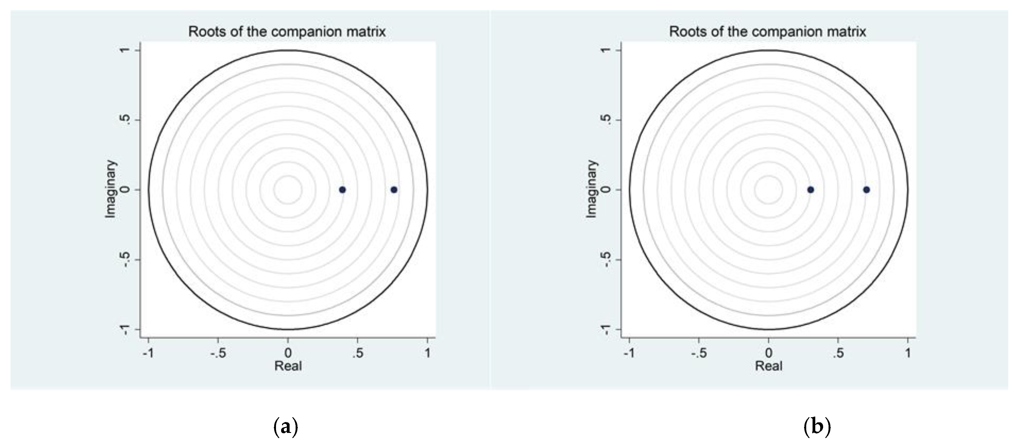
This research first checks the stability condition of the estimated PVAR through Impulse-Response Function. The resulting table and graph of eigenvalues confirm that all variables under this estimation are stable [53].
5.3. Results of PVAR and Corresponding FEVD
In order to utilize VAR estimation procedure into Panel data, restrictions needed to be added to ensure the underlying structure is in accordance with its cross-sectional part. In order to avoid the possible violation of this constraint in empirical analysis, there exists one reasonable solution to grant individual heterogeneity among target variables by employing fixed effect factors [48]. In this current research, Impulse Response Functions are adopted to estimate the impact of a certain variable’s shock on the present and future values of endogenous parameters while the null hypothesis will be suspended [70]. In order to overcome the shortage of auto-correlation, it is suggested to perform a shock Orthogonalization process to distinct similar components from residuals to each parameter through Cholesky decomposition methodology [9].
5.3.1. Results of PVAR
This section presents the results of PVAR model, Eigenvalue Stability Condition, Granger Causality Wald test, Forecast-Error Variance Decomposition (FEVD) and Impulse-response function. Table 7 shows the outcomes of PVAR model with one lag.
Here is the equation under estimation,
where is a six-variable vector (lnEF, lnGDP, lnFDI, lnEF_w, lnGDP_w, lnFDI_w), we use i to index countries in BRI project and t to index time (1990 to 2016), is the parameters and is white noise.
In order to facilitate the VAR model into panel data, it is suggested to impose restrictions, to ensure the underlying structures is in accordance with each cross-sectional unit, in our case, the different member countries of BRI project [48].
Table 11 demonstrate robustness under 1% level in general, which means strong robustness, especially, all variables display obvious correlation to itself, for example 0.811 for Total Ecological Footprint and 0.617 for FDI in model 1. Nonetheless, in model 2, Carbon Footprint exhibit positive self-correlation, which is in accordance with the case of Total Footprint. Even though both model 1 and model 2 illustrate significance in 1% level, their respective self-correlation is divergent among variables.
It is obvious from Table 11 that, response from changes of GDP to Ecological Footprint is sensitive, and a country with higher GDP is more likely to have higher Ecological Footprint which certifies the validity of Pollution Havens Hypothesis. While the cases for FDI are the same, response of Total Ecological Footprint is positively correlated with FDI, which imply Pollution Havens Hypothesis is true for these variables.
In detail, as for Carbon Footprint, similar tendency could also be observed: FDI, it exposed positive relationship with Ecological Footprint, which implies that higher total factor productivity and FDI evoke higher environmental risks in terms of ecological footprint.
The next step is to check the stability condition of PVAR model by adopting Eigenvalue Stability Condition. Table 12 demonstrates the graph and tables of eigenvalue stability condition. The Eigenvalue test indicated that the PVAR model is stable because all eigenvalues are inside of unity circle which can be observed in Table 13.
5.3.2. Results of the FEVD Estimates
Forecast-Error Variance Decomposition (from now on FEVD) was calculated through STATA command, based on a Cholesky decomposition of the residual covariance matrix of the underlying PVAR model. Standard errors and confidence intervals based on Monte Carlo estimation be calculated instead [71]. The analysis of nexus between ecological footprint, GDP, and FDI, complements the literature. The results of preliminary tests indicate the existence of low multi-collinearity, cross-section dependence, and unit roots.
Results of FEVD are displayed in Table 13. Due to the reason that standard errors are relatively large, the forecast error variance of Carbon Footprint is not obviously different from zero. Based on results of this test, it is possible to observe which variable exert stronger explaining power to our target variable: both FDI and Carbon Footprint explain better to their own changes, which are 63% and 99% respectively; as for the interactive influence, the explanatory power of Carbon Footprint to FDI is stronger than vice versa. These results demonstrate the fact that the bidirectional relationship between FDI and Carbon Footprint is not valid.
The variance decompositions display the significance of the total effect (Table 14). Development of Ecological Footprint was explained by the fluctuation of GDP and FDI. The result of the variance decomposition analysis for Ecological Footprint is demonstrated in Table 12, it is obvious that Total Ecological Footprint was negatively explained by GDP for 34% with robustness.
5.3.3. Impulse Response Functions
Through observing the outcome of Impulse Response Functions (from now on IRFs) estimation obtained from the PVAR estimation, it is possible to find how endogenous variables react to certain structural shocks over time. In this research, IRF outcomes are demonstrated in a 10-quarter period graph with 95% confident intervals. As it could be observed in Figure 1, the shaded area means a 95% confidence intermission.
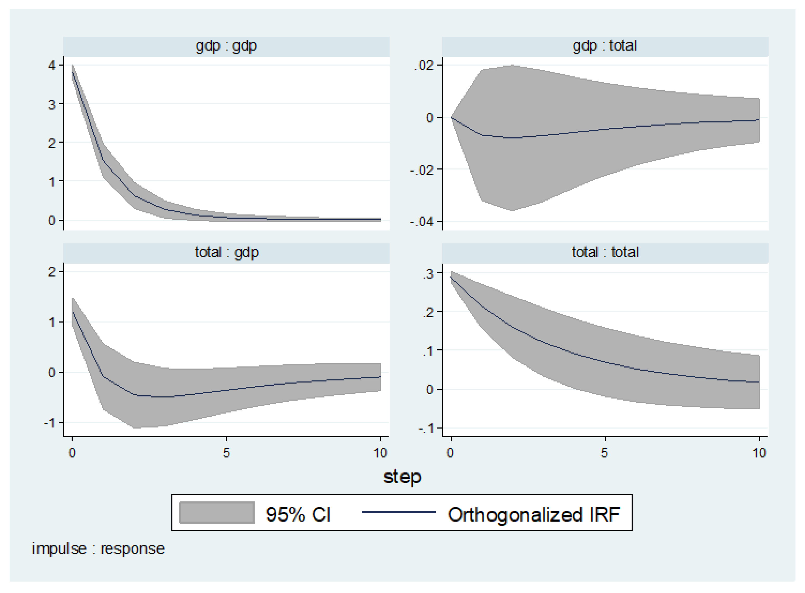
Figure 1 illustrated the structural IRFs of the endogenous variables to the shock of variables including themselves. IRF depicts the evolution of the variable Ecological Footprint, GDP, FDI along the time period 1990 to 2016, after a shock in a given point [72]. In this research, the first graph means response of FDI to FDI shock; confidence intervals are modulated using Gaussian estimation based on Monte Carlo collected from the estimated PVAR model. At the same time, Orthogonalized IRF are also estimated based on Cholesky decomposition [53]. Response of Ecological Footprint to FDI exposed a clear decreasing trend after a relatively stable period, which certifies the Pollution Halo Hypothesis: increasing trade and international investment deteriorate countries’ environment situations and makes poor countries into a pollution haven for their richer counterpart. The similar is true for the relationship between Ecological Footprint and GDP.
However, as for weight values, the outcome is more complicated than a simple one direction trend: it decreased at first and increased before further decline. When observing the Impulse Response Functions (IRFs) after accomplishing PVAR analysis, it is obvious to observe that endogenous variables response to certain structural shocks over the target time. Figure 1 illustrates the structural of the endogenous variables to the shocks of GDP, FDI respectively.
Based on results of this test displayed in Table 15, it is possible to observe which variable exert stronger explaining power to our target variable: Both FDI and Total Footprint explain better to their own changes, which are 64.4% and 84.2% respectively; as for the interactive influence, the explanatory power of Total Footprint to FDI is stronger than vice versa, the comparisons are 54.9% to 15.6%. These results demonstrate the fact that the bidirectional relationship between FDI and Total Footprint is not valid.
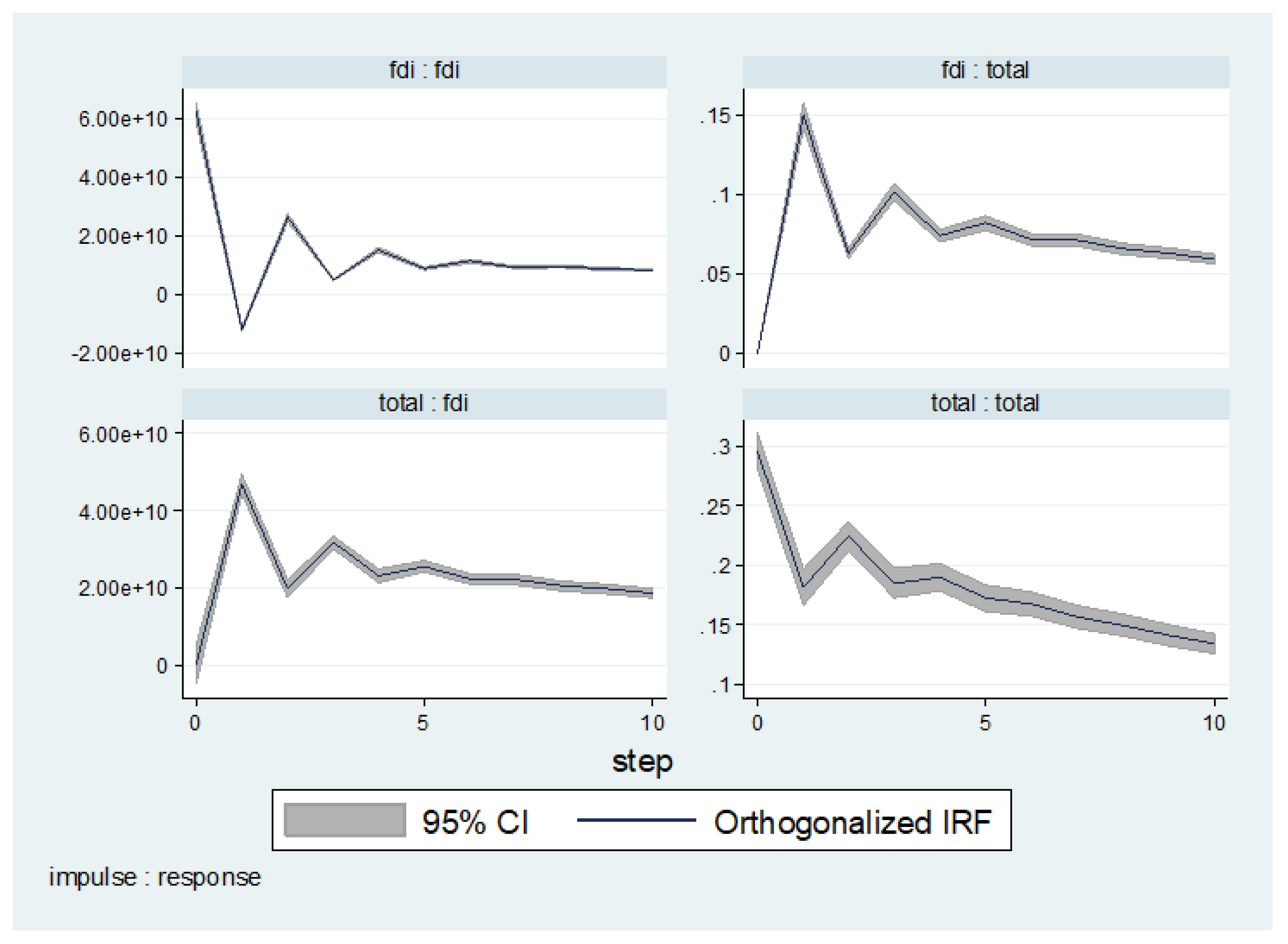
Figure 2 displays the structural IRF of a shock in FDI, GDP and Total Footprint on FDI, GDP and itself respectively. It indicates that, in this model a positive shock to FDI causes a steady increase. Although some of the impulse responses differ sharply, the response of FDI and Total demonstrates similar Footprint shock across the two orderings. FDI and Total Footprint display increasing trend in structural IRF test, which certifies Pollution Havens Hypothesis which is in opposite to Carbon Footprint.
The IRF results with GDP, FDI as well as with Ecological Footprint certify the dynamic correlation in line with the Pollution Havens Hypothesis we made in the beginning of this research. The empirical estimation displays that the interrelationship between Ecological Footprint and GDP, ecological footprint and FDI are robust among subsamples of Total Ecological Footprint and carbon ecological footprint.
Since FDI is of main interest in this research, a separate Impulse Response Function is performed to assistant detailed analysis and facilitates comparison. It is observed that, even though FDI and Total Footprint are comprised in both IRF test, there still exits great heterogeneity. In Figure 2, Total Footprint response to shocks of FDI positively, and the same is true when Total Footprint becomes the response variable. However, in Figure 3, the IRF correlation between FDI and Total Footprint demonstrates oscillation. Similar comparisons have been done to GDP and TFP, which could be observed in Appendix.
Overall, this investigation demonstrates that there exists a strong and robust causal relationship from FDI to Ecological Footprint and vice versa. Such conclusion can be made on GDP unidirectional relationship could be observe from Ecological Footprint to TFP. This result is in accordance with former research findings, where Tiwari certified unidirectional causality directed from energy consumption to GDP among Europe and Eurasian countries [73]. In this current research, further comparison between Carbon Footprint and Total Footprint sheds some intriguing phenomenon; in general, Total Footprint exhibits higher robustness and stronger correlations among variables.
To conclude, empirical outcomes of this study emphasize multiple essential policy significance to sustainable development in BRI member countries. First, due to the certification of FDI contribute to Pollution Havens Hypothesis in BRI countries, it is suggested for this initiative to pay more attention to the constitution of the FDI, when strive to economic development; balance between increasing the quantity of FDI and the possible pollution embedded in it. Second, this result is in consistent with increasing consciousness among countries in sustainable development trends, more stringent environmental policies are suggested to made to reduce ecological degradations; foreign investment should go through strict inspection before being approved. Lastly, most of BRI countries are developing ones or middle-income nations, it is recommended for these countries to reconsider their industry constitution, emphasize on renewable resource.
6. Conclusions
This research analyzed the environmental challenges on BRI project, with a special interest over FDI and interaction effect among its member countries. Current research is employed to examine the environmental issues embedded in BRI project, to be more specific: testify which of these three hypotheses (Pollution Havens Hypothesis, Pollution Halo Hypothesis, Environmental Kuznets Curve) is in accordance with the current development condition of BRI counties; whether there exists a bidirectional relationship among Ecological Footprint, Gross Domestic Production (GDP), FDI in BRI member countries. In this paper, Panel Vector Autoregression (PVAR) is utilized to analyze a dataset of 44-member countries in this initiative, ranges from 1990 to 2016, to empirically testify the environmental evaluation of this project. Results are analyzed on both long-run and short-run cases through Orthogonalized Impulse-Response Functions. Results of this research display a great heterogeneity among different target variables, FDI as a main variable of interest does expose a bidirectional relationship with Ecological Footprint, only Ecological Footprint demonstrates robust influence on FDI. In addition, Pollution Havens Hypothesis is true for FDI and GDP among BRI countries, after adopting weight values into PVAR estimation.
Further researches of this discipline are recommended to modify the measure of Ecological Footprint; make comparisons among country groups in different income levels. Besides, after adopting weight terms in existing PVAR model, heterogeneity between Carbon EF and Total EF in PVAR results disappears. In addition, by comparing results with and without weight terms, it is observed that, adding weight terms in PVAR model could increase convergence when performing IRF estimation. In accordance with most non-experimental analysis procedures, the current research is unable to provide confirmative evidence of causality. Further researches may fulfill this gap through more complexed methodologies such as instrumental variables, which could serve as an explanation of the causal nature embedded in the relationships we observed in current analysis. Apart from which, more detailed comparison between countries within BRI project and those who geographically connected but are not in the BRI group may exhibit consequential results.
Author Contributions
H.L. designed and analyzed econometric model, H.K. contributed to paper correction.
Funding
This work is sponsored by China Scholarship Council.
Acknowledgments
Special thanks are dedicated to Ohsang Kwon for his generous comments and inspiration. Besides, the authors are grateful to all committee members: Taeho Lee, Dongwhan An.
Conflicts of Interest
The authors declare no conflict of interest.
Appendix A. Results of Unit Root Test
Figure A1.
(a) Ecological footprint (Total), GDP, FDI, Total_w; (b) Ecological Footprint (Total) and FDI.
Figure A1.
(a) Ecological footprint (Total), GDP, FDI, Total_w; (b) Ecological Footprint (Total) and FDI.

Figure A2.
(a) Ecological footprint (Total), GDP; (b) Ecological Footprint (Total) and Total_w.

Figure A3.
(a) Ecological footprint (Carbon), GDP, FDI; (b) Carbon_w; Ecological Footprint (Carbon) and FDI.
Figure A3.
(a) Ecological footprint (Carbon), GDP, FDI; (b) Carbon_w; Ecological Footprint (Carbon) and FDI.

Figure A4.
(a) Ecological Footprint (Carbon) and GDP; (b) Ecological Footprint (Carbon) and Carbon-w.
Figure A4.
(a) Ecological Footprint (Carbon) and GDP; (b) Ecological Footprint (Carbon) and Carbon-w.

Figure A5.
(a) Unit root test comprises weight values (total); (b) Unit root test comprises weight value (carbon).
Figure A5.
(a) Unit root test comprises weight values (total); (b) Unit root test comprises weight value (carbon).

Appendix B. Results of the FEVD Estimates (Total Footprint)
Figure A6.
Ecological Footprint, GDP, FDI, TFP.

Figure A7.
Ecological Footprint and FDI.

Figure A8.
Ecological Footprint and GDP.

Appendix C. Results of the FEVD Estimates (Carbon Footprint)
Figure A9.
Ecological Footprint, GDP, FDI, TFP.

Figure A10.
Ecological Footprint and FDI.

Figure A11.
Ecological Footprint and GDP.

Appendix D. Results of the FEVD Estimates (Forecast-Error Variance Decomposition)

Table A1.
FEVD results response from Total Ecological Footprint to other variables.
| Total | GDP | FDI | Total_w | GDP_w | FDI_w | ||
|---|---|---|---|---|---|---|---|
| Total | 0 | 0 | 0 | 0 | 0 | 0 | 0 |
| 1 | 1 | 0 | 0 | 0 | 0 | 0 | |
| 2 | 0.2729872 | 0.3113742 | 0.1904543 | 0.0559764 | 0.1024007 | 0.0162377 | |
| 3 | 0.1042024 | 0.2590105 | 0.0746439 | 0.0754784 | 0.0620527 | 0.0074815 | |
| 4 | 0.0503231 | 0.2311534 | 0.0345107 | 0.0573566 | 0.0547333 | 0.0085252 | |
| 5 | 0.0507172 | 0.2302332 | 0.0269293 | 0.0455589 | 0.0501147 | 0.0080496 | |
| 6 | 0.0524706 | 0.2224286 | 0.0231806 | 0.0434394 | 0.0462321 | 0.0072384 | |
| 7 | 0.0538884 | 0.2199838 | 0.022402 | 0.0428509 | 0.0450956 | 0.0070641 | |
| 8 | 0.0544239 | 0.2191629 | 0.0221126 | 0.0425863 | 0.044692 | 0.0069989 | |
| 9 | 0.0546112 | 0.2188358 | 0.0220114 | 0.0425053 | 0.044547 | 0.0069752 | |
| 10 | 0.054685 | 0.2187308 | 0.021981 | 0.0424776 | 0.0444977 | 0.0069675 | |
Table A2.
FEVD results response from GDP to other variables.
| Total | GDP | FDI | Total_w | GDP_w | FDI_w | ||
|---|---|---|---|---|---|---|---|
| GDP | 0 | 0 | 0 | 0 | 0 | 0 | 0 |
| 1 | 0.5803802 | 0.4196198 | 0 | 0 | 0 | 0 | |
| 2 | 0.2960931 | 0.4130535 | 0.1940907 | 0.0100347 | 0.0466805 | 0.0114994 | |
| 3 | 0.2056349 | 0.2879183 | 0.1873958 | 0.015766 | 0.0411985 | 0.0167622 | |
| 4 | 0.1364163 | 0.2440374 | 0.1135423 | 0.03444 | 0.0491563 | 0.0159092 | |
| 5 | 0.0764843 | 0.2368277 | 0.0427532 | 0.0354312 | 0.04693 | 0.0092217 | |
| 6 | 0.0574348 | 0.216825 | 0.0237428 | 0.0414286 | 0.0434009 | 0.0069177 | |
| 7 | 0.0557434 | 0.2185673 | 0.0225232 | 0.0423138 | 0.0443466 | 0.007009 | |
| 8 | 0.0549465 | 0.2185257 | 0.0219544 | 0.0423719 | 0.0443564 | 0.0069473 | |
| 9 | 0.0547751 | 0.2185597 | 0.0219416 | 0.0424481 | 0.0444277 | 0.0069567 | |
| 10 | 0.0547484 | 0.2186496 | 0.02196 | 0.0424557 | 0.0444587 | 0.0069618 | |
Table A3.
FEVD results response from FDI to other variables.
| Total | GDP | FDI | Total_w | GDP_w | FDI_w | ||
|---|---|---|---|---|---|---|---|
| FDI | 0 | 0 | 0 | 0 | 0 | 0 | 0 |
| 1 | 0.3923546 | 0.4005113 | 0.0907443 | 0 | 0 | 0 | |
| 2 | 0.215026 | 0.3464602 | 0.2273232 | 0.0010855 | 0.0634985 | 0.0277523 | |
| 3 | 0.228313 | 0.3308179 | 0.2334994 | 0.0010356 | 0.0635267 | 0.0310513 | |
| 4 | 0.2274611 | 0.3214023 | 0.2249864 | 0.0034546 | 0.0609543 | 0.0299885 | |
| 5 | 0.2222104 | 0.3144613 | 0.222342 | 0.0034222 | 0.0608899 | 0.0296872 | |
| 6 | 0.2236479 | 0.3055883 | 0.2098522 | 0.0038 | 0.0581065 | 0.0282042 | |
| 7 | 0.1989613 | 0.2761485 | 0.1723641 | 0.0071741 | 0.0502627 | 0.0233663 | |
| 8 | 0.13535 | 0.2343416 | 0.0949496 | 0.0223688 | 0.0425361 | 0.0145486 | |
| 9 | 0.0791403 | 0.2175597 | 0.0381161 | 0.035672 | 0.0413326 | 0.0083966 | |
| 10 | 0.0603904 | 0.2154625 | 0.023771 | 0.0407164 | 0.0426275 | 0.0069747 | |
Table A4.
FEVD results response from Total Ecological Footprint weight to other variables.
| Total | GDP | FDI | Total_w | GDP_w | FDI_w | ||
|---|---|---|---|---|---|---|---|
| Total_w | 0 | 0 | 0 | 0 | 0 | 0 | 0 |
| 1 | 0.5798764 | 0.2451898 | 0.0697621 | 0.073704 | 0 | 0 | |
| 2 | 0.3227322 | 0.2936386 | 0.2428648 | 0.0327497 | 0.04847 | 0.0150644 | |
| 3 | 0.2840617 | 0.2900498 | 0.2588234 | 0.0275094 | 0.0718941 | 0.0292734 | |
| 4 | 0.2236199 | 0.2875167 | 0.1884545 | 0.0238179 | 0.060882 | 0.0214839 | |
| 5 | 0.1288141 | 0.2211411 | 0.0919521 | 0.0395862 | 0.0441483 | 0.0117798 | |
| 6 | 0.0746816 | 0.2223146 | 0.0387449 | 0.0416383 | 0.0450886 | 0.0084859 | |
| 7 | 0.0580627 | 0.2179335 | 0.0238557 | 0.0418764 | 0.0438804 | 0.0070334 | |
| 8 | 0.0553997 | 0.2180903 | 0.022205 | 0.0423937 | 0.0442652 | 0.0069637 | |
| 9 | 0.0549365 | 0.2185673 | 0.0219966 | 0.0424195 | 0.0444026 | 0.0069593 | |
| 10 | 0.0547727 | 0.2185882 | 0.021945 | 0.0424516 | 0.0444327 | 0.0069569 | |
Table A5.
FEVD results response from GDP_w to other variables.
| Total | GDP | FDI | Total_w | GDP_w | FDI_w | ||
|---|---|---|---|---|---|---|---|
| GDP_w | 0 | 0 | 0 | 0 | 0 | 0 | 0 |
| 1 | 0.0587837 | 0.2363376 | 0.0164409 | 0.0437329 | 0.2316438 | 0 | |
| 2 | 0.1780399 | 0.2084704 | 0.0813591 | 0.1251542 | 0.0650408 | 0.0002897 | |
| 3 | 0.0923775 | 0.1580604 | 0.0271952 | 0.0768084 | 0.0306546 | 0.0005893 | |
| 4 | 0.0607027 | 0.1992721 | 0.0228974 | 0.0493401 | 0.0435409 | 0.0069037 | |
| 5 | 0.0573754 | 0.2201142 | 0.0234538 | 0.0421934 | 0.0452801 | 0.0072447 | |
| 6 | 0.0550688 | 0.2177749 | 0.0217253 | 0.0424681 | 0.0441055 | 0.0068639 | |
| 7 | 0.0549094 | 0.2183572 | 0.0219344 | 0.042514 | 0.0443592 | 0.0069464 | |
| 8 | 0.0547901 | 0.2185965 | 0.0219449 | 0.0424563 | 0.0444316 | 0.0069574 | |
| 9 | 0.0547411 | 0.2186307 | 0.021952 | 0.0424608 | 0.044454 | 0.0069603 | |
| 10 | 0.0547322 | 0.2186589 | 0.0219605 | 0.0424621 | 0.0444647 | 0.0069623 | |
Table A6.
FEVD results response from FDI_w to other variables.
| Total | GDP | FDI | Total_w | GDP_w | FDI_w | ||
|---|---|---|---|---|---|---|---|
| GDP_w | 0 | 0 | 0 | 0 | 0 | 0 | 0 |
| 1 | 0.0017691 | 0.3957767 | 0.0325533 | 0.0178445 | 0.1265757 | 0.011514 | |
| 2 | 0.0466656 | 0.2538268 | 0.0307276 | 0.0455623 | 0.0565016 | 0.0053304 | |
| 3 | 0.054623 | 0.2236274 | 0.0221681 | 0.043589 | 0.0445038 | 0.0061264 | |
| 4 | 0.0532808 | 0.2186349 | 0.0214142 | 0.0421125 | 0.0448085 | 0.0069024 | |
| 5 | 0.0543636 | 0.2197206 | 0.0222199 | 0.0421252 | 0.0449794 | 0.0070586 | |
| 6 | 0.0545773 | 0.2190187 | 0.0220189 | 0.0423565 | 0.0446001 | 0.0069782 | |
| 7 | 0.0546678 | 0.2187463 | 0.0219771 | 0.0424497 | 0.0445048 | 0.0069665 | |
| 8 | 0.0547073 | 0.2187033 | 0.0219708 | 0.0424597 | 0.0444839 | 0.0069651 | |
| 9 | 0.0547176 | 0.2186799 | 0.0219649 | 0.0424624 | 0.0444741 | 0.0069636 | |
| 10 | 0.0547222 | 0.2186726 | 0.0219636 | 0.0424633 | 0.0444709 | 0.0069631 | |
References
- Yu, H. Motivation behind China’s ‘One Belt, One Road’ initiatives and establishment of the Asian infrastructure investment bank. J. Contemp. China 2017, 26, 353–368. [Google Scholar] [CrossRef]
- Tracy, E.F.; Shvarts, E.; Simonov, E.; Babenko, M. China’s new Eurasian ambitions: The environmental risks of the Silk Road Economic Belt. Eurasian Geogr. Econ. 2017, 58, 56–88. [Google Scholar] [CrossRef]
- Hu, J.; Wang, Z.; Lian, Y.H.; Huang, Q.H. Environmental regulation, foreign direct investment and green technological progress—Evidence from Chinese manufacturing industries. Int. J. Environ. Res. Public Health 2018, 15, 221. [Google Scholar] [CrossRef]
- Levi, M. Go east, young oilman. Foreign Aff. 2015, 94, 108–117. [Google Scholar]
- Harashima, Y.; Morita, T. A comparative study on environmental policy development processes in the three East Asian countries: Japan, Korea, and China. Environ. Econ. Policy Stud. 1998, 1, 39–67. [Google Scholar] [CrossRef]
- Stroik, P.C. Technology, Trade and the Environment. Ph.D. Thesis, University of California, Irvine, CA, USA, 2016. [Google Scholar]
- Doytch, N. FDI halo vs. pollution haven hypothesis. In Proceedings of the New York State Economics Association, New York, NY, USA, 5–6 October 2012. [Google Scholar]
- Doytch, N.; Uctum, M. Globalization and the Environmental Spillovers of Sectoral FDI. Available online: http://www.freit.org/WorkingPapers/Papers/ForeignInvestment/FREIT530.pdf (accessed on 14 September 2018).
- Sassi, S.; Gasmi, A. The dynamic relationship between corruption-inflation: Evidence from panel vector autoregression. Jpn. Econ. Rev. 2017, 68, 458–469. [Google Scholar] [CrossRef]
- Canova, F.; Ciccarelli, M. Panel Vector Autoregressive Models: A Survey, 1st ed.; Emerald Group Publishing Limited: Bingley, UK, 2013; pp. 205–246. [Google Scholar]
- Zhang, N.; Liu, Z.; Zheng, X.M.; Xue, J.J. Carbon footprint of China’s belt and road. Science 2017, 357, 1107. [Google Scholar] [CrossRef] [PubMed]
- Wang, C.J.; Wang, F. China can lead on climate change. Science 2017, 357, 764. [Google Scholar] [CrossRef] [PubMed]
- Zwerg, A.M.; Carlos, L.; Vieira, A. The impact of foreign direct investment on developing economies and the environment. AD-minister 2008, 8, 111–128. [Google Scholar]
- He, J. Pollution haven hypothesis and environmental impacts of foreign direct investment: The case of industrial emission of sulfur dioxide (SO2) in Chinese provinces. Ecol. Econ. 2006, 60, 228–245. [Google Scholar] [CrossRef]
- Jiang, Y.Q. Foreign direct investment, pollution, and the environmental quality: A model with empirical evidence from the Chinese regions. Int. Trade J. 2015, 29, 212–227. [Google Scholar] [CrossRef]
- Driffield, N.; Taylor, K. FDI and the labour market: A review of the evidence and policy implications. Oxf. Rev. Econ. Pol. 2000, 16, 90–103. [Google Scholar] [CrossRef]
- Cole, M.A. Trade, the pollution haven hypothesis and the environmental Kuznets curve: Examining the linkages. Ecol. Econ. 2004, 48, 71–81. [Google Scholar] [CrossRef]
- Birdsall, N.; Wheeler, D. Trade policy and industrial pollution in Latin America: Where are the pollution havens? J. Environ. Dev. 1993, 2, 137–149. [Google Scholar] [CrossRef]
- Mabey, N.; McNally, R. Foreign Direct Investment and the Environment: From Pollution Havens to Sustainable Development. Available online: http://www.oecd.org/investment/mne/2089912.pdf (accessed on 14 September 2018).
- Brucal, A.; Javorcik, B.; Love, I. Pollution Havens or Halos? Evidence from Foreign Acquisitions in Indonesia. Available online: https://editorialexpress.com/cgi-bin/conference/download.cgi?db_name=SED2017&paper_id=306 (accessed on 14 September 2018).
- Grossman, G.M.; Krueger, A.B. The inverted-U: What does it mean? Env. Dev. Econ. 2008, 1, 119–122. [Google Scholar] [CrossRef]
- Stern, D.I. The environmental Kuznets curve after 25 years. J. Bioecon. 2017, 19, 7–28. [Google Scholar] [CrossRef]
- Pao, H.T.; Tsai, C.M. Multivariate Granger causality between CO2 emissions, energy consumption, FDI (foreign direct investment) and GDP (gross domestic product): Evidence from a panel of BRIC (Brazil, Russian Federation, India, and China) countries. Energy 2011, 36, 685–693. [Google Scholar] [CrossRef]
- Girma, S. Absorptive capacity and productivity spillovers from FDI: A threshold regression analysis. Oxf. Bull. Econ. Stat. 2005, 67, 281–306. [Google Scholar] [CrossRef]
- Moran, T.H. Does Foreign Direct Investment Promote Development, 3rd ed.; Institute for International Economics: Washington, DC, USA, 2005; pp. 281–313. [Google Scholar]
- Wei, Y.; Liu, X. Productivity spillovers from R&D, exports and FDI in China’s manufacturing sector. J. Int. Bus. Stud. 2006, 37, 544–557. [Google Scholar] [CrossRef]
- Holtz-Eakin, D.; Newey, W.; Rosen, H.S. Estimating vector autoregressions with panel data. Econometrica 1988, 6, 1371–1395. [Google Scholar] [CrossRef]
- Brana, S.; Djigbenou, M.L.; Prat, S. Global excess liquidity and asset prices in emerging countries: A PVAR approach. Emerg. Mark. Rev. 2012, 13, 256–267. [Google Scholar] [CrossRef]
- Canova, F.; Ciccarelli, M. Estimating multicountry VAR models. Int. Econ. Rev. 2009, 50, 929–959. [Google Scholar] [CrossRef]
- Ang, A.; Piazzesi, M. A no-arbitrage vector autoregression of term structure dynamics with macroeconomic and latent variables. J. Monetary Econ. 2003, 50, 745–787. [Google Scholar] [CrossRef] [Green Version]
- Enders, W.; Sandler, T. The effectiveness of antiterrorism policies: A vector-autoregression-intervention analysis. Am. Political Sci. Rev. 1993, 87, 829–844. [Google Scholar] [CrossRef]
- Toda, H.Y.; Phillips, P.C. Vector autoregression and causality: A theoretical overview and simulation study. Econ. Rev. 1994, 13, 259–285. [Google Scholar] [CrossRef]
- Canh, N.T.; Phong, N.A. Effect of public investment on private investment and economic growth: Evidence from Vietnam by economic industries. Appl. Econ. Financ. 2018, 5, 95–110. [Google Scholar] [CrossRef]
- Koengkan, M. The nexus between energy consumption, economic growth, and urbanization in Latin American and Caribbean countries: An approach with PVAR model. Rev. Valore 2017, 2, 202–219. [Google Scholar] [CrossRef] [Green Version]
- Ramadhani, N.Q.; Saraswati, E.; Fuad, A. Social responsibility and value added acreation. IJournals 2017, 6, 1–9. [Google Scholar]
- Javorcik, B.S. Does foreign direct investment increase the productivity of domestic firms? In search of spillovers through backward linkages. Am. Econ. Rev. 2004, 94, 605–627. [Google Scholar] [CrossRef]
- Qu, J.Z.; Zhang, Z.M. Relationship between Financial Development and International Trade in China—Based on the Data of 1991–2005. J. Int. Trade 2008, 1, 16. [Google Scholar]
- Yang, W.P.; Yuan, X.L. The Effect of Foreign Trade and FDI on Environmental Pollution: An analysis based on the Impulse Response Function of Time Series in China: 1982–2006. World Econ. Stud. 2008, 12, 12. [Google Scholar]
- Arellano, M.; Bover, O. Another look at the instrumental variable estimation of error-components models. J. Econ. 1995, 68, 29–51. [Google Scholar] [CrossRef]
- Baltagi, B. Econometric Analysis of Panel Data, 4th ed.; Instituto de Economía, INTA: Buenos Aires, Argentina, 2008. [Google Scholar]
- Kneller, R.; Pisu, M. Industrial link ages and export spillovers from FDI. World Econ. 2007, 30, 105–134. [Google Scholar] [CrossRef]
- Dong, B.; Gong, J.; Zhao, X. FDI and environmental regulation: Pollution haven or a race to the top? J. Reg. Econ. 2012, 41, 216–237. [Google Scholar] [CrossRef]
- Lairson, T.D. The Global Strategic Environment of the BRI: Deep Interdependence and Structural Power, in China’s Belt and Road Initiative, 1st ed.; Palgrave Macmillan: Cham, Switzerland, 2018; pp. 35–53. [Google Scholar]
- Neequaye, N.A.; Oladi, R. Environment, growth, and FDI revisited. Int. Rev. Econ. Financ. 2015, 39, 47–56. [Google Scholar] [CrossRef]
- Dovern, J.; Meier, C.P.; Vilsmeier, J. How resilient is the German banking system to macroeconomic shocks? J. Bank Financ. 2010, 34, 1839–1848. [Google Scholar] [CrossRef] [Green Version]
- Dees, S.; Mauro, F.; Pesaran, M.H.; Smith, L.V. Exploring the international linkages of the euro area: A global VAR analysis. J. Appl. Econ. 2007, 22, 1–38. [Google Scholar] [CrossRef]
- Lof, M.; Malinen, T. Does sovereign debt weaken economic growth? A panel VAR analysis. Econ. Lett. 2014, 122, 403–407. [Google Scholar] [CrossRef] [Green Version]
- Love, I.; Zicchino, L. Financial development and dynamic investment behavior: Evidence from panel VAR. Quart. Rev. Econ. Financ. 2006, 46, 190–210. [Google Scholar] [CrossRef] [Green Version]
- Metiu, N.; Hilberg, B.; Grill, M. Financial Shocks, Credit Regimes, and Global Spillovers. Available online: https://www.bundesbank.de/Redaktion/EN/Downloads/Publications/Discussion_Paper_1/2015/2015_03_17_dkp_04.pdf?__blob=publicationFile (accessed on 14 September 2018).
- Sadorsky, P. The impact of financial development on energy consumption in emerging economies. Energy Policy 2010, 38, 2528–2535. [Google Scholar] [CrossRef]
- Raddatz, C. Are external shocks responsible for the instability of output in low-income countries? J. Dev. Econ. 2007, 84, 155–187. [Google Scholar] [CrossRef]
- Li, Q.; Hu, H.; Luo, H.J.; Lin, L.Y.; Shi, Y.; Zhang, Y.J.; Zhou, L. Two-way coupling relationship between economic growth and environmental pollution-Regional difference analysis based on PVAR model. Acta Scientiae Circumstantiae 2015, 6, 1875–1886. [Google Scholar]
- Abrigo, M.R.; Love, I. Estimation of Panel Vector Autoregression in Stata: A Package of Programs. Available online: http://paneldataconference2015.ceu.hu/Program/Michael-Abrigo.pdf (accessed on 14 September 2018).
- Kuzyk, L.W. The ecological footprint housing component: A geographic information system analysis. Ecol. Indic. 2012, 16, 31–39. [Google Scholar] [CrossRef]
- Świąder, M.; Szewrański, S.; Kazak, J.K.; Hoof, J.V.; Lin, D.; Wackernagel, M.; Alves, A. Application of ecological footprint accounting as a part of an integrated assessment of environmental carrying capacity: A case study of the footprint of food of a large city. Resources 2018, 7, 52. [Google Scholar] [CrossRef]
- Borucke, M.; Moore, D.; Cranston, G.; Gracey, K.; Iha, K.; Larson, J.; Lazarus, E.; Morales, J.C.; Wackernagel, M.; Galli, A. Accounting for demand and supply of the biosphere’s regenerative capacity: The National Footprint Accounts’ underlying methodology and framework. Ecol. Indic. 2013, 24, 518–533. [Google Scholar] [CrossRef]
- Monfreda, C.M.; Wackernagel, M.; Deumling, D. Establishing national natural capital accounts based on detailed ecological footprint and biological capacity assessments. Land Use Policy 2004, 21, 231–246. [Google Scholar] [CrossRef]
- Bank, T.W. World Development Indicators 2014. 2014. Available online: https://books.google.com.hk/books?hl=zh-TW&lr=&id=pQqKAwAAQBAJ&oi=fnd&pg=PP1&dq=World+Development+Indicators+2014&ots=UPXPhnMR4D&sig=VMnHpQLEA69eghugijTXQTJBcP4&redir_esc=y#v=onepage&q=World%20Development%20Indicators%202014&f=false (accessed on 25 September 2018).[Green Version]
- Doytch, N.; Narayan, S. Does FDI influence renewable energy consumption? An analysis of sectoral FDI impact on renewable and non-renewable industrial energy consumption. Energy Econ. 2016, 54, 291–301. [Google Scholar] [CrossRef]
- Engle, R.F.; Granger, C.W. Co-integration and error correction: Representation, estimation, and testing. Econometrica 1987, 2, 251–276. [Google Scholar] [CrossRef]
- Friedl, B.; Getzner, M. Determinants of CO2 emissions in a small open economy. Ecol. Econ. 2003, 45, 133–148. [Google Scholar] [CrossRef]
- Elliot, B.; Rothenberg, T.; Stock, J. Efficient tests of the unit root hypothesis. Econometrica 1996, 64, 13–36. [Google Scholar]
- Akaike, H. Fitting autoregressive models for prediction. Ann. Inst. Stat. Math. 1969, 1, 243–247. [Google Scholar] [CrossRef]
- Hannan, E.J.; Quinn, B.G. The determination of the order of an autoregression. J. R. Stat. Soc. 1979, 2, 190–195. [Google Scholar]
- Schwarz, G. Estimating the dimension of a model. Ann. Stat. 1978, 2, 461–464. [Google Scholar] [CrossRef]
- Lütkepohl, H. New Introduction to Multiple Time Series Analysis, 1st ed.; Springer Science & Business Media: Berlin, Germany, 2005. [Google Scholar]
- Asafu-Adjaye, J. The relationship between energy consumption, energy prices and economic growth: Time series evidence from Asian developing countries. Energy Econ. 2000, 22, 615–625. [Google Scholar] [CrossRef]
- Sigmund, M.; Ferstl, R.; Unterkofler, D. Panel Vector Autoregression in R with the Package Panelvar. Available online: https://papers.ssrn.com/sol3/Delivery.cfm/SSRN_ID3194239_code1405094.pdf?abstractid=2896087&mirid=1 (accessed on 14 September 2018).
- Becketti, S. Introduction to Time Series Using Stata, 1st ed.; Stata Press: College Station, TX, USA, 2013. [Google Scholar]
- Henriques, I.; Sadorsky, P. Oil prices and the stock prices of alternative energy companies. Energy Econ. 2008, 30, 998–1010. [Google Scholar] [CrossRef]
- Winkler, A.M.; Ridgway, G.R.; Webster, M.A.; Smith, S.M.; Nichols, T.E. Permutation inference for the general linear model. Neuroimage 2014, 92, 381–397. [Google Scholar] [CrossRef] [PubMed]
- Pesaran, H.H.; Shin, Y.C. Generalized impulse response analysis in linear multivariate models. Econ. Lett. 1998, 58, 17–29. [Google Scholar] [CrossRef] [Green Version]
- Tiwari, A.K. Comparative performance of renewable and nonrenewable energy source on economic growth and CO2 emissions of Europe and Eurasian countries: A PVAR approach. Econ. Bull. 2011, 31, 2356–2372. [Google Scholar]
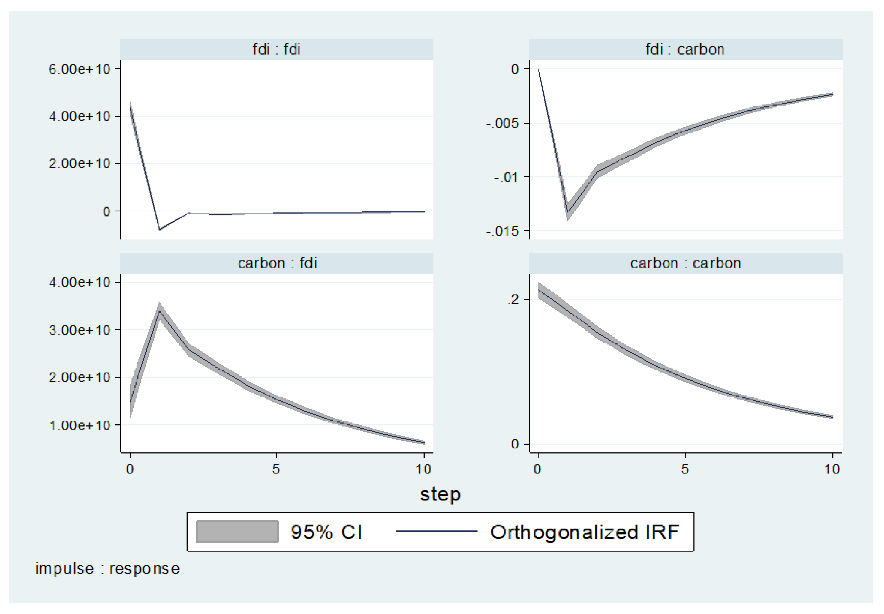
Figure 1.
Impulse Response Functions (IRFs) Results of Ecological Footprint (Carbon), GDP, and FDI.

Figure 2.
Results of ecological footprint (Total), GDP, FDI.

Figure 3.
Results of ecological footprint (Total), FDI.

Table 1.
Three major hypotheses on FDI’s environmental spillover effect.
| Name of the Hypothesis | Meaning | Literature |
|---|---|---|
| Pollution Havens Hypothesis (PHH) | Local government tend to make lax environmental standards in order attract more FDI and obtain relative advantages in regional economic development | [3] [17] [18] |
| FDI Halo Hypothesis | FDI is hypothesized to exert positive environmental spillover effects, because FDI is supposed to be able to transfer advance technologies from developed countries to under-developed ones. | [7] [19] [20] |
| EKC Hypothesis | Economic development influences environment through scale, composition and technique effect which leads to an inverted U-shaped relationship between the two variables. | [21] [22] |
Table 2.
Literature summary concerning Foreign Direct Investment (FDI) and environment.
| Author | Dependent Variable | Independent Variable | Region | Time | Method |
|---|---|---|---|---|---|
| Hoffmann et al., 2005 | CO2, SO2 Emission | FDI | 112 countries | 1990–2005 | Granger causality analysis |
| Girma, 2005 | Changes in TFP | FDI, absorptive capacity (ABC) | UK | 1989–1999 | Endogenous threshold model, input Cobb–Douglas |
| Wei and Liu, 2006 | TFP | R&D, export, FDI spillover | China | 1998–2001 | Cobb–Douglas production function |
| Zheng et al., 2010 | Housing Price | Productivity, geography, quality of life | 35 major Chinese cities | 1991–2006 | Hedonic regression |
| Bekhet and bt Othman, 2011 | Electricity Consumption | CPI, GDP and FDI | Malaysia | 1971–2009 | VECM |
| Pao and Tsai, 2011 | CO2 Emissions | Energy consumption, FDI, Economic Growth | BRIC | 1980–2005 | Panel cointegration |
| Jiang, 2015 | Pollution emission | FDI, output, capital stock, human capital stock, labor input | China, 28 provincial-level | 1997–2012 | OLS, Panel data |
| Doytch and Narayan, 2016 | Energy consumption | GDP, FDI, net FDI capital inflow share of GDP | 74 Countries | 1985–2012 | Dynamic panel estimation |
Table 3.
Demonstration and comparison among different types Vector Autoregression (VAR) models.
| VAR Types | Characteristics |
|---|---|
| VAR |
|
| SVAR (Structural VAR) |
|
| GVAR (Global VAR) |
|
| PVAR (Panel VAR) |
|
| TVAR (Threshold VAR) |
|
Table 4.
Panel Vector Autoregression (PVAR) model applications in former literature.
| PVAR applications | Energy consumption, financial development, economic growth [50] |
| Financial development, investment decisions [48] | |
| Corruption and inflation [9] | |
| External shocks (commodity price, natural disaster, international economy) to output instability [51] | |
| The influence of global excess liquidity on commodities and asset prices [28] | |
| Two-dimension analysis between economic growth and pollution [52] |
Table 5.
A summary of dataset.
| Variables | Observations | Mean | Standard Deviation | Minimum | Maximum |
|---|---|---|---|---|---|
| Ecological Footprint (Carbon) | 1017 | 1.6899 | 1.284045 | 0.021174 | 6.704063 |
| Ecological Footprint (Total) | 1017 | 3.0032 | 1.821681 | 0.4308162 | 9.314663 |
| GDP | 1538 | 3.1564 | 8.1022 | −99.2 | 60.3 |
| FDI | 1030 | 7.13 × 10 9 | 2.45 × 10 10 | −2.09 × 10 10 | 2.91 × 10 11 |
Table 6.
Results of unit root test.
| Variables | Inverse Chi-Squared | Inverse Normal | Inverse Logit | Modified Inverse Chi-Squared |
|---|---|---|---|---|
| 268.94 (0.00) | –9.87 (0.00) | –10.42 (0.00) | 13.64 (0.00) | |
| 273.16 (0.00) | –10.05 (0.00) | –10.68 (0.00) | 13.96 (0.00) | |
| 725.05 (0.00) | –21.04 (0.00) | –26.46 (0.00) | 40.47 (0.00) | |
| 156.98 (0.00) | –6.13 (0.00) | –5.89 (0.00) | 6.09 (0.00) | |
| 486.11 (0.00) | –13.96 (0.00) | –17.27 (0.00) | 24.64 (0.00) | |
| 488.03 (0.00) | –14.26 (0.00) | –17.41 (0.00) | 24.77 (0.00) | |
| 725.05 (0.00) | –21.03 (0.00) | –26.45 (0.00) | 40.46 (0.00) | |
| 302.32 (0.00) | –9.35 (0.00) | –10.31 (0.00) | 12.47 (0.00) |
Values in parentheses are p-values.
Table 7.
Lag selection outcome between Ecological Footprint and GDP.
| Lag | Interactions between EF (Carbon) and GDP | Interactions between EF (Total) and GDP | ||||||||
|---|---|---|---|---|---|---|---|---|---|---|
| CD | J | MBIC | MAIC | MQIC | CD | J | MBIC | MAIC | MQIC | |
| 1 | 0.99 | 11.5 | −68.7 | −12.5 | −34.1 | 0.99 | 15.2 | −65.0 | −8.8 | −30.4 |
| 2 | 0.99 | 7.0 | −46.4 | −8.9 | −23.4 | 0.99 | 8.6 | −44.8 | −7.4 | −21.8 |
| 3 | 0.99 | 3.3 | −23.5 | −4.7 | −11.9 | 0.99 | 4.6 | −22.2 | −3.5 | −10.6 |
Table 8.
Lag selection outcome between Ecological Footprint and FDI.
| Lag | Interactions between EF (Carbon) and FDI | Interactions between EF (Total) and FDI | ||||||||
|---|---|---|---|---|---|---|---|---|---|---|
| CD | J | MBIC | MAIC | MQIC | CD | J | MBIC | MAIC | MQIC | |
| 1 | 0.99 | 11.82 | −68.3 | −12.18 | −33.76 | 0.992 | 13.26 | −66.9 | −10.74 | −32.32 |
| 2 | 0.99 | 6.98 | –46.4 | −9.02 | −23.41 | 0.993 | 6.33 | −47.1 | −9.67 | −24.05 |
| 3 | 0.98 | 3.67 | −23.0 | −4.33 | −11.52 | 0.984 | 1.08 | −25.6 | −6.92 | −14.11 |
Table 9.
Lag selection outcome between Ecological Footprint_w and GDP_w.
| Lag | Interactions between EF_w(carbon)and GDP | Interactions between EF_w(total) and GDP | ||||||||
|---|---|---|---|---|---|---|---|---|---|---|
| CD | J | MBIC | MAIC | MQIC | CD | J | MBIC | MAIC | MQIC | |
| 1 | 0.99 | 18.18 | −61.98 | −5.23 | −27.40 | 0.99 | 0.18 | −63.88 | −7.73 | −29.31 |
| 2 | 0.99 | 10.99 | −42.45 | −5.01 | −19.39 | 0.97 | 0.28 | −43.58 | −6.14 | −20.53 |
| 3 | −1.52 | 3.34 | −23.38 | −4.66 | −11.86 | −9.49 | 0.33 | −22.11 | −3.39 | −10.58 |
Table 10.
Lag selection outcome between Ecological Footprint_w and FDI_w.
| Lag | Interactions between EF_w(carbon) and FDI | Interactions between EF_w(total) and FDI_w | ||||||||
|---|---|---|---|---|---|---|---|---|---|---|
| CD | J | MBIC | MAIC | MQIC | CD | J | MBIC | MAIC | MQIC | |
| 1 | 0.999 | 15.02 | –63.79 | –8.98 | –30.15 | 0.999 | 16.41 | –62.40 | –7.59 | –28.76 |
| 2 | 0.999 | 11.73 | –40.82 | –4.27 | –18.39 | 0.999 | 5.73 | –46.82 | –10.27 | –24.39 |
| 3 | 0.978 | 6.86 | –19.41 | –1.34 | –8.19 | 0.974 | 8.93 | –17.35 | 0.93 | –6.13 |
Table 11.
Result of PVAR.
| Response of | Response to | |||||
|---|---|---|---|---|---|---|
| D (Ln_EF) | D (Ln_GDP) | D (Ln_FDI) | D (Ln_EFw) | D (Ln_GDPw) | D (Ln_FDIw) | |
| Mode1. Ecological Footprint (Total) and GDP, FDI, and their weights | ||||||
| D (Ln_EF) | 8.10 × 10⁻¹ (1.57 × 10⁹) | 6.10× 10⁻¹ (8.28 × 10⁸) | 3.46 × 10⁻¹² (1.01 × 10⁹) | −2.64 (−2.64 × 10⁹) | −1.41 × 10⁻² (−1.95 × 10⁸) | 4.94 × 10⁻¹¹ (2.12 × 10⁹) |
| D (Ln_GDP) | 3.58 (6.94 × 10⁹) | 6.80 × 10⁻¹ (9.14 × 10⁹) | −7.21 × 10⁻¹³ (−2.10 × 10⁸) | 2.62 × 10 (−2.63 × 10¹⁰) | 2.86 × 10⁻² (3.95 × 10⁸) | 3.38 × 10⁻¹⁰ (1.45 × 10¹⁰) |
| D (Ln_FDI) | 1.40 × 10¹¹ (2.71 × 10²⁰) | 1.04 × 10¹⁰ (1.40 × 10²⁰) | 6.17 × 10⁻¹ (1.80 × 10²⁰) | −3.88 × 10¹¹ (−3.89 × 10²⁰) | −5.48 × 10⁹ (−7.57 × 10¹⁹) | 3.56 (1.53 × 10²⁰) |
| D (Ln_EFw) | 4.40 × 10⁻¹ (8.60 × 10⁸) | 6.80 × 10⁻² (9.19 × 10⁸) | 6.35 × 10⁻¹³ (1.85 × 10⁸) | −1.84 (−1.85 × 10⁹) | −2.52 × 10⁻² (−3.48 × 10⁸) | 1.86 × 10¹¹ (8.02 × 10⁸) |
| D (Ln_GDPw) | 1.28 (2.49 × 10⁹) | 4.43 × 10⁻¹ (5.97 × 10⁹) | 9.69 × 10⁻¹² (2.83 × 10⁹) | −2.01 × 10 (−2.02 × 10¹⁰) | 1.88 × 10⁻¹ (2.60 × 10⁹) | 2.21 × 10⁻¹⁰ (9.52 × 10⁹) |
| D (Ln_FDIw) | −2.97 × 10⁹ (−5.76 × 10¹⁸) | 1.71 × 10⁹ (2.30 × 10¹⁸) | 3.89 × 10⁻² (1.13 × 10¹⁹) | −1.88 × 10¹⁰ (−1.88 × 10¹⁹) | 9.15 × 10⁷ (1.26 × 10¹⁸) | 1.55 (6.68 × 10¹⁹) |
| Mode2. Ecological Footprint (Carbon) and GDP, FDI and their weights | ||||||
| D (Ln_EF) | 1.10 (1.76 × 10⁹) | 5.70 × 10⁻² (7.44 × 10⁸) | 2.23 × 10⁻¹³ (5.02 × 10⁻⁷) | −2.08 (−1.27 × 10¹⁹) | −3.67 × 10⁻² (−4.70 × 10⁸) | 2.39 × 10⁻¹¹ (6.79 × 10⁸) |
| D (Ln_GDP) | 5.69 (9.11 × 10⁹) | 7.27 × 10⁻¹ (9.48 × 10⁹) | −1.65 × 10⁻¹¹ (−3.73 × 10⁹) | −3.48 × 10 (−2.13 × 10¹⁰) | −1.31 × 10⁻¹ (−1.68 × 10⁹) | 4.09 × 10⁻¹⁰ (1.16 × 10¹⁰) |
| D (Ln_FDI) | 1.93 × 10¹¹ (3.10 × 10²⁰) | 1.24327 × 10¹⁰ (1.62 × 10²⁰) | 2.00 × 10⁻¹ (4.50 × 10¹⁹) | −4.22 × 10¹¹ (−2.58 × 10²⁰) | −9.23 × 10⁹ (−1.18 × 10²⁰) | 3.27 (9.30 × 10¹⁹) |
| D (Ln_EFw) | 2.90 × 10⁻¹ (4.69 × 10⁸) | 3.34 × 10⁻² (4.35 × 10⁸) | −1.18 × 10⁻¹³ (−2.65 × 10⁷) | −1.20 (−7.31 × 10⁸) | −1.32 × 10⁻² (−1.69 × 10⁸) | 1.32 × 10⁻¹¹ (3.77 × 10⁸) |
| D (Ln_GDPw) | 1.90 (3.05 × 10⁹) | 395 × 10−1 (5.14 × 10⁹) | 4.80 (1.08 × 10⁹) | −2.83 × 10 (−1.73 × 10¹⁰) | 1.51 × 10⁻¹ (1.94 × 10⁹) | 3.13 × 10¹⁰ (8.91 × 10⁹) |
| D (Ln_FDIw) | −4.50 × 10¹⁰ (−3.92 × 10¹⁸) | 1.58 × 10⁹ (2.06 × 10¹⁸) | 3.36 × 10⁻² (7.56 × 10¹⁸) | −2.67 × 10¹⁰ (−1.63 × 10¹⁹) | −1.09 × 10⁷ (−1.39 × 10¹⁷) | 1.60 (4.56 × 10¹⁹) |
Table 12.
Panel granger test results.
| Equation/Excluded | Chi2 | DF | Prob > Chi2 | |
|---|---|---|---|---|
| Total | GDP | 0.708 | 1 | 0.400 |
| Total_w | 4.238 | 1 | 0.040 | |
| GDP_w | 7.560 | 1 | 0.006 | |
| ALL | 11.803 | 3 | 0.008 | |
| GDP | Total | 3.935 | 1 | 0.047 |
| Total_w | 0.005 | 1 | 0.942 | |
| GDP_w | 28.961 | 1 | 0.000 | |
| ALL | 32.361 | 3 | 0.000 | |
| Total_w | Total | 15.524 | 1 | 0.000 |
| GDP | 0.532 | 1 | 0.466 | |
| GDP_w | 243.276 | 1 | 0.000 | |
| ALL | 259.348 | 3 | 0.000 | |
| GDP_w | Total | 0.436 | 1 | 0.509 |
| GDP | 8.576 | 1 | 0.003 | |
| Total_w | 6.739 | 1 | 0.009 | |
| ALL | 65.064 | 3 | 0.000 | |
Table 13.
Eigenvalue stability condition.
| Eigenvalue | Graph | ||
|---|---|---|---|
| Real | Imaginary | Modulus |  |
| 0.7595 | 0 | 0.7595 | |
| 0.3917 | 0 | 0.3917 | |
Table 14.
Forecast-error variance decomposition results (FDI/Total EF).
| Response Variable and Forecast Horizon | Impulse Variable | Response Variable and Forecast Horizon | Impulse Variable | ||||
|---|---|---|---|---|---|---|---|
| FDI | Total | Total | FDI | ||||
| FDI | 0 | 0 | 0 | Total | 0 | 0 | 0 |
| 1 | 1 | 0 | 1 | 1 | 0 | ||
| 2 | 0.64431 | 0.35568 | 2 | 0.84227 | 0.15772 | ||
| 3 | 0.64360 | 0.35639 | 3 | 0.86560 | 0.13439 | ||
| 4 | 0.56646 | 0.43353 | 4 | 0.84762 | 0.15237 | ||
| 5 | 0.54406 | 0.45593 | 5 | 0.85058 | 0.14941 | ||
| 6 | 0.51133 | 0.48866 | 6 | 0.84656 | 0.15343 | ||
| 7 | 0.49292 | 0.50707 | 7 | 0.84647 | 0.1535242 | ||
| 8 | 0.4747 | 0.52521 | 8 | 0.84512 | 0.15487 | ||
| 9 | 0.46164 | 0.53835 | 9 | 0.844684 | 0.15531 | ||
| 10 | 0.45001 | 0.54998 | 10 | 0.84404 | 0.15595 | ||
| Total | 0 | 0 | 0 | FDI | 0 | 0 | 0 |
| 1 | 0.00163 | 0.99998 | 1 | 0.00001 | 0.99998 | ||
| 2 | 0.15927 | 0.84728 | 2 | 0.35497 | 0.64502 | ||
| 3 | 0.13610 | 0.86389 | 3 | 0.35636 | 0.64363 | ||
| 4 | 0.15439 | 0.84560 | 4 | 0.43366 | 0.56633 | ||
| 5 | 0.15154 | 0.84845 | 5 | 0.45636 | 0.54363 | ||
| 6 | 0.15568 | 0.84431 | 6 | 0.48925 | 0.51074 | ||
| 7 | 0.15583 | 0.84416 | 7 | 0.50782 | 0.49217 | ||
| 8 | 0.15724 | 0.8425 | 8 | 0.52607 | 0.47392 | ||
| 9 | 0.15772 | 0.84227 | 9 | 0.53931 | 0.46068 | ||
| 10 | 0.15839 | 0.84160 | 10 | 0.55101 | 0.44898 | ||
Table 15.
Forecast-error variance decomposition results (FDI/Carbon EF).
| Response Variable and Forecast Horizon | Impulse Variable | Response Variable and Forecast Horizon | Impulse Variable | ||||
|---|---|---|---|---|---|---|---|
| FDI | Carbon | Carbon | FDI | ||||
| FDI | 0 | 0 | 0 | Carbon | 0 | 0 | 0 |
| 1 | 1 | 0 | 1 | 1 | 0 | ||
| 2 | 0.64 | 0.36 | 2 | 0.9977 | 0.0022 | ||
| 3 | 0.55 | 0.45 | 3 | 0.9974 | 0.0025 | ||
| 4 | 0.49 | 0.51 | 4 | 0.9972 | 0.0028 | ||
| 5 | 0.47 | 0.53 | 5 | 0.9971 | 0.0029 | ||
| 6 | 0.45 | 0.55 | 6 | 0.9971 | 0.0030 | ||
| 7 | 0.43 | 0.57 | 7 | 0.9970 | 0.0030 | ||
| 8 | 0.43 | 0.57 | 8 | 0.9970 | 0.0030 | ||
| 9 | 0.42 | 0.58 | 9 | 0.9970 | 0.0030 | ||
| 10 | 0.41 | 0.58 | 10 | 0.9970 | 0.0031 | ||
| Carbon | 0 | 0 | 0 | FDI | 0 | 0 | 0 |
| 1 | 0.11 | 0.894 | 1 | 0.106 | 0.894 | ||
| 2 | 0.088 | 0.911 | 2 | 0.415 | 0.585 | ||
| 3 | 0.084 | 0.916 | 3 | 0.513 | 0.487 | ||
| 4 | 0.083 | 0.918 | 4 | 0.565 | 0.435 | ||
| 5 | 0.082 | 0.919 | 5 | 0.595 | 0.405 | ||
| 6 | 0.081 | 0.919 | 6 | 0.614 | 0.386 | ||
| 7 | 0.080 | 0.920 | 7 | 0.626 | 0.374 | ||
| 8 | 0.080 | 0.920 | 8 | 0.634 | 0.366 | ||
| 9 | 0.079 | 0.920 | 9 | 0.640 | 0.360 | ||
| 10 | 0.079 | 0.920 | 10 | 0.643 | 0.357 | ||
© 2018 by the authors. Licensee MDPI, Basel, Switzerland. This article is an open access article distributed under the terms and conditions of the Creative Commons Attribution (CC BY) license (http://creativecommons.org/licenses/by/4.0/).
Share and Cite
MDPI and ACS Style
Liu, H.; Kim, H. Ecological Footprint, Foreign Direct Investment, and Gross Domestic Production: Evidence of Belt & Road Initiative Countries. Sustainability 2018, 10, 3527. https://doi.org/10.3390/su10103527
AMA Style
Liu H, Kim H. Ecological Footprint, Foreign Direct Investment, and Gross Domestic Production: Evidence of Belt & Road Initiative Countries. Sustainability. 2018; 10(10):3527. https://doi.org/10.3390/su10103527
Chicago/Turabian StyleLiu, Hongbo, and Hanho Kim. 2018. "Ecological Footprint, Foreign Direct Investment, and Gross Domestic Production: Evidence of Belt & Road Initiative Countries" Sustainability 10, no. 10: 3527. https://doi.org/10.3390/su10103527
Note that from the first issue of 2016, this journal uses article numbers instead of page numbers. See further details here.