Predicting Land Use/Land Cover Changes Using a CA-Markov Model under Two Different Scenarios

Abstract

Multi-temporal Landsat images from Landsat 5 Thematic Mapper (TM) acquired in 1993, 1998, 2003 and 2008 and Landsat 8 Operational Land Imager (OLI) from 2017, are used for analysing and predicting the spatio-temporal distributions of land use/land cover (LULC) categories in the Halgurd-Sakran Core Zone (HSCZ) of the National Park in the Kurdistan region of Iraq. The aim of this article was to explore the LULC dynamics in the HSCZ to assess where LULC changes are expected to occur under two different business-as-usual (BAU) assumptions. Two scenarios have been assumed in the present study. The first scenario, addresses the BAU assumption to show what would happen if the past trend in 1993–1998–2003 has continued until 2023 under continuing the United Nations (UN) sanctions against Iraq and particularly Kurdistan region, which extended from 1990 to 2003. Whereas, the second scenario represents the BAU assumption to show what would happen if the past trend in 2003–2008–2017 has to continue until 2023, viz. after the end of UN sanctions. Future land use changes are simulated to the year 2023 using a Cellular Automata (CA)-Markov chain model under two different scenarios (Iraq under siege and Iraq after siege). Four LULC classes were classified from Landsat using Random Forest (RF). Their accuracy was evaluated using κ and overall accuracy. The CA-Markov chain method in TerrSet is applied based on the past trends of the land use changes from 1993 to 1998 for the first scenario and from 2003 to 2008 for the second scenario. Based on this model, predicted land use maps for the 2023 are generated. Changes between two BAU scenarios under two different conditions have been quantitatively as well as spatially analysed. Overall, the results suggest a trend towards stable and homogeneous areas in the next 6 years as shown in the second scenario. This situation will have positive implication on the park.

1. Introduction

Land use/land cover (LULC) change is an alteration of the Earth’s surface made by human activities [1]. These changes are significant land surface conversions [2] and they are important factors for environmental degradation in any landscape [3]. Humans have largely influenced the Earth environment by changing the LULC dynamics [4]. Several natural and human factors cause LULC changes (LULCCs) within the confines of social, economic and political circumstances [5]. Furthermore, the conversion and modification of the LULCC that are induced largely by human activities and natural processes create problems that influence the environment [4].

Accordingly, agricultural land is most vulnerable to those changes under conflict and political forces [6] in addition to the human habitat itself. Furthermore, analysing, modelling and understanding the transformation of LULCC is significant for several planning and management activities [7,8]. Observing past LULCC assists in understanding the trends of changes and futuristic extrapolations. That is why, past, current and future change knowledge plays a significant role in the decision making development [9].

In general, Iraq witnessed major political events between 1990 and 2003. On second August 1990, Iraq occupied Kuwait and thereafter the United Nations Security Council applied a comprehensive set of sanctions on Iraq and the Iraqi Kurdistan region [10]. The sanctions on Iraq lasted thirteen years, started in 1990 and ended in 2003 [11] after the United States and United Kingdom military occupation of Iraq. Thus, the year 2003 was a turning point between two different socio-economic and political conditions. Though, pre-2003 represents the period of Iraq under sanctions and post-2003 is the period of Iraq after sanctions, which signifies a resumption of food imports [6]. The villages of the first national park in Iraq Halgurd-Sakran National Park (HSNP) with its three zones (core, outer and additional outer) [3] are influenced extremely by the agricultural economy and economic development over the past three decades [12].

However, there are insufficient studies in HSNP to detect and recognise the role of drivers of specific types of LULC change. In this context, there is an urgent need to estimate changes in land use over time and predict future scenarios of HSCZ. Therefore, the main objectives for this study were to (1) analyse the spatio-temporal changes of LULC in last three decades from 1993 to 2017 and to (2) predict land use maps for 2023 using spatial modelling (Markov Chain and Cellular Automata) in Land Change Modeller [1].

2. Background and Analysis of the Literature

Land Change Models are important tools for environmental and geomatics research concerning LUCC [13]. Monitoring and analysis of changes in LULC are needed in order to provide information on existing land use patterns and changes [14] for decision makers to support sustainable development [15]. LULCC models are used to improve and/or better understand of the alteration of land use that is induced by human activities [16].

The aim of the Land Change Modeller (LCM) embedded in TerrSet is for visualizing change and producing models [17], particularly in the case of stable land cover rather than rapid change situations [18]. Three sections of results can be identified in LCM: the quantitative assessment of different LULC categories, net change of each LULC class and the contributors to the net change experienced by each LULC category. The LCM in TerrSet is easy to use and has relatively low level data requirements [19]. Furthermore, LULC change analysis, transition potential modelling and LULC change prediction has three major steps, which predict future LULC based on the historical change of LULC maps. Models of land use change in LCM can also be created [20].

The location and magnitude of LULCC are two important issues that are addressed in modelling it. Further, LULCC models show part of the complication of land use systems. Thus, temporal and spatial changes in a specific area can be evaluated by future LULCC simulation [21]. A significant stage in the modelling process is the model calibration and validation for predicting future changes [4]. The simulation of the past and future change within the LULCC model aims to understand and quantify the processes that affect LULCC [22]. Moreover, the main aim of model validation is the assessment of the accuracy of the predictions. In the validation process, a comparison would be made between predicted land cover and an observed land cover map derived from satellite images [16].

Remote sensing and geographic information systems are powerful tools in change analysis and simulation of LULC [1]. They are broadly used for understanding of LULC changes through determination of the past and the present [23]. Continuous data from Landsat imagery provides valuable information that can be used as input for prediction studies [4]. The accuracy of the analysis of past and present conditions plays bigger role in the quality of predicted changes [23].

Numerous previous studies have examined the simulation of land use changes pattern by using a CA-Markov model. Parsa et al. [24] successfully used the CA-Markov model in Arasbaran biosphere reserve-Iran to predict the future LULC, which serves land use planners and policy makers in order to make appropriate decisions for future land use challenges. They indicated that using a CA-Markov model can be useful in land use policy design and it may also be used as an early warning system. However Ozturk [23] did a comparison between CA-Markov chain and Multi-layer Perceptron-Markov Chain (MLP-MC) models to predict future change in LULC for the urban growth simulation of Atakum, Samsun in Turkey. According to the authors, the MLP-MC model gave superior results for projected scenario simulation than CA-Markov model. On the other hand, Regmi et al. [8] compared CA-Markov and GEOMOD models to analyse and model the LULC dynamics in the Phewa lake watershed in Nepal. They found that CA-Markov chains were quite good as an operational model in projecting future LULC scenario. Many driving forces have been used in those simulations, such as infrastructure and socio-economic drivers (road network & human settlement) and terrain physical drivers Digital Elevation Model (DEM derived slope). The results indicate that the driver forces have influenced the spatial pattern of the watershed LULC.

To sum up, from all the above authors, it was found that LULCC is a complicated process and the Markov based cellular automata model for prediction offers a wide understanding about the complexity of the components of spatial systems. Many factors can be added into the model to improve the simulation accuracy. Combined Cellular Automata-Markov chain model is capable of generating a better spatio-temporal pattern of the LULC change [25]. Therefore, the CA-Markov model would be good model for the current study as the Markovian model estimates the quantity of change and a CA model geographically evaluates the spatial change. For that reason, the model is suitable to be implemented to predict the future changes for 2023.

3. Method Description

3.1. The Study Area and LULC Map Preparations

Halgurd-Sakran Core Zone (HSCZ) is located in the north east of Erbil-Iraq. It shares borders with Iran along the Zagros Mountain Range (Figure 1). The specific site selected for modelling is HSCZ, located in the Kurdistan Region.

Five Landsat images were used in this study: 1993, 1998, 2003, 2008 and 2017 (

Table 1. Satellite images with their acquisition dates and resolution.

Satellite Sensor	Path/Row	Acquisition Date	Resolution
Landsat 5 TM	169/035	26 July 1993	30 m
Landsat 5 TM	169/035	28 October 1998	30 m
Landsat 5 TM	169/035	24 September 2003	30 m
Landsat 5 TM	169/035	19 July 2008	30 m
Landsat 8 OLI	169/035	10 June 2017	30 m

). Four Landsat 5 Thematic Mapper (TM) and one Landsat 8 Operational Land Imager (OLI) from the United State Geological Survey (USGS) were downloaded [26]. The processing of the image classification was carried out using (ENVI) version 5.3. Atmospheric correction and radiometric correction using Fast Line-of-sight Atmospheric Analysis of Hypercubes (FLAASH) in ENVI 5.3 were applied to the images. Random forest classification in R [27] was applied to all images. Based on our previous studies [10,28] LULC classes were categorised into four classes namely; bares surface, pasture, cultivated area and forest land. A confusion matrix was used to assess the overall classification accuracy for estimating the quality of the classified images. The overall accuracy, users accuracy, producers accuracy and kappa statistics were computed for the accuracy assessment [29].

The RECLASS module in TerrSet software by Clark Labs [30] was used to reclassify all values including background values (−9999) as class 0, bare surface as 1, pasture as 2, cultivated area as 3 and forest as 4 (Figure 2). Thus, all images were reclassified because TerrSet’s Land Change Modeller assumes that cells with a value of 0 are background.

The overall distribution in square kilometres of LULC for years 1993, 1998, 2003, 2008 and 2017 is showing in

Table 2. Temporal distribution in km² of land use/land cover distribution by years.

LULC	1993	1998	2003	2008	2017
Bare surface	185.69	160.74	169.81	189.45	163.33
Pasture	109.95	136.30	135.53	118.40	126.70
Cultivated area	27.46	22.48	18.58	18.12	26.52
Forest	23.80	27.39	22.58	20.98	26.35

.

3.2. Simulation of LULC Change Using CA-Markov Model

The CA-Markov model is one of the commonly used models among many LULC modelling tools and techniques, which models both spatial and temporal changes [8,31]. CA-Markov model combines cellular automata and Markov chain to predict the LULCC trends and characteristics over time [32]. Moreover, the CA-Markov model is one of the planning support tools for analysis of temporal changes and spatial distribution of LULC [33]. Additionally, this model is widely used to characterize the dynamics of LULC, forest cover, urban sprawl, plant growth and modelling of watershed management. It is also important to land use policy design and planning and objectives of sustainable land use development [34]. Therefore, it is prerequisite to study the historical LULCC in order to understand the interactions between humans and the environment from a long-term perspective [35].

3.2.1. The Markov Model

This model is often used in monitoring, ecological modelling, simulation changes, trends of the LULC and to predict the amount of the land use change and the stability of future land development in the area of interest [24,31,36]. Burnham [37] first used this model for land use modelling. Simply said, a Markov chain model describes the LULC change from one time to another in order to predict future change [38,39]. Equation (1) explains the calculation of the prediction of land use changes:

$$S \left(t, t + 1\right) = Pij \times S \left(t\right)$$

(1)

where S (t) is the system status at time of t, S (t + 1) is the system status at time of t + 1; P_ij is the transition probability matrix in a state which is calculated as follows [38,40]:

$${\rm P}=\Vert {\mathrm{p}}_{\mathrm{ij}}\Vert =\Vert \begin{array}{c}{\mathrm{p}}_{1,1}\\ {\mathrm{p}}_{2,1}\\ \dots \\ {\mathrm{p}}_{\mathrm{N},1}\end{array}\begin{array}{c}{\mathrm{p}}_{1,2}\\ {\mathrm{p}}_{2,2}\\ \dots \\ {\mathrm{p}}_{\mathrm{N},2}\end{array}\begin{array}{c}\dots \\ \dots \\ \dots \\ \dots \end{array}\begin{array}{c}{\mathrm{p}}_{1,\mathrm{N}}\\ {\mathrm{p}}_{2,\mathrm{N}}\\ \dots \\ {\mathrm{p}}_{\mathrm{N},\mathrm{N}}\end{array}\Vert$$

(2)

(0 ≤ P_ij ≤ 1)

(3)

P is the transition probability; P_ij stands for the probability of converting from current state i to another state j in next time; P_N is the state probability of any time. Low transition will have a probability near (0) and high transition have probabilities near (1) [38].

Markov Chain determines exactly how much land would be estimated to change from the latest date to the predicted date. The transition probabilities file is the output in this process, which is a matrix that records the probability that each land cover class will change to every other class. Through the Markov chain modelling, the analysis of two different dates of the LULC images induces the transition matrices, a transition area matrix and a set of conditional probability image [19]. The Markov chain model consists of two significant probabilities:

The Markov Chain—Transition Probability Matrix

“Transition models may be particularly useful when factors causing landscape change (e.g., socio-economics) are difficult to represent mechanistically” [41]. In order to predict the LULC map of 2003 in the first scenario and 2017 in the second scenario, the transition probability matrix has been calculated for the time periods of the first scenario as 1993–1998, 1998–2003 and 1993–2003. Whereas, for the second scenario the transition probability matrix has been calculated for the time periods of 2003–2008, 2008–2017 and 2003–2017. The transition probability matrices are derived from Markov chain analysis [42] and they are considered as is the key finder in the Markovian chain [23].

Preparation of Suitability Map and Calibration of the CA-Markov Model

The probability of one pixel changing to another LULC or remaining in the original LULC can be estimated through generating a probability transition matrix. In general, the transition matrix is important for predicting the future classification map [19,43].

3.2.2. The CA-Markov Chain Model (CA-MCM)

The integration of the CA-Markov model is considered to be valuable for modelling land use changes and able to simulate and predict changes [4,24]. The CA-Markov model is the combination of Cellular Automata and transition probability matrix generated by the cross tabulation of two different images [4]. This combination of CA-Markov model provides a robust approach in spatio-temporal dynamic modelling [4,44]. Furthermore, CA uses with Markov to add spatial character to the model. On other words, CA-Markov chain can simulate two-way transitions among any number of categories and can predict any transition among any number of categories [45,46].

It is worth mentioning that, the Cellular Automata is a dynamic process model that is used for the land use cover change. This kind of model is properly common in the land use modelling literature. Each cell with their own characteristics can represent parcels of land and can represent self-growth interactions as they are dynamic and reduplicate [16]. Furthermore, the land use changes for any location (cells) can be clarified by the existing state and changes in neighbouring cells and can simulate the growth of things in two directions. This model is broadly used in spatial model for predicting future land use [24,46].

The important properties of CA is that they demonstrate the spatial and dynamic process and that is why they have been broadly used in land use simulation [46]. Besides, the state of each cell depends on the spatial and temporal state of its neighbours [47].

Equation (4) shows the expression of CA model [36,40].

$$S \left(t, t + 1\right) = \mathsf{ƒ}\left(S \left(t\right), N\right)$$

(4)

where S (t + 1) is the system status at time of (t, t + 1); functioned by the state probability of any time (N).

The standard contiguity filter of 5 × 5 pixels was used on suitability images to define neighbourhoods of each cell of land cover class. In order to significantly influence the cellular centre, the centre of each cellular is enclosed by a matrix space, which is composed by 5 × 5 cells. The 5 × 5 spatial filter causes the gain of a category to occur near where the category already existed. Furthermore, this kind of CA contiguity filter rules out to change land use randomly [48]. Moreover, to predict 2003 and 2017 LULC maps the neighbouring pixels were used to create spatially explicit contiguous weights to predict 2003 and 2017 LULC maps. In this case assumes that for example, a pixel near to a bare surface area is most likely to be changed into barren land [40,49,50]. “Furthermore, the more cells of the same class of land cover occur in the neighbourhood, the more the suitability value for that specific land cover type increases.” Otherwise, the pixel value leftovers the same [50]. Thus, the state of a cell could be changed based on its neighbours as a result of the development contiguity of weighting factor. In other words, the pixels that are near from the existing land-use category have higher suitability than the pixels that are far [32]. The standard contiguity filter used for analysis was

$$Contiguity filter 5 \times 5 =\left[\begin{array}{ccccc}0& 0& 1& 0& 0\\ 0& 1& 1& 1& 0\\ 1& 1& 1& 1& 1\\ 0& 1& 1& 1& 0\\ 0& 0& 1& 0& 0\end{array}\right]$$

In terms of the validation of CA-Markov prediction and in order to evaluate the performance of the induced model, the process of validation of the predicted map based on actual map is attained. In this study for validating the results, the land use condition of 2003 and 2017 was estimated and compared with actual land use maps in both scenarios [42,51]. Three indicators; Kappa for no ability (κ_no) Kappa for location (κ_location) and Kappa for quantity (κ_quantity) were used for validating the CA-Markov model for prediction the LULC. Kappa for no ability (κ_no) provides overall accuracy of a simulation run, while κ_location and κ_quantity indices validate the location and quantity between the real and simulated maps [45,52,53]. Actually, the use of the three parameters, κ_no, κ_location and κ_quantity in simulation evaluation is strongly recommended [54].

Finally, the simulation is well-defined, when the value of indicators are equal to 1 and unsatisfactory when it is equal to 0 [4,42]. Eastman stated that 0.80 is acceptable accuracy rate to make plausible future predictions [55].

3.3. Scenario Modelling

The business as usual (BAU) scenario “is a reference case scenario based on past and recent socio-economic trends” [56]. “[This model is basically for answering “what-if” scenario. The simulations have been done on the assumptions that “if these trends are continued then…” Similarly one can ask “what will happen if…”]” stated Singh [57].

Land change Modeller imbedded in TerrSet was used in this study to predict the LULC map in 2023. A type of question can be asked to identify forecasting models or (scenario models). A future situation can be described from a certain starting point and certain expectation for the model about crucial developments (a scenario). The modelling and projection of land use change is important for scenario analysis and land use cover change assessment [57].

3.4. Model Calibration and Simulation Implementation

Following calibration and validation, a scenario-driven CA-Markov model approach was then used to simulate future LULC changes. We have simulated LULC changes under two different historical BAU scenario LULC change observations, based on the Markov-cellular automata (M-CA) model.

The images from 1993 and 1998 were used for calibration and optimisation of the Markov chain algorithm, while the image from 2003 was used for validating the predictions of CA-Markov [4]. Therefore, this period was assumed as the first BAU scenario for our study, which represents the period under siege [10]. The changes between two times periods (time 1 and time 2) are modelled using the real land cover maps in order to predict the land cover map at time 3. To validate the model, the simulated land cover maps (time 3) are examined against (time 3)’s real map. Moreover, the land cover map for 1993 is the earliest image (time 1) and 1998 is the latest land cover map (time 2) to simulate the projected 2003 map (time 3), which will be examined against the 2003’s real map. Thus, to validate the accuracy of the model, the simulated land cover map was compared to the actual map [23].

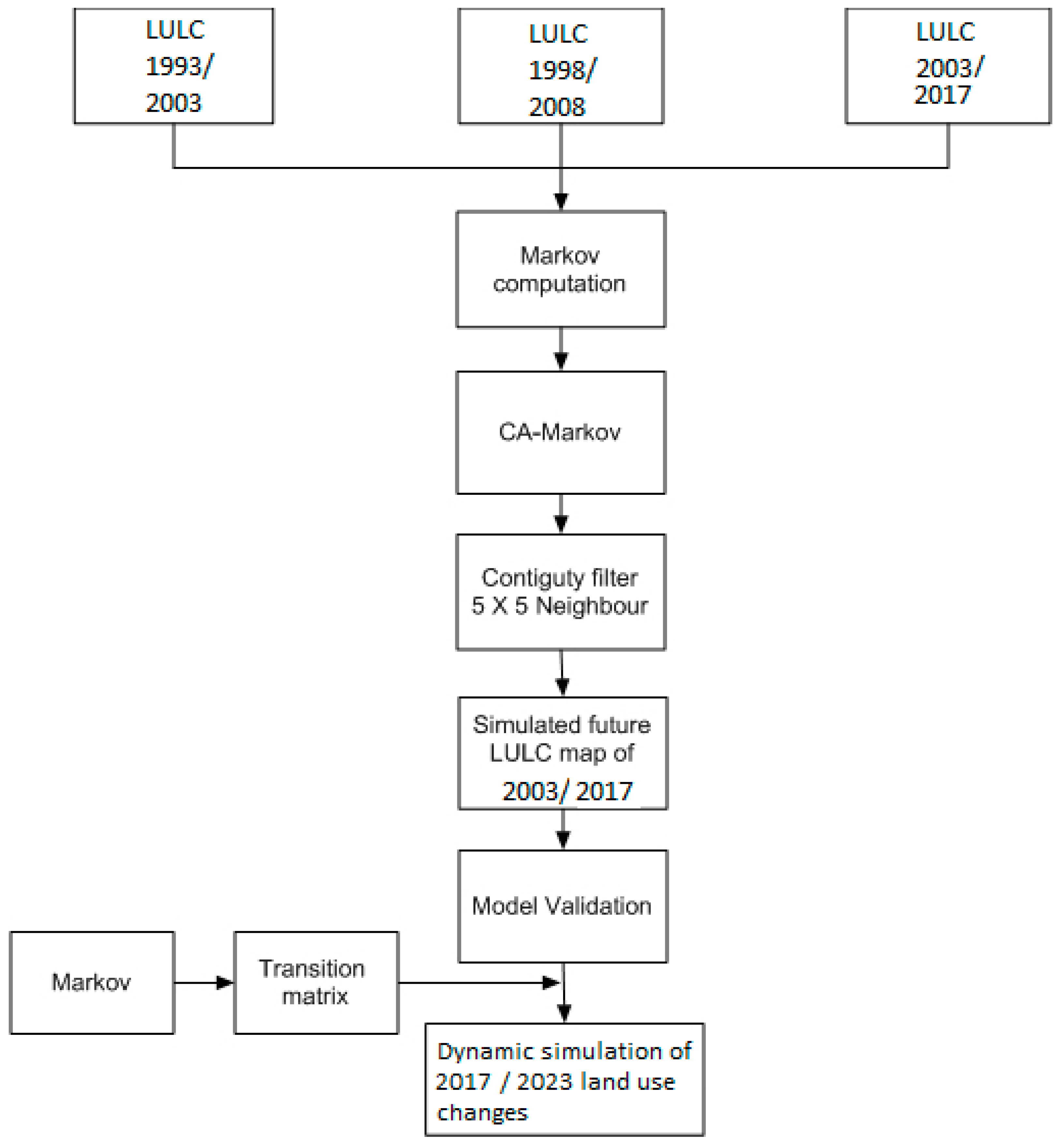
The new political conditions after 2003 were assumed as the second scenario. This period, 2003–2017 represents new socio-economic development that led to substantial improvement in the natural environment. Simultaneously, the images from 2003 and 2008 were used for calibration and optimisation of the Markov chain algorithm, while the image from 2017 was used for validating the predictions of CA-Markov. Like to the first scenario, the land cover map for 2003 is the earliest image (time 1) and 2008 is the latest land cover map (time 2) to simulate the projected 2017 map (time 3), which will be examined against the 2017’s real map. To predict the LULC map in 2023 the Markov and CA-Markov models were used. A flow chart for both scenarios of the applied methodology is shown in Figure 3.

4. Results

4.1. Accuracy Assessment

Table 3. Accuracy assessment for 1993, 1998, 2003, 2008 and 2017 classification.

Land Use/Cover	1993		1998		2003		2008		2017
	P	U	P	U	P	U	P	U	P	U
Bare surface	98	98	97	98	97	99	97	99	98	99
Pasture	97	97	97	98	98	95	97	96	97	97
Cultivated area	96	88	93	96	95	89	94	90	94	92
Forest	96	98	99	96	96	98	97	98	97	98
Overall accuracy	97		97		97		97		97
Overall Kappa Statistic	0.96		0.96		0.96		0.96		0.96

illustrates the producers, users, overall accuracies and kappa statistics of the various LULC classes in the Halgurd-Sakran Core Zone land cover maps for different periods. The results revealed that the overall accuracy and kappa statistics for all classified images were 97% and 0.96 respectively.

4.2. LULC Change Analysis Using LCM

4.2.1. First Scenario

The LULC changes under first scenario conditions were evaluated by gains and losses experienced by different classes using LULC maps of 1993, 1998 and 2003 using change analysis tool available in LCM in TerrSet. Figure 4 shows the gains and losses in LULC in different time periods.

The dark greys indicate the gain per class in km², while the loss of each class shows in the light greys. The bare surface in first scenario has lost 53.85 km² and gained 28.90 km² with net loss of 24.95 km² between 1993 and 1998. Pasture land has the highest amount of gains 51.27 km² and lost 24.92 km² with net gain of 26.35 km². Cultivated land has lost 10.61 km² and gained 5.63 km² with net loss of 4.98 km². Forest has gained 9.85 km² and lost 6.25 km² with net loss of 3.60 km².

During the second period, the bare surface has the highest amount of gains 39.33 km² and it has been lost 30.26 km² with net gain of 9.07 km². Concerning the pasture, the highest surface area lost was 30.37 km² and gain was 29.61 km² with a slight net loss of 0.76 km². Cultivated land has been lost 9.46 km² and gained 5.57 km² with net loss of 3.89 km². Forest land has been lost 11.23 km² and gained 6.81 km² with net loss of 4.42 km². While during the entire third period between 1993 and 2003, bare surface land has the highest amount of loss 48.53 km² and gained 32.65 km² with net loss of 15.88 km². Simultaneously, the highest gains in pasture land was 47.27 km² compared to a loss of 21.69 km² with net gain of 25.58 km². Cultivated land has been lost 14.14 km² and gained 5.26 km² with net loss of 8.88 km². Forest land has been lost 9.16 km² and gained 8.34 km² with a slight net loss of 0.82 km² (Figure 4).

4.2.2. Second Scenario

The LULC changes under second scenario conditions were evaluated by gains and losses experienced by different classes using LULC maps of 2003, 2008 and 2017 using change analysis tool available in LCM in TerrSet. Figure 5 shows the gains and losses in LULC for the second scenario. From 2003 to 2008, the bare surface has gained 37.25 km² and lost 15.04 km². Pasture land has been lost 35.27 km² and gained 14.43 km². Cultivated land has been lost 4.64 km² and gained 9.67 km². Forest land has been lost 11.03 km² and gained 4.63 km². This period represents the time after lifting the sanctions on Iraq and the Fall of Baghdad in April 2003, which witnessed improvements of socio-economic conditions [28].

During the second period (2008–2017), bare surface land has the highest amount of loss 42.36 km² and gained 19.10 km² with net loss of 23.26 km². Pasture land has been gained 43.64 km² and lost 16.70 km² with net gain of 26.94 km². Furthermore, cultivated land has been lost 7.43 km² and gained 6.99 km². Forest land has been gained 4.21 km² and lost 7.45 km² with net loss of 3.24 km². While during the entire third period (between 2003 and 2017), bare surface land has been lost 43.21 km² and gained 38.42 km². Pasture land has been gained 32.74 km² and lost 40 km². Cultivated land has gained 14.17 km² and lost 5.86 km². Forest land has gained 11.54 km² and lost 7.80 km².

4.3. Markov Chain Model Analysis

This procedure contains two significant matrices of probabilities, which are the transition probability matrix and the conditional probability images.

4.3.1. First Scenario

Table 4. Transition probability matrix derived from the land use maps in HSCZ during 1993–1998.

Changing from:	Probability of Changing by 1998 to:				Subtotals
1993	Bare Surface	Pasture	Cultivated Land	Forest	Total	Loss
Bare surface	0.6035	0.3448	0.0206	0.0312	1.00	0.3965
Pasture	0.3158	0.6573	0.0139	0.0130	1.00	0.3427
Cultivated land	0.1682	0.0998	0.5216	0.2104	1.00	0.4784
Forest	0.1313	0.1330	0.1090	0.6267	1.00	0.3733
Total	1.2188	1.2349	0.6651	0.8813	4.00
Gain	0.6153	0.5776	0.1435	0.2546

displays the summary of the probability matrix for major LULC conversions for all classes in HSCZ that took place between 1993 and 1998 of the first scenario. For instance, the probability of change for bare surface to bare surface from 1993 to 1998 is 60.35%, while the probability of future change of bare surface to pasture land is 34.48% and so on for other LULC classes. In the second period (between 1998 and 2003), the probability of change for example, forest to forest is 50.16%, while the probability of future change of forest patch to pasture land is 4.60% (

Table 5. Transition probability matrix derived from the land use maps in HSCZ during 1998–2003.

Changing from:	Probability of Changing by 2003 to:				Subtotals
1998	Bare Surface	Pasture	Cultivated Land	Forest	Total	Loss
Bare surface	0.6900	0.2838	0.0073	0.0189	1.00	0.3100
Pasture	0.2789	0.6606	0.0349	0.0256	1.00	0.3394
Cultivated land	0.3170	0.0468	0.4923	0.1439	1.00	0.5077
Forest	0.3756	0.0460	0.0768	0.5016	1.00	0.4984
Total	1.6615	1.0372	0.6113	0.6900	4.00
Gain	0.9715	0.3766	0.1190	0.1884

).

Row categories in

Table 6. Transition probability matrix derived from the land use maps in HSCZ during 1993–2003.

Changing from:	Probability of Changing by 2003 to:				Subtotals
1993	Bare Surface	Pasture	Cultivated Land	Forest	Total	Loss
Bare surface	0.6279	0.3409	0.0135	0.0178	1.00	0.3721
Pasture	0.2669	0.6823	0.0291	0.0217	1.00	0.3177
Cultivated land	0.3478	0.0514	0.4124	0.1884	1.00	0.5876
Forest	0.3154	0.0825	0.0791	0.5230	1.00	0.4770
Total	1.5580	1.1571	0.5341	0.7509	4.00
Gain	0.9301	0.4748	0.1217	0.2279

characterise LULC classes in 1993 whilst column categories characterise classes of 2003. The pasture land had a probability as high as 68.23% to remain as pasture in 2003. Bare surface land also had a probability as high as 62.79% to remain as barren land in 2003. Concerning the forest and cultivated lands were lesser amount of probability by 52.30% and 41.24% respectively to remain as they are.

The cross-tabulation matrices are represented in Table 4, Table 5 and Table 6 for the first scenario. Tables display the decreasing and increasing of the transition probabilities over three time periods, from 1993 to 1998, 1998 to 2003 and 1993 to 2003. Subtracting the persistence (diagonal entries) from the total column for each group obtains the gain, while subtracting the persistence from the total row for each group obtains the loss.

4.3.2. Second Scenario

Simultaneously, the LULC changes from 2003 to 2008, 2008 to 2017 and 2003 to 2017, cross-tabulation matrices (

Table 7. Transition probability matrix derived from the land use maps in HSCZ during 2003–2008.

Changing from:	Probability of Changing by 2008 to:				Subtotals
2003	Bare Surface	Pasture	Cultivated Land	Forest	Total	Loss
Bare surface	0.7143	0.1889	0.0515	0.0453	1.00	0.2857
Pasture	0.4183	0.5183	0.0484	0.0150	1.00	0.4817
Cultivated land	0.2203	0.2121	0.4283	0.1393	1.00	0.5717
Forest	0.3096	0.1644	0.1745	0.3515	1.00	0.6485
Total	1.6625	1.0837	0.7027	0.5511	4.00
Gain	0.9482	0.5654	0.2744	0.1996

,

Table 8. Transition probability matrix derived from the land use maps in HSCZ during 2008–2017.

Changing from:	Probability of Changing by 2017 to:				Subtotals
2008	Bare Surface	Pasture	Cultivated Land	Forest	Total	Loss
Bare surface	0.7154	0.2501	0.0242	0.0102	1.00	0.2846
Pasture	0.1927	0.7752	0.0207	0.0114	1.00	0.2248
Cultivated land	0.0982	0.1753	0.6329	0.0936	1.00	0.3671
Forest	0.1302	0.1052	0.1053	0.6593	1.00	0.3407
Total	1.1365	1.3058	0.7831	0.7745	4.00
Gain	0.4211	0.5306	0.1502	0.1152

and

Table 9. Transition probability matrix derived from the land use maps in HSCZ during 2003–2017.

Changing from:	Probability of Changing by 2017 to:				Subtotals
2003	Bare Surface	Pasture	Cultivated Land	Forest	Total	Loss
Bare surface	0.7991	0.1572	0.0343	0.0094	1.00	0.2009
Pasture	0.1682	0.8009	0.0231	0.0078	1.00	0.1991
Cultivated land	0.0522	0.1174	0.7334	0.0970	1.00	0.2666
Forest	0.0744	0.1809	0.1008	0.6438	1.00	0.3562
Total	1.0939	1.2564	0.8916	0.7580	4.00
Gain	0.2948	0.4555	0.1582	0.1142

) were developed for the second scenario. Table 7 displays the summary of the probability matrix for major LULC conversions for all classes in HSCZ that took place between 2003 and 2008. The probability of change for bare surface to bare surface is 71.43%, while the pasture land had a probability of 51.83% to remain as pasture land in 2008.

In the second period (between 2008 and 2017), the pasture land had the highest probability of 77. 52% to remain as pasture in 2017. Whereas, the bare surface, cultivated area and forest land had 71.54%, 63.29% and 65.93% respectively, to remain as they are (Table 8). In the third period (2003–2017) of the second scenario, the bare surface had a probability of 79.91% to remain as bare surface in 2017. Pasture land had a probability as high as 80.09% to remain as pasture land in 2017. The forest land had lesser probability of 64.38% to remain as forest land, while the cultivated land had a probability as high as 73.34% to remain as cultivated land (Table 9).

In order to predict the LULC for 2003 and 2017 Markov chain analysis for the time period of 1993–1998 and 2003–2008 were used to calculate the transition probability matrix. In the first scenario, images of 1993 and 2008 of LULC maps were used for developing the transition probability matrix and transition area matrix for year 2003. Concerning for prediction of 2023 the LULC maps for 1993 and 2003 were used (Table 4 and Table 6).

On the other hand, the transition probability matrix and transition area matrix of the second scenario were developed for year 2017 using images 2003 and 2008 of LULC maps. Concerning for prediction of 2023 the LULC maps for 2003 and 2017 were used (Table 7 and Table 9).

4.4. Simulated Future LULC Changes under Different Scenarios

4.4.1. First Scenario

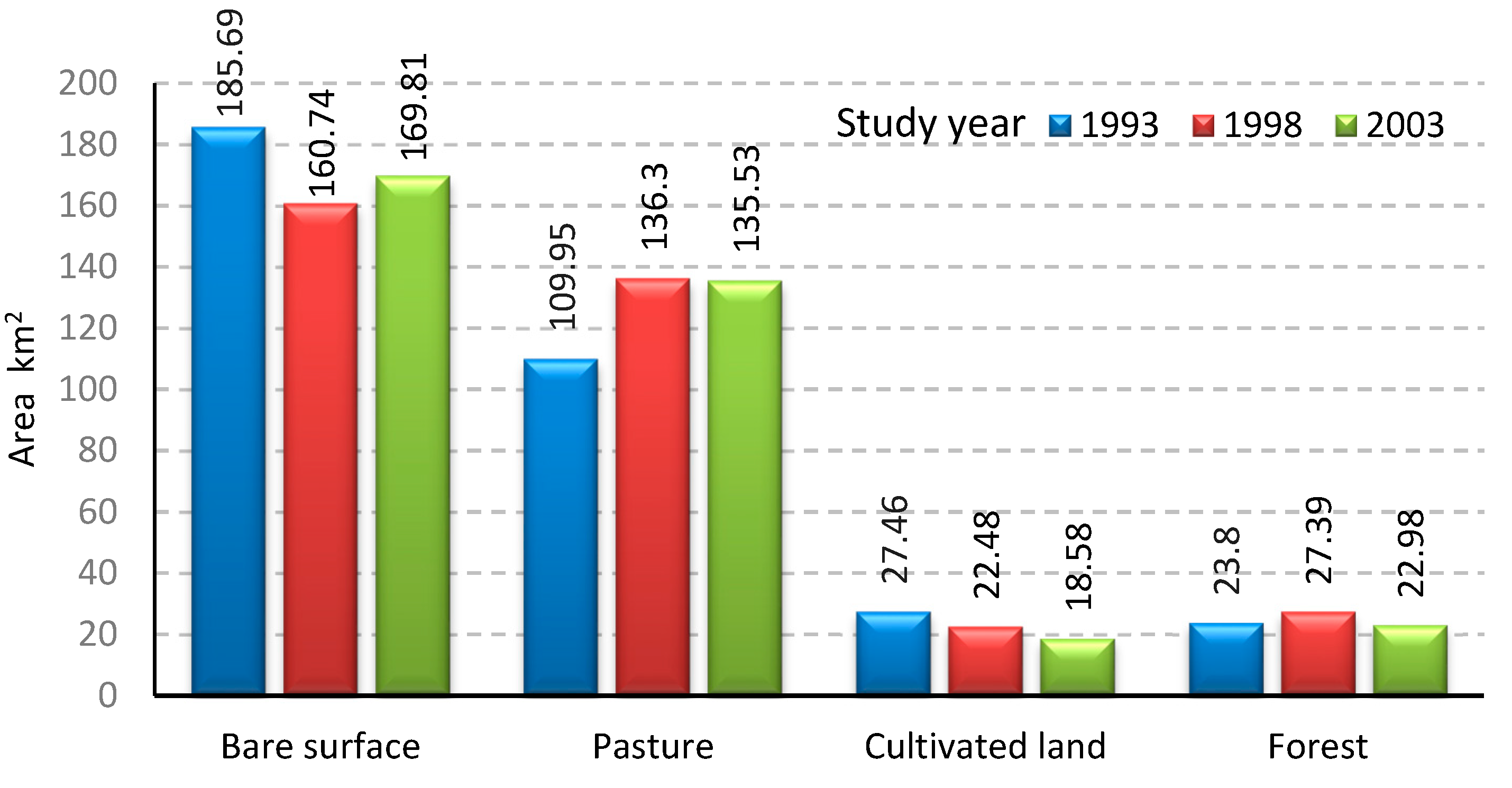
Figure 6 displays the area statistics for all LULC categories during different periods between1993–2003 for the first scenario. During 1993–1998 and 1998–2003 periods bare surface decreased from 185.69 km² to 160.74 km² and then increased to 169.81 km², respectively.

Pasture land has increased between 1993 and 1998 from 109.95 km² to 136.3 km² and then slightly decreased to 135.53 in 2003. There was a continuous reduction of cultivated land from 27.46 km² in 1993 to 22.48 km² in 1998 and then to 18.58 km² in 2003. The forest land increased slightly from 23.80 km² in 1993 to 27.39 km² in 1998 and then decreased to 22.98 km² in 2003.

The reduction of cultivated land can be associated with the period of implying the “Oil-Food-Program” that improved somewhat the socio-economic change. Furthermore, “The first Iraqi oil under the Oil-for-Food Programme was exported in December 1996 and the first shipments of food arrived in March 1997” [11]. Figure 7 display areas for simulated 2003 and real 2003 maps in square kilometres for land use/land cover classes in the HSCZ of the National park.

The reference and simulated maps for year 2003 were reasonably comparable or close especially for cultivated land, while for the rest of LULC there were differences between simulated and real maps.

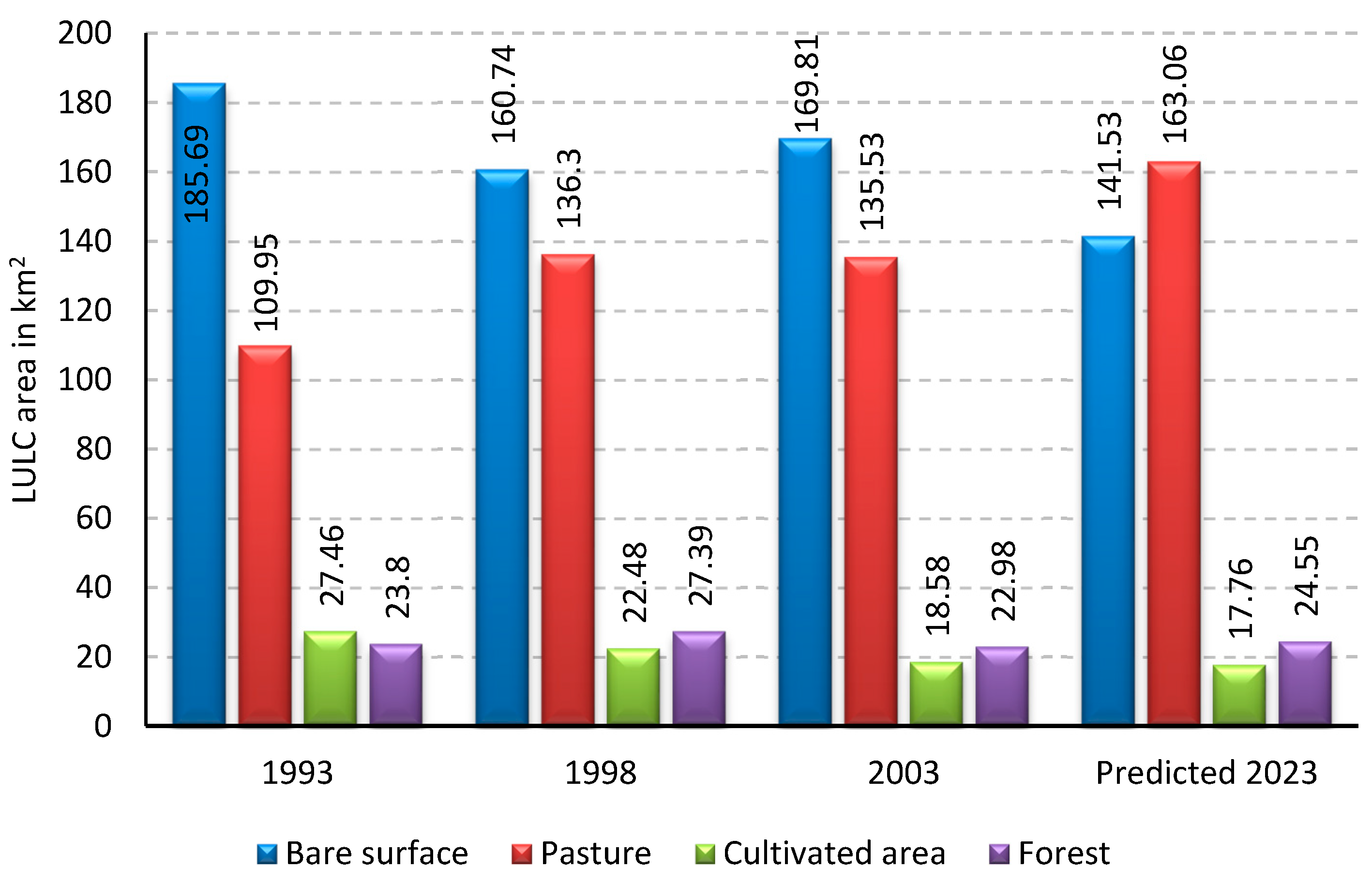
A stronger agreement is indicated when the indices reach 100%. The poor results for any class indicate that these class matrices did not predict any changes for 2003. The real 1998 LULC map was used as the base map for estimating future LULC scenario for 2023 using CA-Markov model. In this regard, Markov and Cellular Automata used to predict for 2023 as future changes of LULC. The predicted LULC for 2023 indicates that the net percentage estimate would be 141.53, 163.06, 17.76 and 24.55 km for bare surface, pasture, cultivated and forest-lands, respectively in HSCZ (

Table 10. The predictability areas of 2023 for LULC classes under sanctions (first scenario) in square kilometres.

LULC Classes	Projected 2023 in km2
Barren land	141.53
Pasture land	163.06
Cultivated land	17.76
Forest land	24.55
Total	346.9

). Figure 8 displays the projected 2023 of LULC classes of the study area assumed under the continuing sanctions on Iraq.

4.4.2. Second Scenario

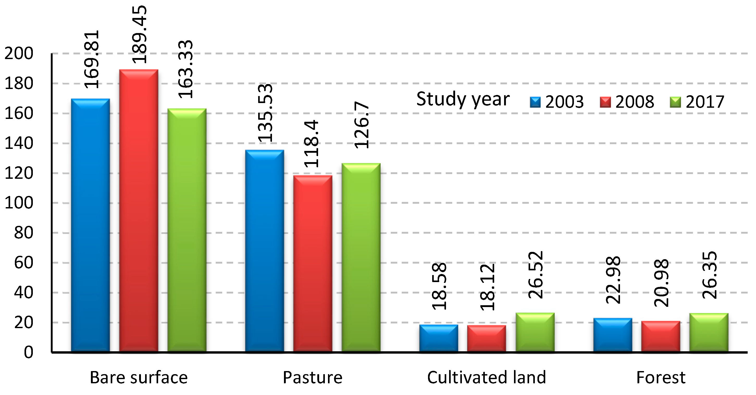
Concerning the second scenario bare surface increased from 169.81 km² in 2003 to 189.45 in 2008 and then after, started to decrease 163.33 km² in 2017. Pasture land decreased from 135.53 to 118.4 between 2003 and 2008 and then after increased to dominate 126.70 km² of the entire area of the HSCZ in 2017. Cultivated land was almost stable between 2003 and 2008 and then after increased to 26.52 km² in 2017. Forest area decreased from 22.98 km² in 2003 to 20.98 in 2008 and then after, started to increase 26.35 km² in 2017, Figure 9.

Figure 10 displays areas for simulated 2017 and real 2017 in square kilometres and for LULC classes in the HSCZ of the National park. The reference and simulated maps for year 2017 were reasonably similar for forest land, while for the other LULC classes there were almost slight differences between simulated and real maps. Figure 11 shows the projected 2023 map of LULC classes of the second scenario, whereas

Table 11. The predictability areas of 2023 for LULC classes after sanctions (second scenario) in square kilometres.

LULC Classes	Projected 2023 in km2
Bare surface	162.46
Pasture land	133.19
Cultivated land	23.97
Forest land	27.28
Total	346.94

displays the predictability areas of 2023, after rising the sanctions.

4.5. Model Validation

Concerning the model validation and based on the comparison of predicted LULC of 2003 with actual LULC map of 2003 for the first scenario, the κ coefficient for quantity and location was derived. The statistics show that κ_no is 0.8866, κ_location is 0.8805, κ_{location strata} is 0.8805 and κ_standard is 0.8269 (overall κ), respectively. Thus, there are almost no or small quantification and location errors. The simulation for this scenario has perfect ability to specify location accurately and it also has perfect ability to specify quantity accurately. For validation purpose, Kappa Index of Agreement (κ_IA) was used for predicting the LULC map of 2003.

Table 12. κ for 2003 and 2017.

κ Indicators	2003	2017
κno	0.8866	0.8318
κlocation	0.8805	0.8936
κlocationStrata	0.8805	0.8543
κstandard	0.8269	0.8543

confirmed that the accuracy assessment of the classified data of 2003 is acceptable and reasonable for any applications based on κ_IA. All κ index values exceed the minimum acceptable standard and they were greater than 80%, showing good agreement between predicted and actual LULC map [19,55].

On the other hand, the statistics in the second scenario for κ_no, κ_location, κ_{locationStrata} and κ_standard predicted LULC of 2017 were 0.8318, 0.8936, 0.8543 and 0.8543 (overall κ), respectively. All κ_IA values showed also a very good agreement between projected and actual LULC map. Hence, all values are greater than 80% for both scenarios, which proves that the Markov simulation model was well designed and the accuracy assessment was sufficiently accurate especially, for simulated map of 2017. Simultaneously, the simulation for the second scenario has also excellent ability to specify location accurately and quantity accurately.

5. Discussion

This study presents CA-Markov model of LULC change that provides an answer to the research question of where LULC changes are expected to occur under two business-as-usual scenarios. The first scenario describes a historical LULC change that was observed between 1993 and 2003 under the sanction period, which represents a period of economic conflict in the form of a comprehensive set of sanctions.

However, the second scenario of the BAU assumption examines the period of new political conditions and economic development that led to substantial improvement in the natural environment. Moreover, the current research was conducted without taking into consideration any driver forces that are playing an influential role in the land use changes because data and documentation were limited. Therefore, the scenario models reflect only the surrounding natural environment.

The overall results of LULC distribution for the predicted map in 2023 in the first scenario showed that the pasture land was the primary dominant land cover category. Meanwhile, bare surface class was the dominant class in the second scenario (Figure 12).

5.1. LULC Change Analysis Using LCM

All kappa index values in Table 12 are greater than 0.8, which indicates good agreement between predicted and observed LULC maps. A Markov chain model was used in both scenarios for predicting the state of 2023 (Figure 8 and Figure 11).

5.1.1. First Scenario

The first scenario would represent the period within the continuous sanction from 1993. The prediction has been conducted for 2023 based on BAU assumption, which sanction would have had continued. The spatial patterns of the predicted LULC map showed that there would be a decrease of bare surface and an increase of the pasture from 2003 to 2023. The cultivated land would decrease from 2003 to the 2023, simultaneously forest land would increase in the HSCZ. The decrease of cultivated area from 2003 to 2023 can be attributed by the leaving people their places in rural areas and started moving to the sub-districts or districts, as rural areas will likely face a higher risk of poverty and lower incomes compared with urban areas under siege (Figure 13). Though, the natural resources in HSCZ will grow without destroying or over-exploiting the environment or the ecosystems. Thus, the natural resources remain diverse and productive over long periods of time. Furthermore, this can help to reduce the impacts of agriculture on natural environment, increasing the pasture land and preventing soil degradation and erosion.

Additionally, these prediction trends of LULC classes can be combined with increasing environmental involvement. Then again, the trends and predictions of the decreasing bare surface and increasing pasture land from 2003 to 2023 in HSCZ would have a serious impact on improving the ecosystem services and the rich biodiversity.

The period from 1993 to 2003 visualise a continuous decrease of cultivated land. High amount of area has been used in 1993 by farmers as a result of food demand and low income, which represents the start period of siege on Iraq. In 1998 the cultivated land has been decreased, which can be linked to the applying the “Oil-Food-Program” that started in December 1996 [11]. In this period, people lived in a better condition and used lesser area for land use as a result of better sustenance. After lifting the siege or after the Fall of Baghdad the cultivated area continued to decline, which indicates the improvement of life and economic boom.

Moreover, a slight increase can be observed of forest land between 1993 and 1998. This can be explained and associated with also the “Oil-Food-Program.” People stopped logging off the forest for temporary period. The inhabitants started again logging off trees after 1998 and the area of forest in the HSCZ decreased until 2003. From 1993 and 2003 a dynamic of bare surface can be identified in a heterogeneous landscape in HSCZ. The spatial pattern of the study area showed that there had been a steady increase in pasture land area from 1993 and 1998, while it decreased from 1998 to 2003. After the lifting of the sanctions on Iraq a steady increase in pasture land can be observed. Decreasing the bare surface and increasing the pasture land in the study area, especially in the steep areas, is reflected in the reduction of ecological problems including the decreasing of soil erosion and mudslides.

5.1.2. Second Scenario

Meanwhile, the predicted LULC for 2023 of the second scenario indicates that the net percentage estimate would be 162.46, 133.19, 23.97 and 27.28 km² for bare surface, pasture, cultivated and forest-lands, respectively in HSCZ (Figure 14). Moreover, the simulation scenario for year 2023 showed that there would be a slight decrease by 0.13 km² in the bare surface and a continuous increase in pasture area between 2017 and 2023. The cultivated area would decrease by 2.55 km², while there would be an increase of the forest patch from 2017 to 2023 by 0.93 km². Furthermore, the rate changes of predicted bare surface and pasture land were higher in first scenario compared to second scenario. Whereas, the rate of cultivated and forest land in both scenarios were almost lower.

Most bare surface in HSCZ covers the top of mountains [28]. Therefore, decreasing the rate of bare surface land formation leads to increasing in the infiltration and decreasing in the amount of runoff, which decreases the displacement of the upper layer of the soil during rainfall.

As a result, the model suggests that pasture land would suffer less erosion and the productivity would be improved by increasing of natural pasture in Halgurd-Sakran National Park in next 6 years. Forest land would increase in the park. Expanding the forest resources is the first measure of sustainable forest management. Decreasing barren land means that it would turn into forest, pasture or cultivated areas. The prediction of decreasing the cultivated land from 2017 to 2023 might be expected to the increases in socio-economic boom, which represents the period after siege.

In this study, the following factors were not considered: geophysical, climatic, socio-economic, distance to housing and road networks due to the lack of data availability. However, absence of these factors may cause differences in simulation results of land use structure. Therefore, further investigations are required through the implementation of each scenario (physical, economic and human factors as mentioned in Section 1) into different modelling and comparing between each model outputs at various spatial scales. In general, scenarios are intended to provide decision makers to have a control and monitor the potential occasions and challenges that future circumstances may possibly present.

Finally, this study was carried out based on the statistical independence test and validity of the CA-Markov process for predicting future LULC changes. A reliable forecast, is generating the model processing into the future or to the past [21] to better understand the dynamics of systems, make predictions and evaluate scenarios for use in assessment activities [16]. The overall findings from the general results indicate that the United Nations sanctions on Iraq had the greatest impact on cultivated area in HSCZ.

6. Conclusions

Using the combined Markov and Cellular Automata future changes of LULC has been predicted for 2023 under two different scenarios. In this study, we quantified landscape changes using LCM in TerrSet over a 30-year period in Halgurd-Sakran Core Zone. Dynamics of LULC changes under two different scenarios to predict the future spatial and temporal changes in the year 2023 in HSCZ has been carried out using geospatial technology. Furthermore, we created a transition matrix that easily shows the transition from one category to another during all time intervals. Multi-temporal Landsat imagery of 1993, 1998, 2003, 2008 and 2017 were used to derive LULC maps which were further used in the CA-Markov process to successfully predict the future spatial and temporal changes of LULC. An accuracy of more than 80% was obtained in all stages. Different results obtained from two different scenarios. Thus CA-Markov modelling has provided promisingly accurate and reliable results in this study. Furthermore, this study showed the versatility of remote sensing, GIS and LULC change model that can be used as an efficient tool for mapping and monitoring the alterations of LULC.

In general, the weaknesses inherent in traditional methods are that they do not account for environmental, social or demographic conditions. Researchers would have to combine these models in order to overcome this shortage. For instance, combining the CA-Markov, the multi-criteria evaluation (MCE) and analytic hierarchy process (AHP), would improve the demonstration of the dynamic growth in urban areas.

Overall findings, the sanctions had significant impact on agricultural areas in HSCZ. Furthermore, the natural environment of the park during Iraq under sanctions in the first scenario was more stable compared to the natural environment during Iraq after lifting the sanction in the second scenario. This type of prediction of future LULC image can be helpful in the field of management of natural resources.

References

- Roy, S.; Farzana, K.; Papia, M.; Hasan, M. Monitoring and prediction of land use/land cover change using the integration of Markov chain model and cellular automation in the Southeastern Tertiary Hilly Area of Bangladesh. Int. J. Sci. Basic Appl. Res. 2015, 24, 125–148. [Google Scholar]
- Meles, K.H. Temporal and Spatial Changes in Land Use Patterns and Biodiversity in Relation to Farm Productivity at Multiple Scales in Tigray, Ethiopia; Wageningen Universiteit: Wageningen, The Netherlands, 2008. [Google Scholar]
- Hamad, R.; Kolo, K.; Balzter, H. Land Cover Changes Induced by Demining Operations in Halgurd-Sakran National Park in the Kurdistan Region of Iraq. Sustainability 2018, 10, 2422. [Google Scholar] [CrossRef]
- Singh, S.K.; Mustak, S.; Srivastava, P.K.; Szabó, S.; Islam, T. Predicting spatial and decadal LULC changes through cellular automata Markov chain models using earth observation datasets and geo-information. Environ. Process. 2015, 2, 61–78. [Google Scholar] [CrossRef]
- Ali, H. Land Use and Land Cover Change, Drivers and Its Impact: A Comparative Study from Kuhar Michael and Lenche Dima of Blue Nile and Awash Basins of Ethiopia; Cornell University: New York, NY, USA, 2009. [Google Scholar]
- Gibson, G.R. War and Agriculture: Three Decades of Agricultural Land Use and Land Cover Change in Iraq; University Libraries, Virginia Polytechnic Institute and State University: Blacksburg, VA, USA, 2012. [Google Scholar]
- Dezhkam, S.; Amiri, B.J.; Darvishsefat, A.A.; Sakieh, Y. Performance evaluation of land change simulation models using landscape metrics. Geocarto Int. 2017, 32, 655–677. [Google Scholar] [CrossRef]
- Regmi, R.; Saha, S.; Balla, M. Geospatial analysis of land use land cover change predictive modeling at Phewa Lake Watershed of Nepal. Int. J. Curr. Eng. Tech. 2014, 4, 2617–2627. [Google Scholar]
- Omar, N.Q.; Sanusi, S.A.; Hussin, W.M.; Samat, N.; Mohammed, K.S. Markov-CA model using analytical hierarchy process and multiregression technique. In IOP Conference Series: Earth and Environmental Science; IOP Publishing: Bristol, UK, 2014. [Google Scholar]
- Hamad, R.; Kolo, K.; Balzter, H. Post-war land cover changes and fragmentation in Halgurd Sakran National Park (HSNP), Kurdistan region of Iraq. Land 2018, 7, 38. [Google Scholar] [CrossRef]
- United Nations-Office of the Iraq Programme_Oil-for-Food Programme. Available online: http://www.un.org/Depts/oip/background/ (accessed on 25 April 2018).
- Lortz, M.G. Willing to Face Death: A History of Kurdish Military Forces—The Peshmerga—From the Ottoman Empire to Present-Day Iraq; Florida State University: Tallahassee, FL, USA, 2005. [Google Scholar]
- Olmedo, M.T.C.; Pontius, R.G., Jr.; Paegelow, M.; Mas, J.-F. Comparison of simulation models in terms of quantity and allocation of land change. Environ. Model. Softw. 2015, 69, 214–221. [Google Scholar] [CrossRef] [Green Version]
- Liu, Y.; Dai, L.; Xiong, H. Simulation of urban expansion patterns by integrating auto-logistic regression, Markov chain and cellular automata models. J. Environ. Plan. Manag. 2015, 58, 1113–1136. [Google Scholar] [CrossRef]
- Fan, F.; Weng, Q.; Wang, Y. Land use and land cover change in Guangzhou, China, from 1998 to 2003, based on Landsat TM/ETM+ imagery. Sensors 2007, 7, 1323–1342. [Google Scholar] [CrossRef]
- Brown, D.G.; Walker, R.; Manson, S.; Seto, K. Modeling land use and land cover change. Land Chang. Sci. 2004. [Google Scholar] [CrossRef]
- Land Change Modeler in TerrSet. Available online: https://clarklabs.org/terrset/land-change-modeler/ (accessed on 25 May 2018).
- Megahed, Y.; Cabral, P.; Silva, J.; Caetano, M. Land cover mapping analysis and urban growth modelling using remote sensing techniques in greater Cairo region—Egypt. ISPRS Int. J. Geo-Inf. 2015, 4, 1750–1769. [Google Scholar] [CrossRef]
- Mishra, V.N.; Rai, P.K.; Mohan, K. Prediction of land use changes based on land change modeler (LCM) using remote sensing: A case study of Muzaffarpur (Bihar), India. J. Geogr. Inst. Jovan Cvijic SASA 2014, 64, 111–127. [Google Scholar] [CrossRef]
- Krishna Rajan, D. Understanding the Drivers Affecting Land Use Change in Ecuador: An Application of the Land Change Modeler Software. Available online: https://www.era.lib.ed.ac.uk/handle/1842/3740 (accessed on 17 September 2018).
- Veldkamp, A.; Lambin, E.F. Predicting land-use change. Agr. Ecosyst. Environ. 2001, 85, 1–6. [Google Scholar] [CrossRef]
- Moulds, S.; Buytaert, W.; Mijic, A. An open and extensible framework for spatially explicit land use change modelling: The lulcc R package. Geosci. Model Dev. 2015, 8, 3215–3229. [Google Scholar] [CrossRef]
- Ozturk, D. Urban growth simulation of atakum (Samsun, Turkey) using cellular automata-Markov chain and multi-layer perceptron-markov chain models. Remote Sens. 2015, 7, 5918–5950. [Google Scholar] [CrossRef]
- Parsa, V.A.; Yavari, A.; Nejadi, A. Spatio-temporal analysis of land use/land cover pattern changes in Arasbaran Biosphere Reserve: Iran. Model. Earth Syst. Environ. 2016, 2, 1–13. [Google Scholar] [CrossRef] [Green Version]
- Mondal, M.S.; Sharma, N.; Garg, P.K.; Kappas, M. Statistical independence test and validation of CA Markov land use land cover (LULC) prediction results. Egypt. J. Remote Sens. Space Sci. 2016, 19, 259–272. [Google Scholar] [CrossRef]
- The USGS Global Visualization Viewer. Available online: https://glovis.usgs.gov/ (accessed on 15 May 2018).
- The R Project for Statistical Computing. 2013. Available online: http://www.R-project.org/ (accessed on 15 July 2018).
- Hamad, R.; Balzter, H.; Kolo, K. Multi-criteria assessment of land cover dynamic changes in halgurd sakran national park (HSNP), kurdistan region of Iraq, using remote sensing and GIS. Land 2017, 6, 18. [Google Scholar] [CrossRef]
- Congalton, R.G.; Green, K. Assessing the Accuracy of Remotely Sensed Data: Principles and Practices; CRC Press: Boca Raton, FL, USA, 2008. [Google Scholar]
- TerrSet Geospatial Monitoring and Modeling System-Manual. Available online: https://clarklabs.org/wp-content/uploads/2016/10/Terrset-Manual.pdf/ (accessed on 5 May 2018).
- Weng, Q. Land use change analysis in the Zhujiang Delta of China using satellite remote sensing, GIS and stochastic modelling. J. Environ. Manag. 2002, 64, 273–284. [Google Scholar] [CrossRef] [Green Version]
- Nouri, J.; Gharagozlou, A.; Arjmandi, R.; Faryadi, S.; Adl, M. Predicting urban land use changes using a CA–Markov model. Arab. J. Sci. Eng. 2014, 39, 5565–5573. [Google Scholar] [CrossRef]
- Hua, A. Application of Ca-Markov model and land use/land cover changes in Malacca River Watershed, Malaysia. Appl. Ecol. Environ. Res. 2017, 15, 605–622. [Google Scholar] [CrossRef]
- Ghosh, P.; Mukhopadhyay, A.; Chanda, A.; Mondal, P.; Akhand, A.; Mukherjee, S.; Nayak, S.K.; Ghosh, S.; Mitra, D.; Ghosh, T.; et al. Application of Cellular automata and Markov-chain model in geospatial environmental modeling—A review. Remote Sens. Appl. Soc. Environ. 2017, 5, 64–77. [Google Scholar] [CrossRef]
- Yang, X.; Zheng, X.-Q.; Chen, R. A land use change model: Integrating landscape pattern indexes and Markov-CA. Ecol. Model. 2014, 283, 1–7. [Google Scholar] [CrossRef]
- Subedi, P.; Subedi, K.; Thapa, B. Application of a hybrid cellular automaton-Markov (CA-Markov) Model in land-use change prediction: A case study of saddle creek drainage Basin, Florida. Appl. Ecol. Environ. Sci. 2013, 1, 126–132. [Google Scholar] [CrossRef]
- Burnham, B.O. Markov intertemporal land use simulation model. J. Agric. Appl. Econ. 1973, 5, 253–258. [Google Scholar] [CrossRef]
- Kumar, S.; Radhakrishnan, N.; Mathew, S. Land use change modelling using a Markov model and remote sensing. Geomat. Nat. Hazards Risk 2014, 5, 145–156. [Google Scholar] [CrossRef]
- D Behera, M.; Borate, S.N.; Panda, S.N.; Behera, P.R.; Roy, P.S. Modelling and analyzing the watershed dynamics using Cellular Automata (CA)-Markov model—A geo-information based approach. J. Earth Syst. Sci. 2012, 121, 1011–1024. [Google Scholar] [CrossRef]
- Sang, L.; Zhang, C.; Yang, J.; Zhu, D.; Yun, W. Simulation of land use spatial pattern of towns and villages based on CA–Markov model. Math. Comput. Model. 2011, 54, 938–943. [Google Scholar] [CrossRef]
- Turner, M.G. Landscape ecology: The effect of pattern on process. Annu. Rev. Ecol. Syst. 1989, 20, 171–197. [Google Scholar] [CrossRef]
- Nadoushan, M.A.; Soffianian, A.; Alebrahim, A. Modeling land use/cover changes by the combination of markov chain and cellular automata markov (CA-Markov) models. J. Earth Environ. Health Sci. 2015, 1, 16–21. [Google Scholar] [CrossRef]
- Eastman, J.R. TerrSet manual. Access. TerrSet Vers. 2015, 18, 1–390. [Google Scholar]
- Wang, Y.; Zhang, X. A dynamic modeling approach to simulating socioeconomic effects on landscape changes. Ecol. Model. 2001, 140, 141–162. [Google Scholar] [CrossRef]
- Pontius, G.R.; Malanson, J. Comparison of the structure and accuracy of two land change models. Int. J. Geogr. Inf. Sci. 2005, 19, 243–265. [Google Scholar] [CrossRef]
- Ye, B.; Bai, Z. Simulating land use/cover changes of Nenjiang County based on CA-Markov model. Comput. Comput. Technol. Agric. 2008, 1, 321–329. [Google Scholar]
- Reddy, C.S.; Singh, S.; Dadhwal, V.K.; Jha, C.S.; Rao, N.R.; Diwakar, P.G. Predictive modelling of the spatial pattern of past and future forest cover changes in India. J. Earth Syst. Sci. 2017, 126. [Google Scholar] [CrossRef]
- Ahmed, B. Land Cover Change Prediction of Dhaka City: A Markov Cellular Automata Approach. 2011. Available online: http://discovery.ucl.ac.uk/1419016/ (accessed on 26 August 2018).
- Adhikari, S.; Southworth, J. Simulating forest cover changes of Bannerghatta National Park based on a CA-Markov model: A remote sensing approach. Remote Sens. 2012, 4, 3215–3243. [Google Scholar] [CrossRef]
- Mandal, U.K. Geo-information Based Spatio-temporal Modeling of Urban Land Use and Land Cover Change in Butwal Municipality, Nepal. Int. Arch. Photogramm. Remote Sens. Spat. Inf. Sci. 2014, 40, 809. [Google Scholar] [CrossRef]
- Chen, L.; Nuo, W. Dynamic simulation of land use changes in Port city: A case study of Dalian, China. Procedia Soc. Behav. Sci. 2013, 96, 981–992. [Google Scholar] [CrossRef]
- Pontius, R.G.; Schneider, L.C. Land-cover change model validation by an ROC method for the Ipswich watershed, Massachusetts, USA. Agric. Ecosyst. Environ. 2001, 85, 239–248. [Google Scholar] [CrossRef]
- Sayemuzzaman, M.; Jha, M. Modeling of future land cover land use change in North Carolina using Markov chain and cellular automata model. Am. J. Eng. Appl. Sci. 2014, 7, 295–306. [Google Scholar] [CrossRef]
- Pontius, R.G. Quantification error versus location error in comparison of categorical maps. Photogramm. Eng. Remote Sens. 2000, 66, 1011–1016. [Google Scholar]
- Eastman, J.R. IDRISI Andes Tutorial; Clark Labs: Worcester, MA, USA, 2006. [Google Scholar]
- Samie, A.; Deng, X.; Siqi, J.; Chen, D. Scenario-based simulation on dynamics of land-use-land-cover change in Punjab Province, Pakistan. Sustainability 2017, 9, 1285. [Google Scholar] [CrossRef]
- Singh, A.K. Modelling Land Use Land Cover Changes Using Cellular Automata in a Geo-Spatial Environment; International Institute for Geo-information Science and Earth Observation: Enschede, The Netherlands, 2003; Available online: https://pdfs.semanticscholar.org/b8b3/5045349ac793a98605ba4c0710c11b76aed3.pdf (accessed on 17 September 2018).
Figure 1.
Geographical location of Halgurd-Sakran Core Zone.
Figure 2.
Land use/land cover distribution maps of HSCZ from classification using the random forest package in R with all spectral bands, elevation, slope, aspect and NDVI band input and training data for each class of Landsat images in five different periods: (a) 1993 (TM 5); (b) 1998 (TM 5); (c) 2003 (TM 5); (d) 2008 (TM 5) and (e) 2017 (OLI 8).
Figure 3.
Flowchart of the methodology implemented for first and second scenarios.
Figure 4.
Gains and losses in km2 of LULC by category in different time periods. Dark and light grey are indication of gain and loss respectively.
Figure 5.
Figure 6.
Area Statistics of Actual LULC classes for the years 1993, 1998 and 2003 in square kilometres.
Figure 7.
The comparison between simulated map (blue colour) and real map (red colour) in square kilometres of 2003 in HSCZ.
Figure 8.
Projected land cover under sanctions, first scenario for 2023 of HSCZ.
Figure 9.
Area Statistics of Actual LULC classes (second scenario) in square kilometres for the years 2003, 2008 and 2017.
Figure 10.
The comparison between simulated map (blue colour) and real map (orange colour) of 2017 in HSCZ.
Figure 11.
Projected land cover, second scenario for 2023 of HSCZ.
Figure 12.
The comparison of LULC area classes under two business-as-usual scenarios in square kilometres.
Figure 13.
Area changes in square kilometres of land use/cover classes for years 1993, 1998, 2003 and predicted 2023 of HSCZ.
Figure 14.
Area changes in square kilometres of land use/cover classes for years 2003, 2008, 2017 and predicted 2023, (second scenario) of HSCZ.