Carbon Emission Performance of Independent Oil and Natural Gas Producers in the United States

Business School, China University of Political Science and Law, Beijing 100088, China
*
Author to whom correspondence should be addressed.
Sustainability 2018, 10(1), 110; https://doi.org/10.3390/su10010110
Submission received: 16 October 2017
/
Revised: 30 December 2017
/
Accepted: 1 January 2018
/
Published: 8 January 2018
(This article belongs to the Section Energy Sustainability)
Abstract
:The oil and natural gas producers have undergone a lot of pressures to curb their carbon emissions as part of the global efforts to address the climate change problem. This paper aims to examine the carbon emission performance of a set of independent oil and natural gas producers in the United States for the period 2011–2015. For each producer, we manually collect its drilling, oil production and gas production data from the annual reports, and extract the carbon emissions data from the EPA’s Greenhouse Gas Reporting Program (GHGRP). We develop empirical models based on the data envelopment analysis (DEA) approach and the Malmquist index measurement. The proposed DEA models generate unified efficiency scores to capture the carbon emission performance under natural disposability and managerial disposability respectively. Then the DEA-based Malmquist indexes are derived to measure the change of carbon emission performance over time. We are able to identify climate leaders and laggards among the producers. Furthermore, we find that the performance has improved from 2012 to 2015 under natural disposability. Under managerial disposability, the indexes exhibit significantly greater dispersions than the indexes under natural disposability, and there is an industry-wide loss of efficiency in terms of technical change. The sustainable development of the independent oil and gas producers requires them to invest more in emission mitigation measures, such as energy conservation, leak detection and repair, flaring reduction, and even renewable energy.
Keywords:
climate change; oil; natural gas; efficiency; drilling; corporate sustainability; DEA; Malmquist index1. Introduction
Business leaders, policymakers and researchers have reached a consensus that limiting the carbon emissions from the oil and natural gas industry is an important task in coping with the challenge of climate change [1,2]. Consequently, the industry has undergone a lot of pressures to take actions to mitigate the carbon emissions [3]. In this study, we aim to assess the carbon emission performance of a group of independent oil and natural gas producers in the United States (US). The independent producers refer to those that mainly operate in the upstream exploration and production sector of the petroleum value chain, with little or no downstream refining or marketing business. The purpose of the study is to obtain comparative results both among the producers and across the time horizon. Specifically, we aim to answer the following two research questions. First, which independent producers are the leaders in terms of carbon emission performance and which are the laggards? Second, how does the carbon emission performance evolve over time? Has the performance improved or deteriorated?
It is estimated that in the US, the entire oil and natural gas industry emits about 224 million metric tons (MMT) of carbon dioxide equivalent (CO2e), of which around 100 MMT emissions are from the production sector [4]. In oil and gas production operations, carbon emissions are mainly attributed to combustion, equipment leaks and venting [5]. Combustion-related emissions arise primarily from burning of fuel to drive the equipment and flaring. Flaring, as a routine practice in the industry, refers to the combustion of associated gas that is produced alongside the oil but cannot be captured and used due to technical, safety and economic reasons. Equipment leaks refer to the unintentional fugitive emissions resulted from equipment failure and damage. Venting refers to the intentional release of natural gas designed into the the equipment or system. The oil and natural gas producers may choose to reduce carbon emissions by adopting green technologies and practices. A set of methods are available for the producers to curb carbon emissions from their operations. For instance, a typical method called “green completion” or “reduced emissions completion” can capture the natural gas that would otherwise escape into the air during a well-completion stage [6]. But there is a tradeoff between cost and environmental benefit. The American Petroleum Institute estimates that the green completion method costs $180,000 per well [7].
Figure 1 shows the total carbon emissions from onshore and offshore oil/gas production for 2011–2015. The data are extracted and compiled from the EPA’s GHG Reporting Program (GHGRP), which monitors the facilities emitting more than 25,000 metric tons of CO2e per year (Link to GHGRP: https://www.epa.gov/ghgreporting, accessed on 20 September 2017). The left panel depicts the emissions by production sites. The right panel indicates the top 15 emitting companies. We can see that production is concentrated in several states/regions, most notably in Texas, Oklahoma, and the Mexican Gulf. The biggest emitting producer is Conoco Phillips (Houston, TX, USA), which emits significantly more carbon than the second one, ExxonMobil Corporation (Irving, TX, USA). Both Conoco Phillips (Houston, TX, USA) and ExxonMobil (Irving, TX, USA) are integrated companies that engage in exploration, production, refinement and distribution. Chesapeake Energy Corporation (Oklahoma City, OK, USA), an independent producer, comes at the third place, emitting 24.1 MMT. While on average the integrated companies generate more carbon emissions than independent producers, the overall emissions from independent producers are larger. Figure 2 shows the annual emissions from integrated and independent companies in the upstream production sector from 2011 to 2015, with data obtained from GHGRP. The figure indicates that independent producers consistently generate more than three quarters of the total emissions in the production sector. In this study we focus on the independent producers. Integrated companies (e.g., BP (London, UK), Chevron (San Ramon, CA, USA), Conoco Phillips (Houston, TX, USA), ExxonMobil (Irving, TX, USA)) are excluded from analysis, because their other operations (e.g., refinement and distribution) make it difficult to compare them with independent producers.
For the purpose of performance measurement, we propose the application of the data envelopment analysis (DEA) and the Malmquist index method to the oil and gas producers. The proposed DEA method has several advantages over other methods in production economics. First, the method can model the oil and gas production business as a multi-input and multi-output procedure, and thus yield a more comprehensive assessment than traditional ratio analysis based on single input and single output. Second, it incorporates the concepts of natural disposability and managerial disposability. Here, natural disposability refers to the scenario that a producer can reduce carbon emissions by cutting back its drilling activity, and managerial disposability refers to the scenario that a producer can increase the drilling activity and reduce carbon emissions simultaneously through managerial efforts. The conceptual and methodological distinctions of natural/managerial disposability from the most widely used weak/strong disposability are discussed in details by Sueyoshi and Goto [8]. Their work is based on Japanese power generating and manufacturing industries, and does not involve index measurement. Third, the model enables us to track the change of performance over time. We apply the proposed methods to assess the performance of a sample of 31 independent producers for a five-year period 2011–2015. The analysis incorporates the producers’ drilling activities, oil production, natural gas production, and carbon emissions into account.
2. Literature Review
Our research is related to three domains of literature, i.e., the response of the oil and gas industry to climate change, the measurement of environmental performance of oil and gas companies, and the application of the DEA and the Malmquist index method to environmental assessment problems.
Responses taken by oil and gas companies toward climate change have undergone close scrutiny in literature. Early studies have examined the attitudes and strategies of major global oil companies toward the tradeoff between profitability and carbon emissions [1,2,9,10], typically based on case studies. The main finding is that the major multinational oil companies have adopted very different strategies, and the divergence can be caused by corporate-specific factors and varying stakeholder pressures. More recent studies pursuing this stream of literature have expanded the scope of analysis. Silvestre et al. [11] analyzes the practices and gaps in sustainable operations through a case study of the offshore oil and natural gas business of Petrobras, Brazil’s state-owned oil giant. Nasiritousi [12] analyzes the governance activities of the ten largest oil and gas companies in the world to meet the climate change challenge based on self-reported information.
A growing body of research has been devoted to quantitatively assessing the environmental performance of oil and gas companies. Jung et al. [13] proposes a corporate sustainability measure to integrate environmental performance along five dimensions for oil companies. Paun [14] links environmental performance to financial performance for energy companies in Romania. Shvarts et al. [15] study the environmental responsibility rating of 19 Russian oil and gas companies based on their performance in 2014. The rating results indicate a great divergence in levels of environmental responsibility among the companies, with large and public companies focusing on gas receiving higher ratings than other companies. Alazzani and Wan-Hussin [16] analyze the impact of voluntary standard assessment system for environmental reporting on the environmental performance of eight oil and gas companies.
Methodology-wise, DEA and index measurement are important and useful approaches for assessing the environmental performance. The approaches have been applied to countries, cities, industrial sectors, facilities, and companies [17,18,19,20,21,22,23,24,25]. Refer to [26] for a comprehensive review of research in this aspect. Of particular relevance to our research are studies on environmental performance of energy companies. Li et al. [27] use DEA to measure the unified efficiency (i.e., efficiency in terms of economic and environmental performance) of China’s electricity supply companies during 2003–2010 and identifies the companies with the best performance. A few researchers have also developed DEA and Malmquist index methods to benchmark the performance of major petroleum companies [28,29,30]. Bevilacqua and Braglia [31] apply DEA to assess the environmental efficiency of seven oil refineries in Italy. Sueyoshi and Goto [28] build three types of DEA models to compare the environmental performance of five international oil companies and 14 national oil companies, and find that international oil companies perform better than national oil companies. Sueyoshi and Goto [29] develop the Malmquist indexes based on DEA for a dataset of 17 oil companies to investigate the change of environmental performance from 2005 to 2009, and find that these companies have improved their performance and the improvement can be attributed to use of green technology. Sueyoshi and Wang [30] apply DEA to a sample of petroleum companies in the US and find that integrated companies with both upstream and downstream operations outperform the independent companies with only upstream operations. It is notable that DEA models can have different structures in terms of orientation, returns-to-scale, and radial/non-radial setting. The models applied to the assessment of oil and gas producers in literature usually employ the output orientation [29], constant and variable returns-to-scale [30], and both radial [29] and non-radial settings [28].
Our research differs from literature in three important aspects. First, almost all existing papers (e.g., [9,10,12,28,29]) have focused on major national, international and integrated oil companies such as ExxonMobil (Irving, TX, USA), BP (London, UK), and Petrobras (Rio de Janeiro, Brazil), etc. Compared to existing studies, we extend the scope of research to independent producers which have long been an understudied group of companies. Specifically, we fill the gap in literature by analyzing the manually collected data of independent producers. Second, prior studies on sustainable development of oil and gas producers rarely discuss the disposability concepts [30,31]. The importance of the disposability concept has been highlighted by Sueyoshi and Goto [8]. Through this paper, we are able to distinguish between natural disposability and managerial disposability for oil and gas companies. The results under different disposability scenarios points to the most urgent issues that oil and gas companies should address. Finally, few existing studies have examined the longitudinal change of carbon emission performance for oil and gas producers. To the best of our knowledge, the work of Sueyoshi and Goto [29] is the only exception. However, their study is based on major national and international companies for a different time window.
3. Materials and Methods
3.1. Abbreviations and Nomenclatures
Major abbreviations and nomenclatures used in this study are summarized as follows. DEA: Data Envelopment Analysis; DMU: Decision Making Unit; MI: Malmquist Index; UEM: Unified Efficiency under Managerial Disposability; UEN: Unified Efficiency under Natural Disposability; : A column vector of m inputs; : A column vector of s desirable outputs; : A column vector of h undesirable outputs; : An unknown slack variable of the i-th input; : An unknown slack variable of the r-th desirable output; : An unknown slack variable of the f-th undesirable output; : An unknown column vector of intensity variables; : A data range for the i-th input; : A data range for the r-th desirable output; : A data range for the f-th undesirable output.
3.2. Efficiency and Malmquist Index
The Malmquist index was first proposed in [32] to measure the relative productivity across different regions. Ensuing works extended the index to DEA efficiency analysis, especially the DEA assessment over a time horizon [33,34,35]. In this study, we employ the Malmquist index to measure the intertemporal eco-productivity change. The eco-productivity defines a joint measure of economic and environmental performance [36]. Suppose in period , a production unit consumes a vector of m inputs denoted by and generates a vector of s outputs denoted by . Then the Malmquist index between the z-th period and the t-th period is defined as follows:
In (1), and are the functions that measure the distances between the production units in the t-th and z-th periods and the frontiers of the same period respectively. Usually, the distance is defined as the reciprocal of the maximum feasible expansion of the outputs with the inputs fixed,
where denotes the feasible set of production. and are cross-period distance functions where the production units and are projected onto the frontiers of the z-th and t-th periods. indicates a status quo in eco-productivity. A gain in eco-productivity leads to . implies the loss of efficiency.
Based on (1), two types of Malmquist indexes can be derived, the adjacent Malmquist index and the base period Malmquist index [37]. The adjacent Malmquist index is obtained by keeping the time lag between the t-th and z-th periods fixed. In such a case, a time window of fixed width moves over the data series and the index is computed based on the two ends of the window. Usually researchers set to compute the adjacent index so the window width is fixed at one. The base period Malmquist index is obtained by keeping the t-th period as the base period, against which performance from other periods is benchmarked.
Moreover, the Malmquist index in (1) can be decomposed as the product of two components [38,39], the efficiency change and the technical change :
denotes the ratio of the distances of the production unit to the frontiers in period t and period z. implies that the production unit has moved closer to the frontier in period z than to that of period t. captures the effect of frontier shift resulted from technical change, where implies a frontier shift in the direction of better eco-productivity and implies the opposite [40]. In sum, EFF can be interpreted as the efficiency change at the level of the firm, and TECH can be interpreted as the industry-wide efficiency change.
The distance functions in (1) can be measured by DEA [41]. The DEA method is a mathematical programming approach that computes an efficiency score to represent the level of a production unit’s relative efficiency in transforming multiple inputs into multiple outputs. The production unit is referred to as the decision-making unit (DMU) in the DEA nomenclature. Compared to regular statistical methods, DEA enjoys two advantages [42]. First, as a nonparametric method, DEA imposes no restrictions on the functional form of the production process and is especially adequate when the production process is complex. Second, the capability of handling multiple inputs and outputs makes DEA an appealing assessment tool, because in reality a DMU usually employs multiple inputs to produce multiple outputs. In implementation, the DEA method constructs an efficiency frontier by fitting piecewise linear surfaces on top of all DMUs. For each DMU, an efficiency score bounded between 0 and 1 is computed relative to the best practice on the frontier. In recent years, DEA has been extensively applied to the assessment of sustainability performance and various models have been proposed [26]. This paper intends to evaluate the unified efficiency of the DMUs under natural and managerial disposability respectively.
The DEA models used in the paper are based on Wang et al. [17], which studies the performance of the US industrial sectors. Suppose there are n DMUs to be evaluated by DEA. Let denote the index of the DMUs for ; denotes the DMU under evaluation; is the vector of weights for the DMUs; denotes the vector of m inputs for DMU ; denotes the vector of good or desirable outputs for DMU ; denotes the vector of bad or undesirable outputs for DMU . To formulate the models, the following data ranges related to inputs, desirable and undesirable outputs are used in the proposed approach:
- for
- for
- for
Note that all the above three data ranges are identified from the observed data, so they are readily available before computing the proposed DEA assessment.
We present the DEA model for unified efficiency under natural disposability (UEN) first. The concept of natural disposability means that to increase the unified efficiency, the DMUs can reduce the inputs in order to decrease the undesirable outputs [43]. The unified efficiency under natural disposability is obtained by maintaining one slack variable (). The model to assess the th DMU is as follows.
Under natural disposability, a DMU can reduce the inputs to decrease the undesirable outputs. The efficiency is determined by the following formula.
The second DEA model is the model for unified efficiency under managerial disposability (UEM). The concept of managerial disposability means that the DMUs through managerial efforts, can increase the inputs to increase the desirable outputs and simultaneously decrease the undesirable outputs [43]. Compared to model (3), the unified efficiency under managerial disposability is obtained by maintaining one slack variable (). The model is as follows, whereas the UEM is obtained as in (4).
In sum, this study uses two DEA models. The UEN model provides unified efficiency assuming managers may reduce inputs to cut undesirable outputs. The UEM model assumes the managers could increase inputs to reduce undesirable outputs and increase desirable outputs. The Malmquist index measurement yields the change of efficiency over time.
3.3. Inputs and Outputs
The selection of inputs and outputs is a critical step in DEA. The operations of oil and gas companies are complex. In this paper, we introduce three inputs and four outputs to capture the most salient features of the companies’ operations. The selection of inputs and outputs is consistent with literature [28,29,30]. Specifically, we employ the following inputs in the computation of (3)–(5). Total Assets: This includes current assets, property, plant and equipment. The input is used as a proxy for a producer’s size. Operational Expense: This is included to indicate the operating liquidity of a firm. Wells Drilled: A producer’s emission is closely related to its drilling activity. This gives the number of wells drilled by a producer for the calendar year. We note that Total Assets, Operational Expense, and Wells Drilled have all been used as inputs in literature [28,29,30].
We employ the following outputs in the computation of (3)–(5). Revenue: This is the income received from sale of oil and gas, and indicates the operational well-being of the business. Oil Production: This is the average quantity of oil produced per day. Gas Production: This is the average quantity of gas produced per day. Carbon Emissions: This is the amount of emissions from onshore and offshore production of a company. The cost of adopting pollution prevention practices and the effectiveness of pollution prevention as a strategy for reducing emissions may vary with a scale of current emission. We note that Revenue, Oil Production, Gas Production, and Carbon Emissions have all been used as outputs in literature [29,30].
In summary, this study utilizes three desirable output (): Revenue, Oil Production, and Gas Production, one undesirable output (): Carbon Emissions, and three inputs (): Total Assets, Operational Expense, and Wells Drilled.
3.4. Data
We collect the data used in this study from three sources. The Carbon Emissions data are extracted from GHGRP. Officially launched in 2010, GHGRP mandates that facilities emitting more than 25,000 metric tons of CO2e per year should report emission quantities to EPA. As the most comprehensive emission reporting program in the US, GHGRP accounts for 85–90% of the country’s total emissions. A wide range of facilities are covered and each facilities is given a “subpart” label to identify its industry type. We extract all subpart “W” facilities which consist of sources from the oil and natural gas production/processing and natural gas transmission/storage/distribution segments (Subpart W basic information: https://www.epa.gov/ghgreporting/subpart-w-basic-information, accessed on 20 September 2017). Note that both onshore production and offshore production are covered in subpart “W”. Since a company may operate multiple facilities, we aggregate the facilities to form firm-level emission data. The time frame of the data is from 2011 to 2015. Using a longer time horizon would yield better temporal assessment. But 2011 is the earliest year when emission data are available via GHGRP. The length of the horizon is also comparable to earlier studies [28,29].
We manually collect the drilling, production and operational data (i.e., Wells Drilled, Oil Production, Gas Production, Operational Expense) from the companies’ 10-K annual reports. The disclosure of drilling activity is mandated by the Securities and Exchange Commission (SEC). The reporting of drilling activities is required under 17 CFR 229.1205 (Link: https://www.sec.gov/rules/final/2008/33-8995.pdf, accessed on 20 September 2017). For each company, we search through its annual reports for 2011–2015 at the SEC portal for the number of wells drilled. A company usually reports both gross wells drilled and net wells drilled. We extract the net wells drilled, which accounts for fractional working interest owned by the company in each well. For instance, a 30% interest in a well is counted as 0.3 well. In alignment with the emissions data, the drilled wells used in this study include both onshore and offshore wells. Finally, this study collects the other data from the COMPUSTAT database. The data fields collected include the Total Assets (COMPUSTAT item #6) and Revenue (item #117). In organizing the data, we trim companies with missing data in any of the data fields during 2011–2015. The missing data can be caused by merger and acquisition, bankruptcy, and privatization, etc. Eventually, we can obtain a sample of 31 independent companies with a total of 155 company-year observations over 2011–2015. The data are enclosed as Supplemental Materials. Comparing the sample with Figure 2 shows that the sample covers around 50% of the emissions by all independent producers. Summary statistics of the sample are reported in Table 1.
It is notable that to construct an appropriate efficiency frontier, the number of DMUs should be at least three times the number of inputs plus outputs [44]. Our sample includes 31 DMUs in each year, sufficiently large for effective efficiency assessment.
4. Results
4.1. Unified Efficiencies
We first compute the UEN and UEM models (3)–(5) year by year for 2011–2015. Table 2 and Table 3 report the UEN and UEM of all the companies for every single year and the five-year arithmetic average. The companies are ordered based on the five-year average efficiency from high to low. Five companies are able to achieve the perfect UEN of 1.000 for every single year from 2011 to 2015, i.e., Pioneer Natural Resources Company (Irving, TX, USA), Laredo Petroleum Holdings (Tulsa, OK, USA), Swift Energy (Houston, TX, USA), PDC Energy (Denver, CO, USA), and Occidental Petroleum Corporation (Houston, TX, USA). A perfect UEN implies that these companies have achieved the best in oil/gas production and climate protection by reducing the inputs to decrease the undesirable output of carbon emissions. It is noteworthy that none of these companies is ranked as a top-15 emitter in Figure 1. Table 2 also shows that under the assumption of natural disposability, the bottom five companies with the worst performance in UEN are Apache Corporation (Houston, TX, USA), Anadarko Petroleum Corporation (The Woodlands, TX, USA), QEP Resources (Denver, CO, USA), Chesapeake Energy Corporation (Oklahoma City, OK, USA), and EOG Resources (Houston, TX, USA). According to Figure 1, all these five companies belong to the top 15 GHG emitters. Notably, Chesapeake Energy Corporation (Oklahoma City, OK, USA) and EOG Resources (Houston, TX, USA) are ranked in the 3rd and 4th places, trailing two giant integrated companies, Conoco Phillips and ExxonMobil. Both companies are major producers of shale gas and shale oil. The production process of shale gas and oil involves horizontal drilling and hydraulic fracturing, and emits a significant amount of GHG.
In a sharp contrast with Table 2, Table 3 indicates that Anadarko Petroleum Corporation (The Woodlands, TX, USA) and Chesapeake Energy Corporation (Oklahoma City, OK, USA) have achieved a perfect UEM. Apache Corporation also performs well, landing a fifth position of the list with an average efficiency of 0.979. This implies that these three companies have done the best in taking managerial efforts to control carbon emissions. Specifically, through managerial efforts they have increased the inputs to increase the desirable outputs and simultaneously decrease the undesirable outputs. Among the 31 companies, Energen Corporation (Birmingham, AL, USA), Cimarex Energy (Denver, CO, USA), QEP Resources (Denver, CO, USA), Continental Resources (Oklahoma City, OK, USA), and Linn Energy (Houston, TX, USA) have the worst UEM. These companies need to refine their managerial practices to control carbon emissions and sustain economic growth at the same time. Notably, Occidental Petroleum Corporation and Pioneer Natural Resources are able to attain perfect efficiency scores in both UEN and UEM.
4.2. The Malmquist Index
We compute the Malmquist indexes and the corresponding EFF and TECH indexes based on the adjacent model with in (1), i.e., the unified efficiencies for a year are compared to the preceding year. Table 4 summarizes the MI, EFF and TECH for the 31 oil and natural gas producers under natural disposability and managerial disposability, respectively. Under natural disposability, the mean MI changes from 0.985 for 2011–2012, which represents an initial decline in eco-productivity, to more than unity in the subsequent years. So there has been a consistent growth in eco-productivity from the perspective of natural disposability except 2011–2012. The rise of eco-productivity is driven by the improvement in both efficiency change EFF and technical change TECH. EFF is always greater than unity, while TECH is greater than unity for 2012–2015. The mean Malmquist indexes under managerial disposability exhibit a more volatile pattern. For 2012–2013 and 2014–2015, the mean MI drops below one, indicating a decline in eco-productivity. But for other periods it is above one, indicating an improvement in eco-productivity.
Figure 3 presents the frequency distribution of the Malmquist indexes per year for 2012–2015. Under the setting of natural disposability, the fraction of producers with a Malmquist index greater than one increases from 2012 to 2013, falls to less than 40% in 2014, and rises to more than 50% in 2015. Under managerial disposability, the proportion of producers with a Malmquist index greater than one keeps increasing from 2012 to 2014, reaching more than 40% as of 2014. But the proportion plummets to less than 20% in 2015, at which time the fraction of producers with a Malmquist index less than one skyrockets to 80%. The deterioration of the producers’ performance in 2015 may reflect the collapse of the oil price and the consequent managerial difficulties faced by them around that time.
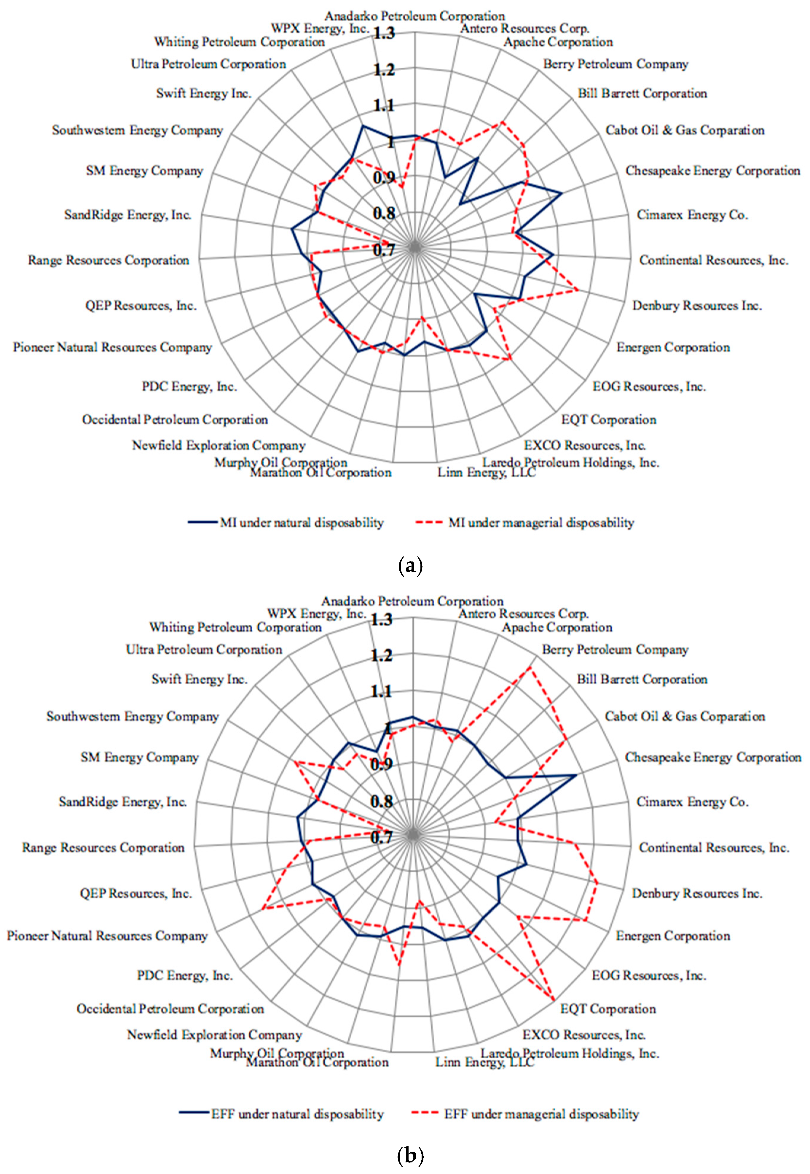
Figure 4 depicts the average MI, EFF and TECH indexes over 2011–2015 under natural and managerial disposability for the 31 oil and natural gas producers. We use the geometric mean to calculate the average, because MI, EFF and TECH are all multiplicative by nature [41]. The comparison between Figure 4 and Table 2, Table 3 and Table 4 provide several interesting findings with respect to MI. First, Figure 4 shows that the Malmquist indexes under managerial disposability exhibit significantly greater dispersions than the indexes under natural disposability. The indexes under managerial disposability can be as low as 0.715 for SandRidge Energy (Oklahoma City, OK, USA) and as high as 1.250 for EQT Corporation (Pittsburgh, PA, USA). The indexes from the natural disposability perspective are more restrained in variation, with the lowest being 0.950 of Marathon Oil (Houston, TX, USA) and the highest being 1.168 of Chesapeake Energy Corporation (Oklahoma City, OK, USA). The wild divergence of the Malmquist indexes under managerial disposability demonstrates that the producers have experienced very uneven growth in controlling carbon emissions through managerial efforts over 2011–2015. Second, 13 of the 31 producers exhibit a MI less than unity under natural disposability, and 19 producers have MI less than unity under managerial disposability. So there is a significant potential for these producers to improve their eco-productivity and catch up with the sustainability growth of other producers. Third, producers that have achieved full efficiency under natural disposability (i.e., Berry Petroleum Company (Denver, CO, USA), EOG Resources (Houston, TX, USA), Occidental Petroleum Corporation (Houston, TX, USA), and Swift Energy (Houston, TX, USA)) turn out to have MI close to unity. This indicates that there is little growth in their eco-productivity, plausibly because they have already performed well and further improvement is harder. Finally, Anadarko Petroleum Corporation (The Woodlands, TX, USA) and Chesapeake Energy Corporation (Oklahoma City, OK, USA), while having achieved perfect efficiency in UEM in every single year, actually exhibit Malmquist indexes less than unity. So their eco-productivity growth is limited and managerial efforts should be taken to improve the situation.
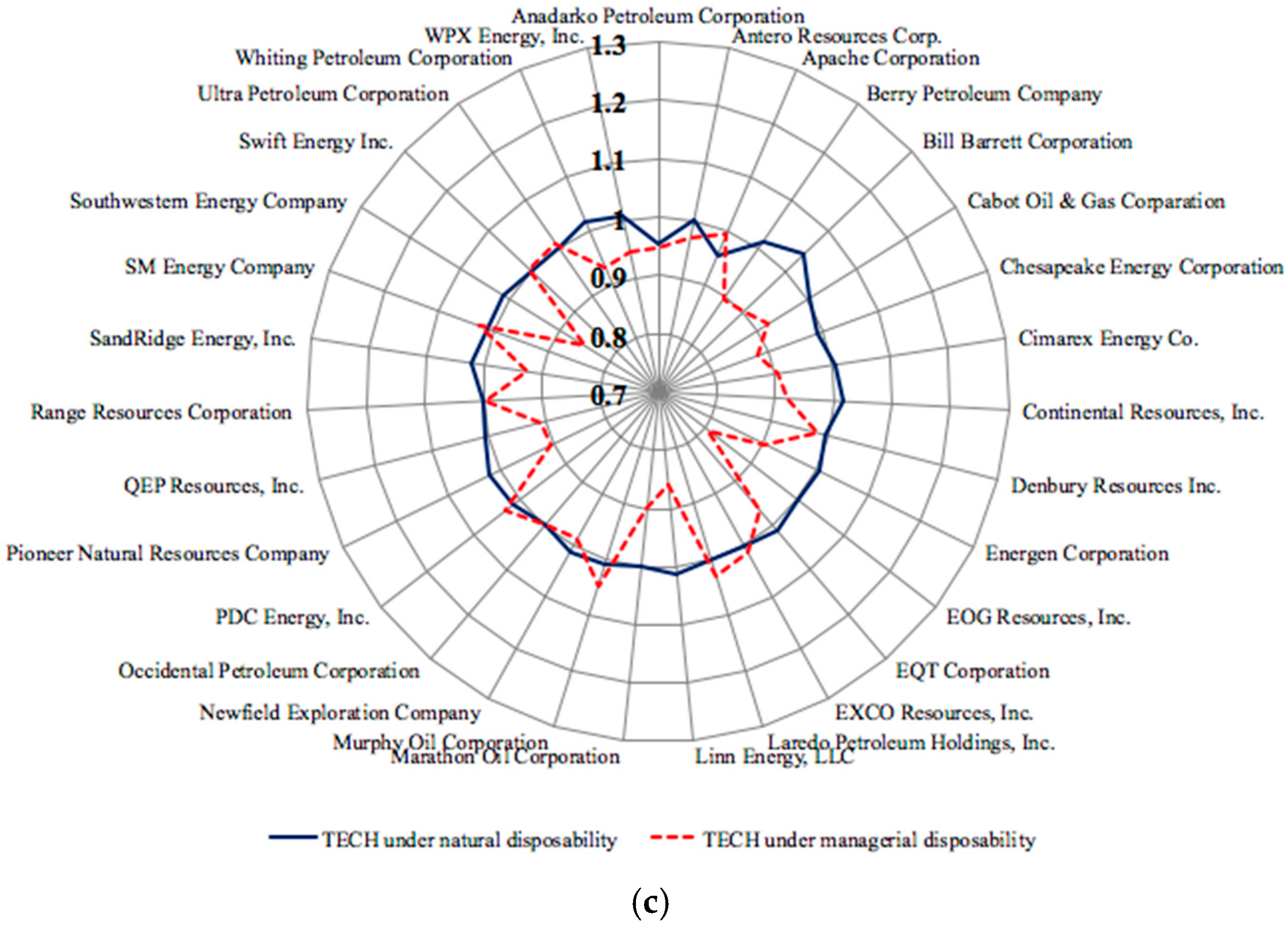
Figure 4 also shows interesting results about the EFF and TECH indexes. The EFF index measures how much closer a producer moves to the efficiency frontier over time. The TECH index measures the frontier shift caused by technical change. Panel (b) shows that under natural disposability, almost all producers have EFF close to one except Chesapeake Energy Corporation. The high EFF of Chesapeake indicates that the company has made significant progresses in catching up with efficient companies on the frontier. Meanwhile, its TECH is close to one. Hence, the company’s growth in eco-productivity is driven by its ability to catch up the frontier, rather than the industry-wide technical change. Under managerial disposability, the EFF indexes display wider variations. Panel (c) shows that under natural disposability, the TECH indexes stay close to one and remain relatively stable across the producers. However, under managerial disposability, most of the TECH indexes drop below unity, indicating an industry-wide loss of efficiency in terms of technical change. Among all the producers, EOG Resources (Houston, TX, USA), Linn Energy (Houston, TX, USA) and Southwestern Energy Company (Houston, TX, USA) have the worst TECH indexes.
5. Discussions and Conclusions
This study assesses the carbon emission performance of the US oil and natural gas independent producers by applying the DEA and Malmquist index measurement methodology under natural disposability and managerial disposability respectively. The assessment takes the drilling activity and carbon emissions into account, along with other operational and financial factors. We find that on average, the Malmquist index under natural disposability has improved from 2012 to 2015. The variations of Malmquist indexes across the independent producers under natural disposability are significantly smaller than those under managerial disposability. That is, the independent producers show relatively uniform changes in eco-productivity under natural disposability, while under managerial disposability the changes are quite unbalanced among the producers. By decomposing the Malmquist index into efficiency change and technical change, we can pinpoint the driving force behind the change of eco-productivity. We find that under natural disposability, the efficiency change indexes are quite stable and close to unity. But under managerial disposability there is an industry-wide efficiency loss in technical change in 2011–2015.
The aforementioned results bear the following implications for the oil and gas industry as well as the policymakers. First, the large variations of Malmquist indexes under managerial disposability imply that company managers should strive to ensure more consistent performance by imposing more uniform management practices on carbon emissions, so the industry can act in a more synchronized way. While there is a solid consensus among the companies that climate change is an important problem that should be dealt with by the oil and gas industry, what specific actions should be taken by the companies remains a highly contentious issue. Policymakers may consider to provide guidelines or even regulations to govern the industry practices.
However, the US political environment may not be supportive in the near term. On 1 June 2017, the newly elected President Trump announced that US would withdraw from the Paris Agreement, citing economic reasons [45]. Preliminary analysis shows that the US is unlikely to achieve its 2025 goal promised under the agreement [46]. The unfavorable political environment makes it very likely that the efficiency loss in tackling carbon emissions under managerial disposability in 2011–2015 will become even worse in the near future. Given the political environment, the voluntary mitigation actions from oil and gas producers may need to play a larger role in the near future. From the economics perspective, the “first-best” solution to climate change problem is to impose a uniform price on carbon emissions through policy instruments like carbon tax. In this first-best solution, voluntary actions by firms would not be needed. In reality, the feasibility of the first-best solution is severely undermined by many real-world complications. There is a growing argument among policymakers and researchers that firms, through voluntary actions, may play a more proactive and significant role in tackling climate change. Various voluntary environmental management certification programs (e.g., ISO 14001) have been set up to promote and guide environmental actions for firms. To tackle the climate change problem, independent oil and gas producers may consult these voluntary certification programs.
Several emission mitigation measures are readily available for the producers to improve their carbon emission performance, including energy conservation, leak detection and repair, and flaring reduction. Usually the mitigation measures, if done properly, can also bring economic benefits. For example, energy conservation through more efficient field operations can reduce energy cost. Through flaring reduction technology, gas that would otherwise be flared can be captured and used for other purposes. Furthermore, a potential but more radical action that can be taken by independent oil and gas producers is to invest in renewable energy, to offset the carbon footprints they generate in the production process. Indeed, some integrated oil and gas companies have noticed the importance of renewable energy and ventured into the field. For instance, Chevron (San Ramon, CA, USA) and BP (London, UK) have set up their renewable departments to invest in solar. BP first entered the solar energy industry in 1980s through acquisition of an existing solar module manufacturer. The company branched into the installation business in California in 2000s. But in 2011 BP shut down its solar business including manufacturing and installation. Chevron followed the footsteps of BP to close its solar energy business in 2014. The downfall of the solar business at BP and Chevron seems to validate the argument raised by existing research that oil companies are prone to regard renewable energy as a public relation vehicle rather than a sustainable core business asset [47]. This is a lesson that should be learned by the independent oil and gas producers. The transition to renewable energy is a vital step for climate change mitigation. On the supply side, falling costs make renewable energy especially wind and solar increasingly competitive. On the demand side, the shift to electric vehicles is accelerating. Recently, several countries (China, United Kingdom, France, Norway, etc.) have announced their intentions to ban fossil-fuel vehicles and the number of such countries is on the rise [48]. The transition to cleaner vehicles is very bearish for the oil and gas industry. The producers may need to reconsider their business models in face of the shift to renewable energy before it is too late.
The study has the following limitations. First, due to lack of data, the current study is unable to cover all the independent producers. The volume of emissions under study accounts for around 50% of the total emissions from the independent producers. Different producers have different operating strategies and assets. It would be interesting to investigate other producers once data are available. Second, since the companies’ annual reports typically provide the total production without separating it into onshore and offshore production, the study does not distinguish between onshore and offshore production. Therefore, what the study yields is the aggregate performance of the producers. Once detailed data for onshore and offshore production are available, we will be able to benchmark onshore and offshore production separately.
This study suggests two avenues for future research. First, the carbon emission performance of an oil and gas producer is affected by many factors, such as the producer’s perception of climate risk, the stakeholder pressures, and technology choice [49,50]. Understanding the factors behind the carbon emission performance can help with designing policy instruments to enhance the sustainable development of the industry. Second, it is possible to extend the study of carbon emission performance beyond the upstream production sector to other stages in the oil and gas value chain, such as refining, transportation and distribution.
Supplementary Materials
Please refer to the attached sample data used in this research. The following are available online at www.mdpi.com/2071-1050/10/1/110/s1.
Acknowledgments
This work is supported by research program at China University of Political Science and Law.
Author Contributions
Tianchi Li collected and organized the data, and performed part of the computation; Derek Wang conceived the conceptual framework of the study, developed the methodology, performed part of the computation, and wrote the paper.
Conflicts of Interest
The authors declare no conflict of interest.
References
- Van den Hove, S.; Le Menestrel, M.; de Bettignies, H.-C. The oil industry and climate change: Strategies and ethical dilemmas. Clim. Policy 2002, 2, 3–18. [Google Scholar] [CrossRef]
- Skjaerseth, J.B.; Skodvin, T. Climate Change and the Oil Industry: Common Problems, Different Strategies. Glob. Environ. Politics 2001, 1, 43–64. [Google Scholar] [CrossRef]
- Hiatt, S.R.; Grandy, J.B.; Lee, B.H. Organizational Responses to Public and Private Politics: An Analysis of Climate Change Activists and U.S. Oil and Gas Firms. Organ. Sci. 2015, 26, 1769–1786. [Google Scholar] [CrossRef]
- Weitz, M. U.S. EPA GHG Emission Data: Natural Gas and Petroleum Systems. Available online: https://www.epa.gov/sites/production/files/2015-09/documents/weitz_pres.pdf (accessed on 10 December 2017).
- EPA. Greenhouse Gas Emissions Reporting From the Petroleum and Natural Gas Industry. Available online: https://www.epa.gov/ghgreporting/greenhouse-gas-emissions-reporting-petroleum-and-natural-gas-industry-background (accessed on 10 December 2017).
- Weinhold, B. The Future of Fracking: New Rules Target Air Emissions for Cleaner Natural Gas Production. Environ. Health Perspect. 2012, 120, a272–a279. [Google Scholar] [CrossRef] [PubMed]
- Dittrick, P. EPA’s Deadline on Drilling-Related Air Pollution Standards Extended. Available online: http://www.ogj.com/articles/2012/04/epas-deadline-on-drilling-related-air-pollution-standards-extended.html (accessed on 30 December 2017).
- Sueyoshi, T.; Goto, M. Weak and strong disposability vs. natural and managerial disposability in DEA environmental assessment: Comparison between Japanese electric power industry and manufacturing industries. Energy Econ. 2012, 34, 686–699. [Google Scholar] [CrossRef]
- Levy, D.L.; Kolk, A. Strategic Responses to Global Climate Change: Conflicting Pressures on Multinationals in the Oil Industry. Bus. Politics 2002, 4, 275–300. [Google Scholar] [CrossRef]
- Kolk, A.; Levy, D. Winds of Change: Corporate Strategy, Climate change and Oil Multinationals. Eur. Manag. J. 2001, 19, 501–509. [Google Scholar] [CrossRef]
- Silvestre, B.S.; Gimenes, F.A.P.; Neto, R.S. A sustainability paradox? Sustainable operations in the offshore oil and gas industry: The case of Petrobras. J. Clean. Prod. 2017, 142, 360–370. [Google Scholar] [CrossRef]
- Nasiritousi, N. Fossil fuel emitters and climate change: Unpacking the governance activities of large oil and gas companies. Environ. Politics 2017, 26, 621–647. [Google Scholar] [CrossRef]
- Jung, E.; Kim, J.; Rhee, S. The measurement of corporate environmental performance and its application to the analysis of efficiency in oil industry. J. Clean. Prod. 2001, 9, 551–563. [Google Scholar] [CrossRef]
- Paun, D. Sustainability and Financial Performance of Companies in the Energy Sector in Romania. Sustainability 2017, 9, 1722. [Google Scholar] [CrossRef]
- Shvarts, E.A.; Pakhalov, A.M.; Knizhnikov, A.Y. Assessment of environmental responsibility of oil and gas companies in Russia: The rating method. J. Clean. Prod. 2016, 127, 143–151. [Google Scholar] [CrossRef]
- Alazzani, A.; Wan-Hussin, W.N. Global Reporting Initiative’s environmental reporting: A study of oil and gas companies. Ecol. Indic. 2013, 32, 19–24. [Google Scholar] [CrossRef]
- Wang, D.; Li, S.; Sueyoshi, T. DEA environmental assessment on U.S. industrial sectors: Investment for improvement in operational and environmental performance to attain corporate sustainability. Energy Econ. 2014, 45, 254–267. [Google Scholar] [CrossRef]
- Zhao, X.; Zhong, C. Low Carbon Economy Performance Analysis with the Intertemporal Effect of Capital in China. Sustainability 2017, 9, 853. [Google Scholar]
- Cao, L.; Qi, Z.; Ren, J. China’s Industrial Total-Factor Energy Productivity Growth at Sub-Industry Level: A Two-Step Stochastic Metafrontier Malmquist Index Approach. Sustainability 2017, 9, 1384. [Google Scholar]
- Meng, M.; Fu, Y.; Wang, T.; Jing, K. Analysis of Low-Carbon Economy Efficiency of Chinese Industrial Sectors Based on a RAM Model with Undesirable Outputs. Sustainability 2017, 9, 451. [Google Scholar] [CrossRef]
- Klumpp, M. Do Forwarders Improve Sustainability Efficiency? Evidence from a European DEA Malmquist Index Calculation. Sustainability 2017, 9, 842. [Google Scholar] [CrossRef]
- Gómez-Calvet, R.; Conesa, D.; Gómez-Calvet, A.R.; Tortosa-Ausina, E. Energy efficiency in the European Union: What can be learned from the joint application of directional distance functions and slacks-based measures? Appl. Energy 2014, 132, 137–154. [Google Scholar] [CrossRef]
- Wang, D.D.; Sueyoshi, T. Assessment of large commercial rooftop photovoltaic system installations: Evidence from California. Appl. Energy 2017, 188, 45–55. [Google Scholar] [CrossRef]
- Sueyoshi, T.; Wang, D. Measuring scale efficiency and returns to scale on large commercial rooftop photovoltaic systems in California. Energy Econ. 2017, 65, 389–398. [Google Scholar] [CrossRef]
- Wang, D.D. Do United States manufacturing companies benefit from climate change mitigation technologies? J. Clean. Prod. 2017, 161, 821–830. [Google Scholar] [CrossRef]
- Sueyoshi, T.; Yuan, Y.; Goto, M. A literature study for DEA applied to energy and environment. Energy Econ. 2017, 62, 104–124. [Google Scholar] [CrossRef]
- Li, J.; Li, J.; Zheng, F. Unified Efficiency Measurement of Electric Power Supply Companies in China. Sustainability 2014, 6, 779–793. [Google Scholar] [CrossRef]
- Sueyoshi, T.; Goto, M. Data envelopment analysis for environmental assessment: Comparison between public and private ownership in petroleum industry. Eur. J. Oper. Res. 2012, 216, 668–678. [Google Scholar] [CrossRef]
- Sueyoshi, T.; Goto, M. DEA environmental assessment in time horizon: Radial approach for Malmquist index measurement on petroleum companies. Energy Econ. 2015, 51, 329–345. [Google Scholar] [CrossRef]
- Sueyoshi, T.; Wang, D. Sustainability development for supply chain management in U.S. petroleum industry by DEA environmental assessment. Energy Econ. 2014, 46, 306–374. [Google Scholar] [CrossRef]
- Bevilacqua, M.; Braglia, M. Environmental efficiency analysis for ENI oil refineries. J. Clean. Prod. 2002, 10, 85–92. [Google Scholar] [CrossRef]
- Malmquist, S. Index numbers and indifference surfaces. Trab. Estad. 1953, 4, 209–242. [Google Scholar] [CrossRef]
- Bjurek, H.; Hjalmarsson, L. Productivity in multiple output public service: A quadratic frontier function and Malmquist index approach. J. Public Econ. 1995, 56, 447–460. [Google Scholar] [CrossRef]
- Grifell-Tatjé, E.; Lovell, C.A.K. A note on the Malmquist productivity index. Econ. Lett. 1995, 47, 169–175. [Google Scholar] [CrossRef]
- Färe, R.; Grosskopf, S.; Lindgren, B.; Roos, P. Productivity Developments in Swedish Hospitals: A Malmquist Output Index Approach. In Data Envelopment Analysis: Theory, Methodology, and Applications; Springer: Dordrecht, The Netherlands, 1994; pp. 253–272. [Google Scholar]
- Mahlberg, B.; Luptacik, M. Eco-efficiency and eco-productivity change over time in a multisectoral economic system. Eur. J. Oper. Res. 2014, 234, 885–897. [Google Scholar] [CrossRef]
- Asmild, M.; Paradi, J.C.; Aggarwall, V.; Schaffnit, C. Combining DEA Window Analysis with the Malmquist Index Approach in a Study of the Canadian Banking Industry. J. Product. Anal. 2004, 21, 67–89. [Google Scholar] [CrossRef]
- Chung, Y.H.; Färe, R.; Grosskopf, S. Productivity and Undesirable Outputs: A Directional Distance Function Approach. J. Environ. Manag. 1997, 51, 229–240. [Google Scholar] [CrossRef]
- Lovell, C.A.K. The Decomposition of Malmquist Productivity Indexes. J. Product. Anal. 2003, 20, 437–458. [Google Scholar] [CrossRef]
- Fare, R.; Grosskopf, S.; Pasurka, C.A., Jr. Accounting for Air Pollution Emissions in Measures of State Manufacturing Productivity Growth. J. Reg. Sci. 2001, 41, 381–409. [Google Scholar] [CrossRef]
- Färe, R.; Grosskopf, S.; Norris, M.; Zhang, Z. Productivity Growth, Technical Progress, and Efficiency Change in Industrialized Countries. Am. Econ. Rev. 1994, 84, 66–83. [Google Scholar]
- Charnes, A.; Cooper, W.W.; Rhodes, E. Measuring the efficiency of decision making units. Eur. J. Oper. Res. 1978, 2, 429–444. [Google Scholar] [CrossRef]
- Dakpo, K.H.; Jeanneaux, P.; Latruffe, L. Modelling pollution-generating technologies in performance benchmarking: Recent developments, limits and future prospects in the nonparametric framework. Eur. J. Oper. Res. 2016, 250, 347–359. [Google Scholar] [CrossRef]
- Raab, R.; Lichty, R. Identifying subareas that comprise a greater metropolitan area: The criterion of county relative efficiency. J. Reg. Sci. 2002, 42, 579–594. [Google Scholar] [CrossRef]
- The White House. Statement by President Trump on the Paris Climate Accord. Available online: https://www.whitehouse.gov/the-press-office/2017/06/01/statement-president-trump-paris-climate-accord (accessed on 10 August 2017).
- Cornwall, W. Can U.S. states and cities overcome Paris exit? Science 2017, 356, 764. [Google Scholar] [CrossRef] [PubMed]
- Miller, D. Why the oil companies lost solar. Energy Policy 2013, 60, 52–60. [Google Scholar] [CrossRef]
- CNN. These Countries Want to Ban Gas and Diesel Cars. Available online: http://money.cnn.com/2017/09/11/autos/countries-banning-diesel-gas-cars/index.html (accessed on 30 December 2017).
- Sprengel, D.; Busch, T. Stakeholder engagement and environmental strategy—The case of climate change. Bus. Strategy Environ. 2011, 20, 351–364. [Google Scholar] [CrossRef]
- Wang, D. Unraveling the Effects of Environmental Technology Portfolio on Corporate Sustainable Development. Corp. Soc. Responsib. Environ. Manag. 2017, in press. [Google Scholar]
Figure 1.
Total carbon emissions from onshore and offshore production for 2011–2015, by production sites and producers.
Figure 1.
Total carbon emissions from onshore and offshore production for 2011–2015, by production sites and producers.
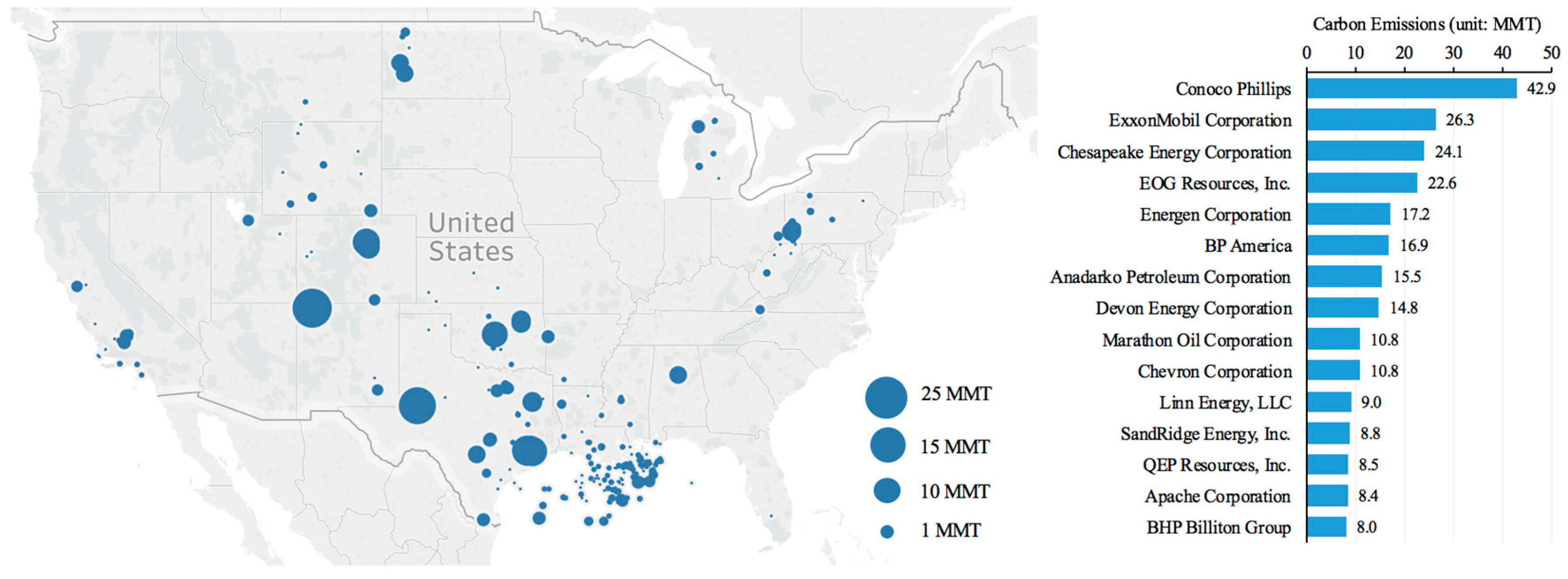
Figure 2.
Annual carbon emissions from integrated and independent producers, 2011–2015.
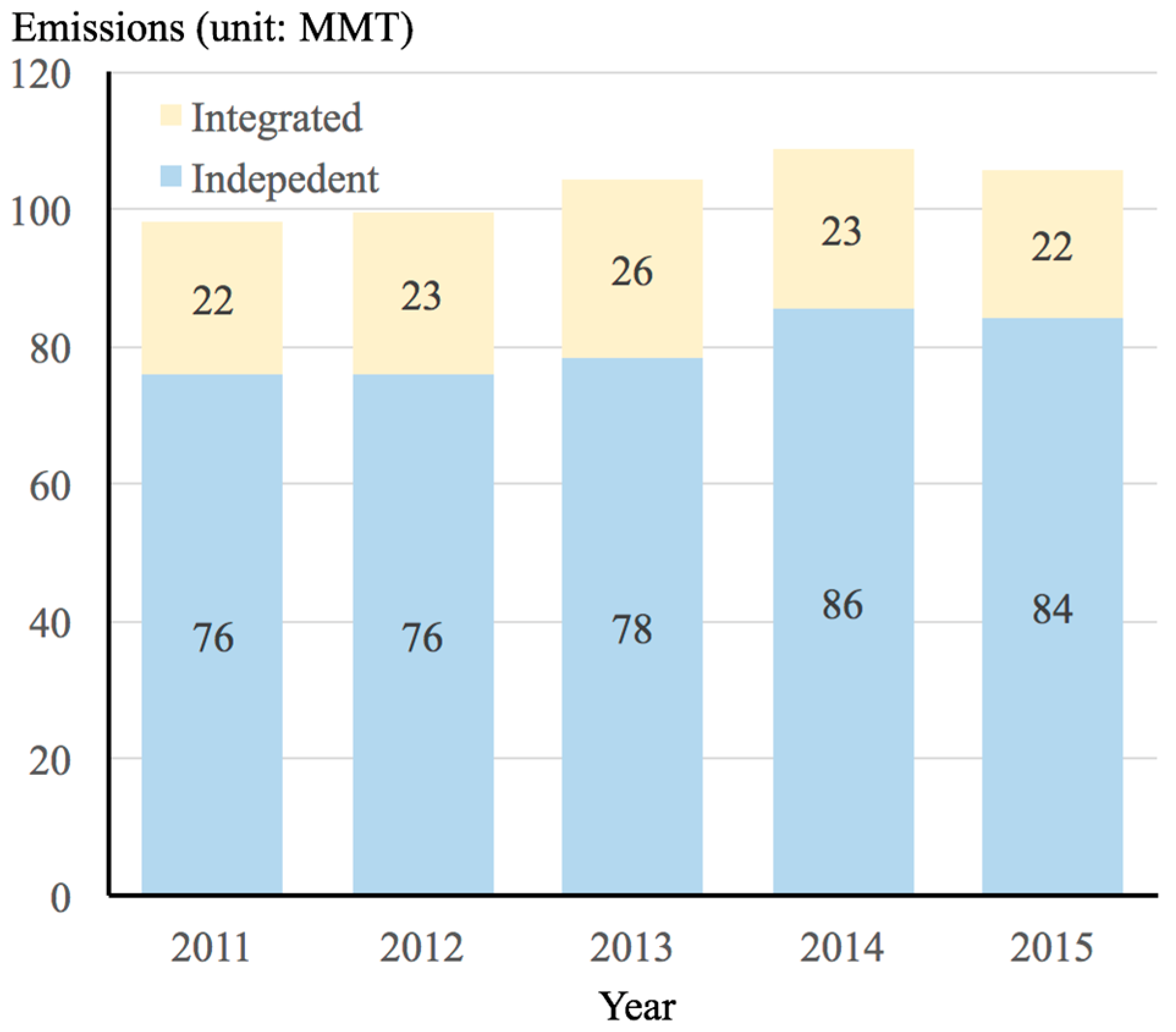
Figure 3.
Distribution of the Malmquist indexes per year, 2012–2015. (a) Natural disposability; (b) Managerial disposability.
Figure 3.
Distribution of the Malmquist indexes per year, 2012–2015. (a) Natural disposability; (b) Managerial disposability.
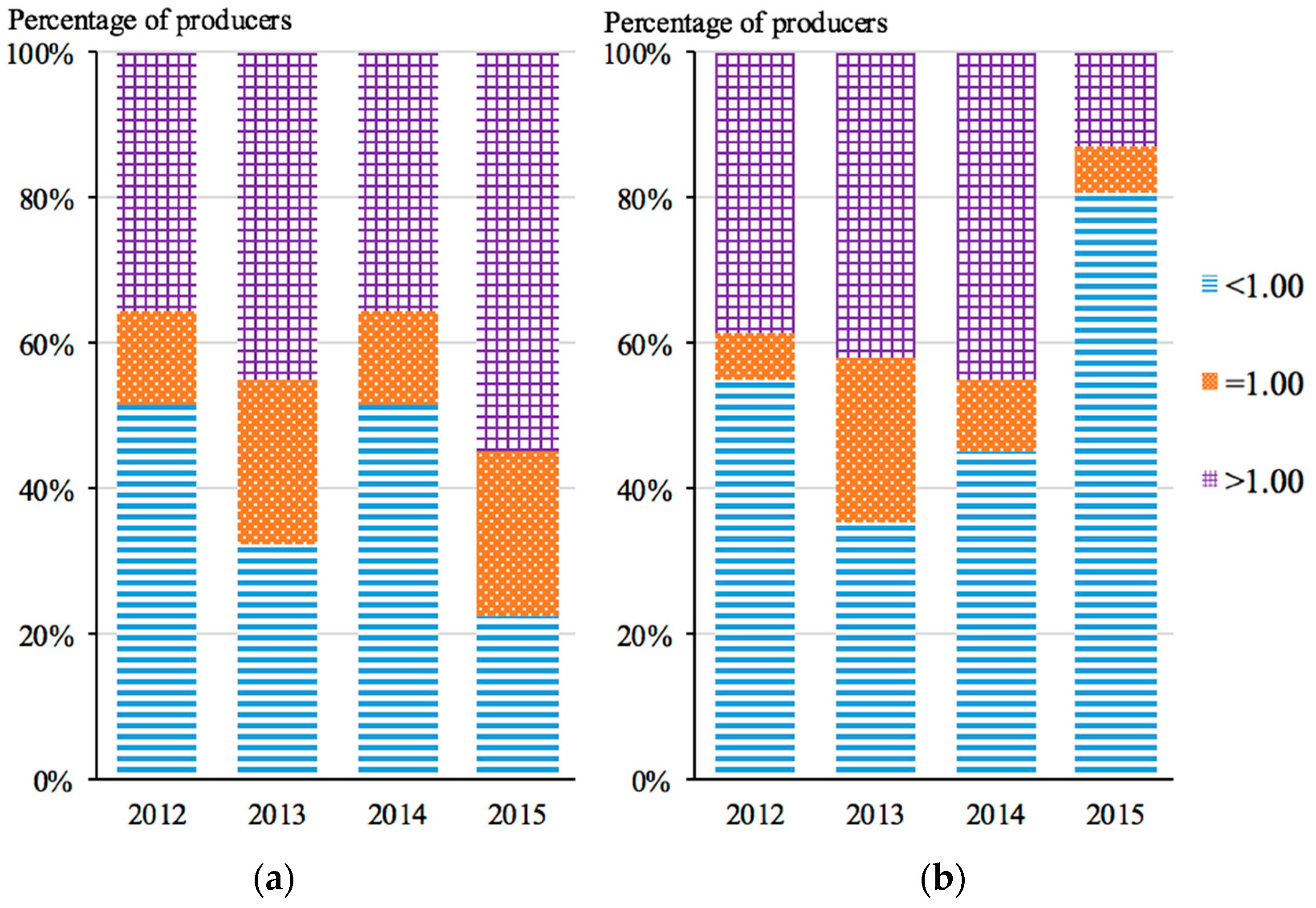
Figure 4.
Average MI, EFF and TECH indexes under natural disposability and managerial disposability for oil and natural gas producers during 2011–2015. (a) Average MI for the producers during 2011–2015; (b) Average EFF for the producers during 2011–2015; (c) Average TECH for the producers during 2011–2015.

Table 1.
Summary statistics of inputs and outputs, 2011–2015.
| Total Assets | Operational Expense | Wells Drilled | Oil Production | Natural Gas Production | Revenue | GHG Emissions | |
|---|---|---|---|---|---|---|---|
| Unit: | Million $ | Million $ | No. | MBbls/Day | MMcf/Day | Million $ | Thousand Tons |
| 2011 | |||||||
| Mean | 13,384 | 2701 | 363 | 69.17 | 714.09 | 4307 | 1340 |
| Std. dev. | 16,309 | 3698 | 364 | 187.56 | 1394.04 | 5924 | 1254 |
| Min | 1615 | 160 | 24 | 0.01 | 0.48 | 337 | 149 |
| Max | 60,044 | 15,837 | 1282 | 1043.31 | 7327.46 | 24,119 | 4824 |
| 2012 | |||||||
| Mean | 14,578 | 3217 | 349 | 82.94 | 753.82 | 4458 | 1330 |
| Std. dev. | 17,561 | 3748 | 330 | 211.36 | 1351.41 | 6044 | 1179 |
| Min | 1992 | 283 | 41 | 0.01 | 0.39 | 321 | 161 |
| Max | 64,210 | 14,010 | 1272 | 1178.10 | 6934.35 | 24,253 | 4439 |
| 2013 | |||||||
| Mean | 15,607 | 3344 | 320 | 96.69 | 744.66 | 4973 | 1328 |
| Std. dev. | 18,243 | 3941 | 277 | 238.89 | 1219.73 | 6460 | 1260 |
| Min | 2331 | 401 | 45 | 0.01 | 0.32 | 411 | 123 |
| Max | 69,443 | 15,437 | 985 | 1333.80 | 6020.49 | 25,736 | 5279 |
| 2014 | |||||||
| Mean | 16,312 | 3903 | 353 | 89.93 | 742.01 | 5438 | 1430 |
| Std. dev. | 16,768 | 5140 | 244 | 171.74 | 1116.87 | 6501 | 1391 |
| Min | 2173 | 567 | 30 | 0.01 | 0.63 | 472 | 63 |
| Max | 60,967 | 19,648 | 869 | 937.27 | 5222.85 | 23,125 | 5578 |
| 2015 | |||||||
| Mean | 11,507 | 5913 | 217 | 96.16 | 740.32 | 3156 | 1321 |
| Std. dev. | 11,612 | 6735 | 141 | 177.12 | 1038.01 | 3414 | 1223 |
| Min | 525 | 659 | 15 | 0.01 | 0.74 | 208 | 67 |
| Max | 46,414 | 31,683 | 603 | 964.61 | 4572.25 | 12,764 | 4580 |
MBbls stands for thousand barrels; MMcf stands for million cubic feet.
Table 2.
Unified efficiency under natural disposability.
| Company | 2011 | 2012 | 2013 | 2014 | 2015 | 2011–2015 |
|---|---|---|---|---|---|---|
| Pioneer Natural Resources Company | 1.000 | 1.000 | 1.000 | 1.000 | 1.000 | 1.000 |
| Laredo Petroleum Holdings, Inc. | 1.000 | 1.000 | 1.000 | 1.000 | 1.000 | 1.000 |
| Swift Energy Inc. | 1.000 | 1.000 | 1.000 | 1.000 | 1.000 | 1.000 |
| PDC Energy, Inc. | 1.000 | 1.000 | 1.000 | 1.000 | 1.000 | 1.000 |
| Occidental Petroleum Corporation | 1.000 | 1.000 | 1.000 | 1.000 | 1.000 | 1.000 |
| Ultra Petroleum Corporation | 0.969 | 1.000 | 1.000 | 1.000 | 1.000 | 0.994 |
| Bill Barrett Corporation | 0.961 | 1.000 | 1.000 | 1.000 | 1.000 | 0.992 |
| EXCO Resources, Inc. | 0.953 | 1.000 | 1.000 | 1.000 | 1.000 | 0.991 |
| Range Resources Corporation | 0.951 | 1.000 | 1.000 | 1.000 | 1.000 | 0.990 |
| Denbury Resources Inc. | 0.938 | 1.000 | 1.000 | 1.000 | 1.000 | 0.988 |
| Antero Resources Corp. | 1.000 | 1.000 | 0.964 | 0.960 | 1.000 | 0.985 |
| SM Energy Company | 1.000 | 1.000 | 1.000 | 0.961 | 0.933 | 0.979 |
| Cabot Oil & Gas Corporation | 0.943 | 0.939 | 1.000 | 1.000 | 1.000 | 0.976 |
| Murphy Oil Corporation | 1.000 | 1.000 | 0.942 | 1.000 | 0.939 | 0.976 |
| Berry Petroleum Company | 0.954 | 1.000 | 0.903 | 1.000 | 1.000 | 0.971 |
| Southwestern Energy Company | 0.963 | 1.000 | 1.000 | 0.822 | 1.000 | 0.957 |
| Marathon Oil Corporation | 1.000 | 1.000 | 1.000 | 0.953 | 0.755 | 0.942 |
| Cimarex Energy Co. | 0.957 | 0.932 | 0.930 | 0.913 | 0.887 | 0.924 |
| EQT Corporation | 0.886 | 0.966 | 0.921 | 0.921 | 0.920 | 0.923 |
| Whiting Petroleum Corporation | 0.969 | 0.851 | 0.907 | 0.850 | 1.000 | 0.915 |
| WPX Energy, Inc. | 0.894 | 0.887 | 0.842 | 0.925 | 1.000 | 0.910 |
| Newfield Exploration Company | 0.864 | 0.890 | 0.902 | 0.869 | 1.000 | 0.905 |
| Energen Corporation | 1.000 | 1.000 | 0.766 | 0.884 | 0.857 | 0.901 |
| Linn Energy, LLC | 0.941 | 1.000 | 0.835 | 0.669 | 0.931 | 0.875 |
| SandRidge Energy, Inc. | 0.829 | 0.925 | 0.838 | 0.866 | 0.891 | 0.870 |
| Continental Resources, Inc. | 0.890 | 0.874 | 0.887 | 0.844 | 0.828 | 0.865 |
| EOG Resources, Inc. | 0.807 | 0.786 | 1.000 | 1.000 | 0.724 | 0.863 |
| Chesapeake Energy Corporation | 0.635 | 0.582 | 1.000 | 1.000 | 1.000 | 0.843 |
| QEP Resources, Inc. | 0.730 | 0.913 | 0.754 | 0.924 | 0.873 | 0.839 |
| Anadarko Petroleum Corporation | 0.625 | 1.000 | 0.691 | 0.846 | 0.710 | 0.774 |
| Apache Corporation | 0.460 | 0.741 | 0.691 | 0.638 | 0.773 | 0.661 |
Table 3.
Unified efficiency under managerial disposability.
| Company | 2011 | 2012 | 2013 | 2014 | 2015 | 2011–2015 |
|---|---|---|---|---|---|---|
| Occidental Petroleum Corporation | 1.000 | 1.000 | 1.000 | 1.000 | 1.000 | 1.000 |
| Anadarko Petroleum Corporation | 1.000 | 1.000 | 1.000 | 1.000 | 1.000 | 1.000 |
| Pioneer Natural Resources Company | 1.000 | 1.000 | 1.000 | 1.000 | 1.000 | 1.000 |
| Chesapeake Energy Corporation | 1.000 | 1.000 | 1.000 | 1.000 | 1.000 | 1.000 |
| Apache Corporation | 0.894 | 1.000 | 1.000 | 1.000 | 1.000 | 0.979 |
| Range Resources Corporation | 0.960 | 1.000 | 1.000 | 1.000 | 0.880 | 0.968 |
| Laredo Petroleum Holdings, Inc. | 1.000 | 0.949 | 1.000 | 0.862 | 0.869 | 0.936 |
| Ultra Petroleum Corporation | 0.890 | 1.000 | 0.907 | 0.832 | 0.794 | 0.885 |
| Denbury Resources Inc. | 0.592 | 1.000 | 0.935 | 0.859 | 1.000 | 0.877 |
| Swift Energy Inc. | 0.916 | 0.943 | 0.882 | 0.847 | 0.782 | 0.874 |
| EOG Resources, Inc. | 0.771 | 0.818 | 0.856 | 1.000 | 0.812 | 0.852 |
| Marathon Oil Corporation | 1.000 | 0.842 | 0.827 | 0.764 | 0.744 | 0.836 |
| Murphy Oil Corporation | 1.000 | 0.861 | 0.663 | 0.697 | 0.904 | 0.825 |
| EQT Corporation | 0.569 | 0.934 | 0.767 | 0.902 | 0.830 | 0.800 |
| Antero Resources Corp. | 0.862 | 0.660 | 0.781 | 0.807 | 0.848 | 0.792 |
| Bill Barrett Corporation | 0.665 | 0.599 | 0.739 | 0.884 | 1.000 | 0.777 |
| EXCO Resources, Inc. | 0.783 | 0.800 | 0.740 | 0.792 | 0.759 | 0.775 |
| Berry Petroleum Company | 0.655 | 0.618 | 0.591 | 1.000 | 1.000 | 0.773 |
| WPX Energy, Inc. | 1.000 | 0.674 | 0.671 | 0.629 | 0.582 | 0.711 |
| Cabot Oil & Gas Corparation | 0.595 | 0.595 | 0.800 | 0.860 | 0.689 | 0.708 |
| SandRidge Energy, Inc. | 1.000 | 0.652 | 0.658 | 0.605 | 0.545 | 0.692 |
| Whiting Petroleum Corporation | 0.823 | 0.773 | 0.654 | 0.574 | 0.605 | 0.686 |
| PDC Energy, Inc. | 0.773 | 0.647 | 0.689 | 0.689 | 0.625 | 0.685 |
| Southwestern Energy Company | 0.655 | 0.674 | 0.668 | 0.694 | 0.718 | 0.682 |
| SM Energy Company | 0.766 | 0.660 | 0.691 | 0.673 | 0.614 | 0.681 |
| Newfield Exploration Company | 0.662 | 0.747 | 0.735 | 0.635 | 0.604 | 0.676 |
| Linn Energy, LLC | 0.796 | 0.640 | 0.668 | 0.645 | 0.578 | 0.665 |
| Continental Resources, Inc. | 0.559 | 0.646 | 0.663 | 0.664 | 0.651 | 0.637 |
| QEP Resources, Inc. | 0.615 | 0.629 | 0.618 | 0.585 | 0.580 | 0.605 |
| Cimarex Energy Co. | 0.687 | 0.610 | 0.596 | 0.559 | 0.558 | 0.602 |
| Energen Corporation | 0.440 | 0.520 | 0.537 | 0.452 | 0.476 | 0.485 |
Table 4.
MI, EFF and TECH indexes under natural disposability and managerial disposability.
| UEN | UEM | ||||||
|---|---|---|---|---|---|---|---|
| MI | EFF | TECH | MI | EFF | TECH | ||
| 2011–2012 | Mean | 0.985 | 1.025 | 0.972 | 1.022 | 1.005 | 1.021 |
| Std. dev. | 0.118 | 0.120 | 0.089 | 0.203 | 0.219 | 0.058 | |
| Min | 0.559 | 0.893 | 0.537 | 0.635 | 0.652 | 0.931 | |
| Max | 1.344 | 1.601 | 1.058 | 1.647 | 1.689 | 1.215 | |
| 2012–2013 | Mean | 1.007 | 1.006 | 1.009 | 0.999 | 1.003 | 0.997 |
| Std. dev. | 0.165 | 0.159 | 0.044 | 0.111 | 0.109 | 0.038 | |
| Min | 0.833 | 0.691 | 0.921 | 0.799 | 0.771 | 0.806 | |
| Max | 1.711 | 1.717 | 1.206 | 1.349 | 1.345 | 1.037 | |
| 2013–2014 | Mean | 1.003 | 1.006 | 1.001 | 1.045 | 1.011 | 1.035 |
| Std. dev. | 0.063 | 0.081 | 0.009 | 0.154 | 0.153 | 0.040 | |
| Min | 0.832 | 0.801 | 0.970 | 0.876 | 0.841 | 0.925 | |
| Max | 1.188 | 1.225 | 1.020 | 1.746 | 1.691 | 1.156 | |
| 2014–2015 | Mean | 1.007 | 1.007 | 1.008 | 0.980 | 0.983 | 0.997 |
| Std. dev. | 0.081 | 0.094 | 0.043 | 0.127 | 0.097 | 0.087 | |
| Min | 0.710 | 0.724 | 0.805 | 0.699 | 0.801 | 0.780 | |
| Max | 1.198 | 1.217 | 1.026 | 1.375 | 1.296 | 1.195 |
© 2018 by the authors. Licensee MDPI, Basel, Switzerland. This article is an open access article distributed under the terms and conditions of the Creative Commons Attribution (CC BY) license (http://creativecommons.org/licenses/by/4.0/).
Share and Cite
MDPI and ACS Style
Wang, D.; Li, T. Carbon Emission Performance of Independent Oil and Natural Gas Producers in the United States. Sustainability 2018, 10, 110. https://doi.org/10.3390/su10010110
AMA Style
Wang D, Li T. Carbon Emission Performance of Independent Oil and Natural Gas Producers in the United States. Sustainability. 2018; 10(1):110. https://doi.org/10.3390/su10010110
Chicago/Turabian StyleWang, Derek, and Tianchi Li. 2018. "Carbon Emission Performance of Independent Oil and Natural Gas Producers in the United States" Sustainability 10, no. 1: 110. https://doi.org/10.3390/su10010110
Note that from the first issue of 2016, this journal uses article numbers instead of page numbers. See further details here.