Quantifying the Effects of Wood Moisture and Temperature Variation on Time-of-Flight Acoustic Velocity Measures within Standing Red Pine and Jack Pine Trees

Abstract

The relationship between the dynamic modulus of elasticity (m_e) of xylem tissue and acoustic velocity (v_d) has been established for a number of commercially-important coniferous species, including red pine (Pinus resinosa Ait.) and jack pine (Pinus banksiana Lamb.). However, v_d has been shown to vary systematically with xylem temperature (t_x) and moisture (m_x) for some species, and hence when the calibrated m_e–v_d relationships are used outside of the range of conditions under which they were parameterized, erroneous predictions may arise. Consequently, the objectives of this study were (1) to investigate the significance of t_x and m_x effects on v_d measurements within standing red pine and jack pine trees, and (2), given (1), to develop correction equations for standardizing v_d measurements to referenced t_x and m_x conditions if warranted. Analytically, based on a temporal replicated sampling design, 26 mature red pine and 36 semi-mature jack pine trees growing in managed plantations located within central Ontario, Canada (Kirkwood Forest, Great Lakes—St. Lawrence Forest Region), were continuously measured for v_d, t_x, and m_x during the spring-to-autumn seasonal periods in 2016 (red pine) and 2017 (jack pine). A total of 6 measurement events per species occurred at approximately 4–8 week intervals in which a total of 624 red pine and 864 jack pine cardinal-specific (north, east, south, and west) breast-height acoustic velocity, xylem temperature, and xylem moisture measurements were obtained: Yielding a total of 156 red pine and 216 jack pine mean tree-based values available for analysis. Over the sampling periods, (1) mean tree xylem temperatures ranged from a minimum of 3 °C to a maximum of 31 °C (mean = 19.2 °C) in red pine and from a minimum of 0 °C to a maximum of 27 °C (mean = 16.5 °C) in jack pine, and (2) mean tree xylem moistures ranged from a minimum 31% to a maximum of 45% (mean = 38.6%) in red pine and from a minimum 25% to a maximum of 50% (mean = 38.8%) in jack pine. Graphical examination of the moisture effect on the v_d and t_x relationship by tree and species revealed inversely proportional, linear-like trends at lower moisture levels and directly-proportional, linear-like trends at higher moisture levels where the effect was more evident for red pine than for jack pine. In order to describe this multivariate relationship, species-specific, two-level hierarchical, mixed-effects linear models inclusive of random and fixed effects were specified and subsequently parameterized. The first-level model described the tree-specific v_d–t_x relationship deploying a simple linear regression specification, whereas the second-level model expressed the first-level parameter estimates as a linear function of seasonal mean tree moisture. The resultant statistically-validated, parameterized regression models, for which 64% (red pine) and 90% (jack pine) of the v_d variation was explained, indicated that the v_d–t_x relationship varied systematically with seasonal mean moisture level in red pine but not so in jack pine. More precisely, in red pine, v_d declined with increasing t_x at lower moisture levels (<38%), but increased with increasing t_x at higher moisture levels (>38%). Conversely, although v_d declined with increasing t_x in jack pine, the relationship was unaffected by changes in seasonal mean tree moisture levels. Consequently, based on the final hierarchical model specifications, correction equations for adjusting observed v_d values to standardized temperature (20 °C) and moisture conditions (40% for red pine) were developed for each species. Across the range of temperatures (≈5 °C–30 °C) and mean moisture levels (≈30–45%) examined, these equations generated a mean absolute v_d adjustment of approximately 0.12 km/s for red pine and 0.04 km/s for jack pine. However, based on the corresponding relative magnitude of these adjustments which account for the narrow species-specific v_d sample ranges observed (0.80 and 0.85 km/s for red pine and jack pine, respectively), the standardization of v_d estimates could be of operational significance when acoustic sampling during periods in which xylem temperature and moisture levels approach the extremities of their spring-to-autumn seasonal ranges. Overall, the results of this empirical-based assessment, which confirmed the presence of temperature and moisture induced variation in acoustic velocity measures within standing red pine and jack pine trees, were largely in accordance with expectation. The subsequent provision of species-specific correction functions for adjusting observed v_d sample values to corresponding equivalents referenced to standardized temperature and moisture conditions could assist in mitigating the consequences of environmental variability when acoustic sampling.

1. Introduction

Red pine (Pinus resinosa Ait.) and jack pine (Pinus banksiana Lamb.) are intensely-managed and commercially-important species that occupy a wide range of sandy textured sites throughout the Great Lakes—St. Lawrence and Boreal Forest Regions of North America [1]. These species produce a broad array of economically important end-products such as appearance-based boards for interior flooring, exterior decking and wall paneling, dimensional lumber for residential home construction, utility poles for building electrical transmission grids, veneer for furniture manufacturing, pulp and paper products, and engineered wood composites [2]. In order to optimize end-product recovery given this range of end-products, in-forest, non-destructive forecasting tools could be of consequential utility in terms of pre-harvest identification of end-product potential and informing post-harvest segregation decision-making so that the extracted raw fiber is routed to the most appropriate conversion facility (e.g., pulp and paper mills, stud and randomized length sawmills, or pole processing yards). Among the array of non-destructive methodologies used to estimate commercially-relevant wood attributes (see [3] for a comprehensive overview), acoustic-based methods have gained considerable currency in forest segregation operations given their ability to readily estimate one of the principal fiber attributes underlying solid-wood end-product type and grade: The modulus of elasticity (sensu [4]). Commercially available time-of-flight acoustic velocity instruments, such as the Director ST300 developed by Fibre-gen Inc. of Christchurch, New Zealand (e.g., [5]), and the TreeSonic microsecond timer developed by Fakopp Enterprise, Ágfalva, Hungary (e.g., [6]), can efficiently provide dynamic-based wood stiffness estimates for standing trees without restoring to more expensive and logistically challenging destructive methods (e.g., core extraction followed by Silviscan analysis).

More specifically, the relationship between the dynamic modulus of elasticity (MOE denoted m_e in this study) of the xylem tissue within standing trees and acoustic velocity (v_d; dilatational stress wave) has been established for numerous coniferous species including red pine [7] and jack pine [8]. Although there are many possible uses of the m_e–v_d relationship in both forest management and research, it has principally been deployed in pre-harvest surveys of end-product potential, segregation decision-making, and silvicultural experimentation when destructive methods are prohibited. However, acoustic velocity is known to vary by a multitude of internal factors related to the heterogeneity of the wood structure (e.g., ring width (growth rate) variation, knot distribution), in addition to the physical properties of the wood, when measured. With respect to these latter sources of variation, xylem temperature and wood moisture levels have been identified as being among the most important (e.g., [9,10,11,12]). Consequently, when acoustic-attribute relationships are used outside of the range of temperature and moisture conditions under which they were parameterized, erroneous predictions and associated end-product forecasts may occur.

Although limited to a small number of species, standardization equations which attempt to account for temperature and moisture effects on acoustic velocity measurements, have been developed (e.g., Scot pine (Pinus sylvestris L.); radiata pine (Pinus radiata D. Don), Salzmann pine (Pinus nigra salzmanni (Dunal) Franco), and maritime pine (Pinus pinaster Ait.); [13]). These equations adjust observed v_d sample values to corresponding equivalents referenced to standardized temperature and moisture conditions. However, the majority of the correction equations developed to date have been parameterized using measurement values obtained from solid wood end-products (e.g., sawn boards [12,14]) rather than from standing trees. Nevertheless, these research efforts have contributed to a more in-depth understanding of the importance of this issue when acoustic sampling, in addition to providing computational solutions for specific species.

Operationally, the acoustic approach to predicting internal fiber attributes within standing trees is increasingly being employed in (1) operational pre-harvest, end-product surveys in order to increase segregation efficiency and profit margins (e.g., [15,16]), and (2) silvicultural experimentation where acoustic velocity is utilized as a surrogate response metric for inferring wood quality (e.g., fertilization [17] and tree improvement [18] studies). Consequently, failure to account for the effect of temperature and moisture variation on acoustic velocity estimates could potentially lead to erroneous end-product forecasts in forest operations or statistical inference when analyzing experimental and survey results. Thus, with respect to standing red pine and jack pine trees for which a suite of acoustic-based fiber prediction models have been developed ([7,8], respectively), the objectives of this study were (1) to investigate the significance of xylem temperature and moisture effects on acoustic velocity, and (2), given (1), to develop correction equations for adjusting acoustic velocity measurements to standardized conditions if required.

2. Materials and Methods

2.1. Data Acquisition: Study Sites, Tree Selection and Associated Measurements

Twenty-six 85 year-old red pine and thirty-six 48 year-old jack pine trees growing in plantations established on good quality sites (site indices of 22 m at 50 years for both species, as determined from site-specific, height-age functions (i.e., [19] for red pine and [20] for jack pine)) in the Kirkwood Forest, which falls within Forest Section L.10—Algoma of the Great Lakes—St. Lawrence Forest Region [1], were chosen for repeated temporal-based measurement of acoustic velocity (v_d; km/s), xylem temperature (t_x; °C), and xylem moisture (m_x; %). Procedurally, for each of the replicated sampling events during the 2016 (n = 6 for red pine) and 2017 (n = 6 for jack pine) spring-to-autumn seasonal period, the following measurements were taken on each sample tree: (1) Twice-replicated mean v_d measurements, which were generated from 8 consecutive individual v_d estimates obtained on each cardinal-specific (north, east, south, and west) circumferential face using the ST300 time-of-flight acoustic velocity tool (±0.01 km/s; Fibre-gen Inc., New Zealand); the transmitter (impact) and receiving probes were positioned at stem heights of approximately 0.5 m and 1.5 m, respectively; and (2) cardinal-specific, breast-height (1.3 m) xylem temperature t_x (±0.1 °C) and temperature-adjusted m_x (±0.1%) measurements at an xylem depth of approximately 3 cm from the periderm circumferential surface as determined using a Gann Hydromette M 4050 electrical-resistance, multi-functional meter equipped with a Gann M 18 Electrode (Gann Inc., Gerlingen, Germany). Note, preceding each sampling event, all measuring devices, including the ST300, were validated in terms of their expected measurement tolerances as per manufacture’s specifications.

More specifically, the 26 red pine trees situated within 3 experimental treatment plots that belonged to the Beckwith thinning trial, were selected for continuous temporal monitoring in the spring of 2016. Specifically, based on tree lists derived from 360-degree prism sweeps (BAF = 2 m²) from the centre point of each experimental plot, a total of 26 sample trees were selected from the 3 plots: (1) 10 trees within Plot 6, which received 5 relatively heavy thinning treatments in order to maintain a comparatively low level of site occupancy (relative spacing index of 19% (mean intertree distance/dominant height ratio [21])); (2) 10 trees within Plot 8, which received 5 relatively moderate thinning treatments in order to maintain a comparatively moderate level of site occupancy (relative spacing index of 16%); and (3) 6 trees within Plot 9, which received no thinning treatments in order to maintain a comparatively high level of site occupancy (relative spacing index of 13%). Following initial tree measurements at the time of plot establishment, each sample tree was subsequently measured at approximately 4–8 week periodic intervals over the 2016 spring-to-autumn seasonal period. A total of 6 measurement data sets were obtained over six 2-day sampling events occurring specifically on the 28th and 29th of April, 31st of May and 1st of June, 28th and 29th of June, 3rd and 4th of August, 7th and 9th of September, and 3rd and 4th of October. Each sampling event yielded 104 cardinal-specific acoustic velocity, xylem temperature, and xylem moisture measurements (4 cardinal measurements per tree × 26 trees/sampling event).

The 36 jack pine trees were chosen within 2 plantations that were established in 1969. The first plantation that was established at an initial density of 1134 stems/ha was left unthinned. Conversely, the second plantation was established at a higher initial density (1559 stems/ha) and was pre-commercially thinned at an age of 25, during which approximately 581 stems/ha were removed, resulting in a residual crop density of approximately 978 stems/ha. In the spring of 2017, tree lists derived from 360-degree prism sweeps (BAF = 2 m²) at 3 systematically located points within each plantation, were used to randomly select 6 trees per plot for continuous monitoring. These sample trees were then subsequently measured at approximately 4–8 week periodic intervals over the 2017 spring-to-autumn seasonal period. A total of 6 measurement sets were obtained over six 2-day sampling events occurring on the 11th and 12th of May, 12th and 13th of June, 4th and 5th of July, 9th and 10th of August, 18th and 19th of September, and 7th and 8th of November. Each sampling event yielded 144 cardinal-specific acoustic velocity, xylem temperature, and xylem moisture measurements (4 cardinal measurements per tree × 36 trees/sampling event).

Collectively, a total of 624 and 864 cardinal-specific acoustic velocity, xylem temperature, and xylem moisture measurements, distributed periodically at approximate equal time intervals throughout the spring-to-autumn seasonal periods, were obtained from the 26 red pine and 36 jack pine sample trees, respectively. Computationally, the cardinal-based measurements were combined in order to generate a mean acoustic velocity (v_d), xylem temperature (t_x), and xylem moisture (m_x) value for each tree at each measurement. This resulted in a total of 156 v_d, t_x, and m_x observational data sets from the 26 red pine sample trees, and 216 v_d, t_x, and m_x observational data sets from the 36 jack pine sample trees, available for analysis. Over the sampling periods, (1) mean tree xylem temperatures ranged from a minimum of 3 °C to a maximum of 31 °C (mean = 19.2 °C) in red pine and from a minimum of 0 °C to a maximum of 27 °C (mean =16.5 °C) in jack pine, and (2) mean tree xylem moistures were all above the fiber saturation level ($\approx$25%) and ranged from a minimum 31% to a maximum of 45% (mean = 38.6%) in red pine and from a minimum 25% to a maximum of 50% (mean = 38.8%) in jack pine.

Table 1. Descriptive statistical summary of the mean tree-level acoustic velocity, xylem temperature, and xylem moisture measurements obtained from the 26 red pine and 36 jack pine sample trees by sampling event.

Species	Sampling Event	Acoustic Velocity (vd; km/s)				Xylem Temperature (tx; °C)				Xylem Moisture (mx; %)
	(Date: Day/Month/Year)	$\overline{\mathit{x}}$	Min	Max	SE	$\overline{\mathit{x}}$	Min	Max	SE	$\overline{\mathit{x}}$	Min	Max	SE
Red	1 (28,29/4/16)	4.85	4.57	5.05	0.02	9.1	3.2	12.8	0.48	38.6	35.8	41.1	0.31
pine	2 (31,1/5,6/16)	4.90	4.72	5.11	0.02	18.6	15.4	22.6	0.45	37.8	32.4	42.5	0.42
	3 (28,29/6/16)	4.84	4.49	5.09	0.03	20.4	18.0	23.8	0.36	35.9	30.7	39.4	0.38
	4 (3,4/8/16)	4.85	4.62	5.22	0.03	27.5	24.1	30.9	0.34	38.2	32.0	42.1	0.50
	5 (7,9/9/16)	4.85	4.66	5.22	0.03	22.8	16.5	25.2	0.46	40.9	31.3	45.2	0.66
	6 (3,4/10/16)	4.88	4.67	5.29	0.03	16.9	13.5	19.6	0.37	40.1	34.7	42.7	0.35
Jack	1 (11,12/5/17)	4.46	4.07	4.83	0.03	15.0	9.7	20.4	0.49	39.9	33.7	49.6	0.71
pine	2 (12,13/6/17)	4.42	4.09	4.76	0.03	22.3	18.1	24.8	0.30	43.0	36.1	49.9	0.57
	3 (4,5/7/17)	4.38	4.03	4.72	0.03	22.0	17.0	26.4	0.37	39.8	33.2	46.5	0.60
	4 (9,10/8/17)	4.37	4.03	4.69	0.03	20.6	18.5	22.4	0.18	38.2	31.1	49.4	0.71
	5 (18,19/9/17)	4.37	4.01	4.73	0.02	17.5	13.1	20.9	0.38	39.8	30.9	46.8	0.66
	6 (7,8/11/17)	4.49	4.09	4.74	0.02	1.7	0.0	2.7	0.09	32.3	25.4	42.3	0.58

$\overline{x}$, Min, Max and SE denote the mean value, minimum value, maximum value, and standard error, respectively.

provides a more comprehensive statistical summary of these data sets by species and sampling event.

2.2. Data Analysis: Model Specification, Parameterization and Evaluation

Analytically, the relationship between v_d and t_x is hierarchical in nature in that it has been shown to vary systematically with m_x (e.g., [12]). However, field-based assessments of the moisture effect within standing trees are difficult given the inability to experimentally manipulate or maintain constant moisture levels, due to naturally varying seasonal changes occurring throughout the growing season. Consequently, the effect of m_x on the v_d–t_x relationship was assessed indirectly via the employment of a two-level hierarchical, mixed-effects linear regression model (sensu [22]), where the parameters of the level one v_d–t_x linear regression model specific to each individual sample tree were expressed as a function of the mean xylem moisture, as calculated from the m_x measurements obtained over all 6 sampling events.

More specifically, graphical examination of the relationship between v_d and t_x for each sample tree revealed linear tendencies in which v_d generally declined with increasing t_x for both species. However, exceptions infrequently occurred for red pine, in which the inverse pattern was observed. Thus, a simple linear model was specified at the 1st hierarchical level (Equation (1)).

$$v_{d(ijk)}={\pi }_{0_{(jk)}}+{\pi }_{1_{(jk)}}{t}_{x(ijk)}+{\epsilon }_{(ijk)}$$

(1)

where $v_{d(ijk)}$ and $t_{x(ijk)}$ are the ith temporal-based acoustic velocity–xylem temperature observational pair obtained from the jth sample tree belonging to the kth species (i = 1, …, I, I = 6; j = 1, …, J, where J = 26 for k = 1 (red pine), and j = 1, …, J, where J = 36 for k = 2 (jack pine)), ${\pi }_{m_{(jk)}}$, m = 0, 1 are first-level intercept and slope parameters specific to the jth sample tree and kth species, and ${\epsilon }_{(ijk)}$ is a random error term specific to the ith v_d–t_x observational pair, jth sample tree, and kth species.

At the 2nd hierarchical level, the first-stage parameters were expressed as a linear function of mean moisture (Equation (2)).

$${\pi }_{m_{(jk)}}={\beta }_{m0(k)}+{\beta }_{m1(k)}{\overline{m}}_{x(jk)}+U_{m_{(jk)}}$$

(2)

where m = 0, 1, ${\overline{m}}_{x(jk)}$ is the mean xylem moisture specific to the jth sample tree of kth species $\left({\overline{m}}_{x(jk)}={\displaystyle \sum _{i=1}^I{m}_{x(ijk)}}/{\displaystyle \sum _{i=1}^{I}i}\right)$, ${\beta }_{mn\left(k\right)}$, n = 0, 1 are species-specific second-level parameters reflecting the effect of mean xylem moisture on the mth level-one parameter (m = 0, 1), and $U_{m_{(jk)}}$ is the second-level random effect error specific to the mth level-one parameter, jth sample tree, and kth species.

Thus, incorporating the second-level models back into the first-level model yields the two-level hierarchical, mixed-effects linear model specification (Equation (3)).

$$v_{d(ijk)}={\beta }_{00(k)}+{\beta }_{01(k)}{\overline{m}}_{x(jk)}+{\beta }_{10(k)}{t}_{x(ijk)}+{\beta }_{11(k)}{\overline{m}}_{x(jk)}{t}_{x(ijk)}+U_{0(jk)}+U_{1(jk)}{t}_{x(ijk)}+{\epsilon }_{(ijk)}$$

(3)

where ${\beta }_{i^{\prime }{j}^{\prime }(k)},i^{\prime }=0,1\mathrm{and}{j}^{\prime }=0,1$ are species-specific model parameters. In accord with the statistical protocols advanced by Raudenbush and Bryk ([22]) and deploying the associated hierarchical linear and non-linear modeling software program HLM7 developed by Raudenbush et al. ([23]), model parameterization procedures consisted of generating empirical Bayes parameter estimates for the first-level coefficients, generalized least squares estimates for the second-level coefficients, and maximum-likelihood estimates for the variance and covariance components. As specified, the parameter estimates from the first-level and second-level regression relationships were initially treated as random.

Following parameterization, each species-specific model was assessed on its compliance with the following underlying statistical assumptions (sensu [22]): (1) Constant variance among level one residuals; and (2) inclusion of significant (p ≤ 0.05) random effects as determined via testing the null hypothesis, $U_{m_{(jk)}}$≠ 0, versus the alternative hypothesis, $U_{m_{(jk)}}$ = 0. The homogeneity of variance assumption was assessed using an inferential test statistic along with a data centric method: The H-statistic, as described by Raudenbush and Bryk ([22]), and Park’s homogeneity test (sensu [22]), respectively. The two approaches were used given that when the number of observations within the first-level groups is less than 10, the H-test may be less rigorous than expected [22]. Analytically, Park’s homogeneity test involved regressing the first stage Bayes residual values (logarithmic square values; dependent variable) against the predictive variable values (logarithmic values; independent variable) using a simple linear regression model specification followed by testing the null hypothesis that the resultant slope parameter estimate was not significantly different from zero, at the 0.05 probability level. Resultant slope values not significantly different from zero were supportive of the homoscedasticity assumption. Conversely, slope values significantly different from zero were suggestive of the presence of heteroscedasticity (non-constant variance).

Furthermore, given the effect of serial correlation on statistical inference in terms of potentially producing inefficient estimators without the minimum variance best linear unbiased estimator property when present, 1st-order serial correlation among the empirical Bayes residuals derived from the first-level models was assessed using the Box-Ljung Q-statistic (i.e., testing the null hypothesis that 1st order autocorrelation among consecutive residuals is not significantly different from zero at the 0.05 probability level). The presence of potential outliers or influential observations, systematic lack-of-fits, and non-constant variance was also assessed through the examination of predictor–residual error scatterplots generated for each species-specific model.

Subsequent to the evaluation of the applicability of these underlying assumptions, the species-specific parameterized models were evaluated on their goodness-of-fit, lack-of-fit, and predictive ability employing the following metrics: (1) Index of fit squared (I²; Equation (4)), which quantifies the proportion of variability in the dependent variable explained by the model and is analogous to the coefficient of determination, was employed as an overall goodness-of-fit measure; (2) lack-of-fit was determined through the analysis of the (i) multitude of the mean absolute biases (${\overline{B}}_a$; Equation (5)) and mean relative biases (${\overline{B}}_r$; Equation (6)) with respect to 95% confidence intervals, and (ii) linear regression relationship between the observed and predicted values (sensu [24]); and (3) absolute and relative prediction and tolerance error intervals were used to quantify predictive accuracy [25,26].

$$I_{(k)}^2=1-\frac{{\displaystyle \sum _{j=1}^{J_{(k)}}}{\displaystyle \sum _{i=1}^{I_{(jk)}}}{(v_{d(ijk)}-{\widehat{v}}_{d(ijk)})}^2}{{\displaystyle \sum _{j=1}^{J_{(k)}}}{\displaystyle \sum _{i=1}^{I_{(jk)}}}{(v_{d(ijk)}-{\overline{v}}_{d(ijk)})}^2}$$

(4)

$${\overline{B}}_{a(k)}=\frac{{\displaystyle \sum _{j=1}^{J_{(k)}}{\displaystyle \sum _{i=1}^{I_{(jk)}}\left(v_{d(ijk)}-{\widehat{v}}_{d(ijk)}\right)}}}{{\displaystyle \sum _{j=1}^{J_{(k)}}{\displaystyle \sum _{i=1}^{I_{(jk)}}ij}}}$$

(5)

$${\overline{B}}_{r(k)}=\frac{{\displaystyle \sum _{j=1}^{J_{(k)}}{\displaystyle \sum _{i=1}^{I_{(jk)}}100\frac{\left(v_{d(ijk)}-{\widehat{v}}_{d(ijk)}\right)}{v_{d(ijk)}}}}}{{\displaystyle \sum _{j=1}^{J_{(k)}}{\displaystyle \sum _{i=1}^{I_{(jk)}}ij}}}$$

(6)

where ${\widehat{v}}_{d(ijk)}$ is the model-based predicted acoustic velocity value.

3. Results

3.1. Model Specifications, Parameter Estimates and Statistical Compliance with Assumptions

Parameter estimates and associated regression statistics, including the results from the assessment of serial correlation for each species-specific model, are presented in

Table 2. Species-specific parameter estimates and associated statistics for the hierarchical linear model (Equation (3)).

Species	Parameter Estimates				Statistics and Validation of Assumptions
	${\mathit{\beta }}_{00}$	${\mathit{\beta }}_{01}$	${\mathit{\beta }}_{10}$	${\mathit{\beta }}_{11}$	SEEa	Homogeneity of Variance b		Independence d
						H b	Park’s Test c	${\mathit{n}}_{(\widehat{\mathit{p}}\ne 0)}$ (%)
Red pine	3.560464	0.034175	0.112081	−0.002928	0.084	H0	H0	1 (4)
Jack pine	4.494457	ns	−0.004903	ns	0.057	H0	H0	0 (0)

ns denote parameter estimates that were not significantly (p ≤ 0.05) different from zero. ^a SEE denotes the standard error of estimate in units of km/s. ^b Homogeneity of variance test statistic (H), where H₀ indicates the non-rejection of the null hypothesis that the variance was homogenous at the 0.05 probability level (sensu [22]). ^c Park’s data-centric regression approach to assess the homogeneity of variance assumption, where H₀ indicates the non-rejection of the null hypothesis that the variance was homogenous at the 0.05 probability level (sensu [27]). ^d $n_{(\widehat{p}\ne 0)}$ is the species-specific number of tree-specific relationships for which there was a significant (p ≤ 0.05) first-order autocorrelation coefficient estimate ($\widehat{p}$) among consecutive first-stage residuals, as determined from the Box-Ljung Q statistic.

. The resultant models included only significant (p ≤ 0.05) random effects, as determined from univariate and multivariate tests of significance (sensu [22]). All random effect terms were significant except for $U_1$ in the red pine model. These effects reflect the presence of random variation in the v_d–t_x relationship among individual trees that could be partially explained by the second-stage predictor, mean xylem moisture level. The presence of serial correlation among the first-level Bayes residuals within individual tree sequences was assessed using autocorrelation coefficients in conjunction with the Box-Ljung Q statistic. The results indicated the presence of first-order serial correlation among consecutive residual values was minimal for red pine and non-existent for jack pine.

Graphical examination of residual scatterplots revealed concentrated circular-shaped data clusters which lack systematic trends, and hence were not inconsistent with the homogenous of variance and constant variance assumptions. Furthermore, results from inferential testing via the deployment of the H statistic (sensu [22]) and Park’s data-centric regression approach [27] provided no consequential evidence to reject the homogenous of variance assumption (Table 2). In terms of goodness-of-fit measures, the jack pine model outperformed the red pine model in terms of the percentage of variation explained: 90% versus 64% (

Table 3. Goodness-of-fit and lack-of-fit statistics and predictive performance metrics.

Species	Goodness-of-Fit Statistic	Lack-of-Fit Measures c						Predictive Ability: 95% Error Intervals d
	I2 a	Hypotheses b		Absolute		Relative		Prediction Interval		Tolerance Interval
		${\mathit{\alpha }}_0=0$	${\mathit{\alpha }}_1=1$	Mean Bias (km/s)	95% CL c	Mean Bias (%)	95% CL c	Absolute	Relative	Absolute	Relative
								95% CL (km/s)	95% CL (%)	95% CL (km/s)	95% CL (%)
Red pine	0.638	H0	H0	0.000	±0.012	0.029	±0.253	±0.154	±3.175	±0.169	±3.477
Jack pine	0.902	H0	H0	0.000	±0.007	0.017	±0.152	±0.100	±2.245	±0.108	±2.425

^a Index of fit squared. ^b Based on the simple linear regression relationship between observed (y) and predicted (x) values ($y={\alpha }_0+{\alpha }_{1}x+\epsilon$, where $\epsilon$ is an error term), testing the (1) null hypotheses that ${\alpha }_0=0$ versus the alternative hypothesis ${\alpha }_0\ne 0$, where H₀ and H₁ denote the non-rejection and rejection of the null hypothesis at the 0.05 probability level, and (2) null hypotheses that ${\alpha }_1=1$ versus the alternative hypothesis ${\alpha }_1\ne 1$, where H₀ and H₁ denote the non-rejection and rejection of the null hypothesis at the 0.05 probability level. ^c Mean absolute and relative bias and the limits (CL) of the associated 95% confidence interval: Mean bias ± 95% CL. ^d Confidence limits (CL) for the 95% prediction and tolerance error intervals for absolute and relative errors: Mean bias ± 95% CL. Specifically, there is a 95% probability that a future error will be within the stated prediction interval, and that there is a 95% probability that 95% of all future errors will be within the stated tolerance interval [25,26].

). Species-specific scatterplots of predicted versus observed values and associated regression relationships, along with resultant confidence intervals for absolute and relative biases, indicated that the models exhibited no consequential lack-of-fit (Table 3): (1) Species-specific intercept and scope parameter estimates of the predicted versus observed simple linear regressions were not significantly (p ≤ 0.05) different from zero and unity, respectively (Table 3); and (2) species-specific mean absolute and relative mean biases were not significantly (p ≤ 0.05) different from zero. The absolute and relative prediction intervals indicated that the expected error generated from using the parameterized functions would be unbiased and within ±0.15 km/s or ±3.2% of the true value for red pine, and within ±0.10 km/s or ±2.2% of the true value for jack pine (Table 3). The absolute and relative tolerance intervals indicated that 95% of the expected errors generated using the parameterized functions would fall within (1) ±0.17 km/s or ±3.5% of the true values 95% of the time for red pine, and (2) ±0.11 km/s or ±2.4% of the true values 95% of the time for jack pine (Table 3).

3.2. Correction Models

Analytically, the resultant parameterized model for red pine indicated that acoustic velocity measurements were significantly (p ≤ 0.05) affected by changes in xylem temperature and mean moisture levels. The corresponding model for jack pine indicated that acoustic velocity was significantly affected only by changes in xylem temperature. In the latter case, the potential effect of mean moisture level on the level one parameter estimates was reevaluated using the exploratory analysis option within the HLM7 software program (sensu [22]). Results from this supplemental assessment confirmed the final variable selection results and associated specification (i.e., the v_d–t_x relationship for jack pine was not significantly affected by ${\overline{m}}_x$ at the 0.05 probability level).

Thus, based on the final specifications of the species-specific models (Table 2) and specifying 20 °C and 40% as reference xylem temperature and moisture conditions, the following correction models were parameterized deploying the HLM7 software program ([23]): Equation (7a) for red pine (k = 1) and Equation (7b) for jack pine (k = 2).

$$\begin{array}{ll}\frac{v_{d(ijk)}}{{\overline{v}}_{d(..k;t_x=20,m_x=40)}}& ={\beta }_{00(k)}+{\beta }_{01(k)}\left({\overline{m}}_{x(jk)}-40\right)+{\beta }_{10(k)}\left(t_{x(ijk)}-20\right)+{\beta }_{11(k)}\left({\overline{m}}_{x(jk)}-40\right)\left(t_{x(ijk)}-20\right)\\ & +U_{0(jk)}+{\epsilon }_{(ijk)}\end{array}$$

(7a)

$$\frac{v_{d(ijk)}}{{\overline{v}}_{d(..k;t_x=20)}}={\beta }_{00(k)}+{\beta }_{10(k)}\left(t_{x(ijk)}-20\right)+U_{0(jk)}+U_{1(jk)}\left(t_{x(ijk)}-20\right)+{\epsilon }_{(ijk)}$$

(7b)

where ${\overline{v}}_{d(..k;t_x=20,m_x=40)}$ is the observed mean v_d value calculated from 9 red pine tree measurements for which the conditions 19 < t_x (°C) ≤ 21 and 39 < m_x (%) ≤ 41 were true, and ${\overline{v}}_{d(t_x=20)}$ is the observed mean v_d value calculated from the 51 jack pine tree measurements for which the condition 19 < t_x (°C) ≤ 21 was true.

Rearranging the resultant parameterized equations yielded the following correction equations: Equation (8a) for red pine and Equation (8b) for jack pine.

$${\widehat{v}}_{d(t_x=20,m_x=40)}=\raisebox{1ex}{$v_{d(t_x,m_x)}$}\!\left/ \!\raisebox{-1ex}{$\left(\begin{array}{l}1.0-0.005040\left(m_x-40\right)-0.001044\left(t_x-20\right)\\ -0.000605\left(t_x-20\right)\left(m_x-40\right)\end{array}\right)$}\right.$$

(8a)

where $v_{d(t_x,m_x)}$ is the observed acoustic velocity value for a red pine tree measured at an xylem temperature of t_x and mean xylem moisture content of m_x, whereas ${\widehat{v}}_{d(t_x=20,m_x=40)}$ is the corresponding acoustic velocity equivalent value, adjusted to the reference conditions, t_x = 20 °C and m_x = 40%.

$${\widehat{v}}_{d(t_x=20)}=\raisebox{1ex}{$v_{d(t_x)}$}\!\left/ \!\raisebox{-1ex}{$\left(1.0-0.001122\left(t_x-20\right)\right)$}\right.$$

(8b)

where $v_{d(t_x)}$ is the observed acoustic velocity value of a jack pine tree measured at an xylem temperature of t_x, whereas ${\widehat{v}}_{d(t_x=20)}$ is the corresponding acoustic velocity equivalent value, adjusted to the reference condition, t_x = 20 °C.

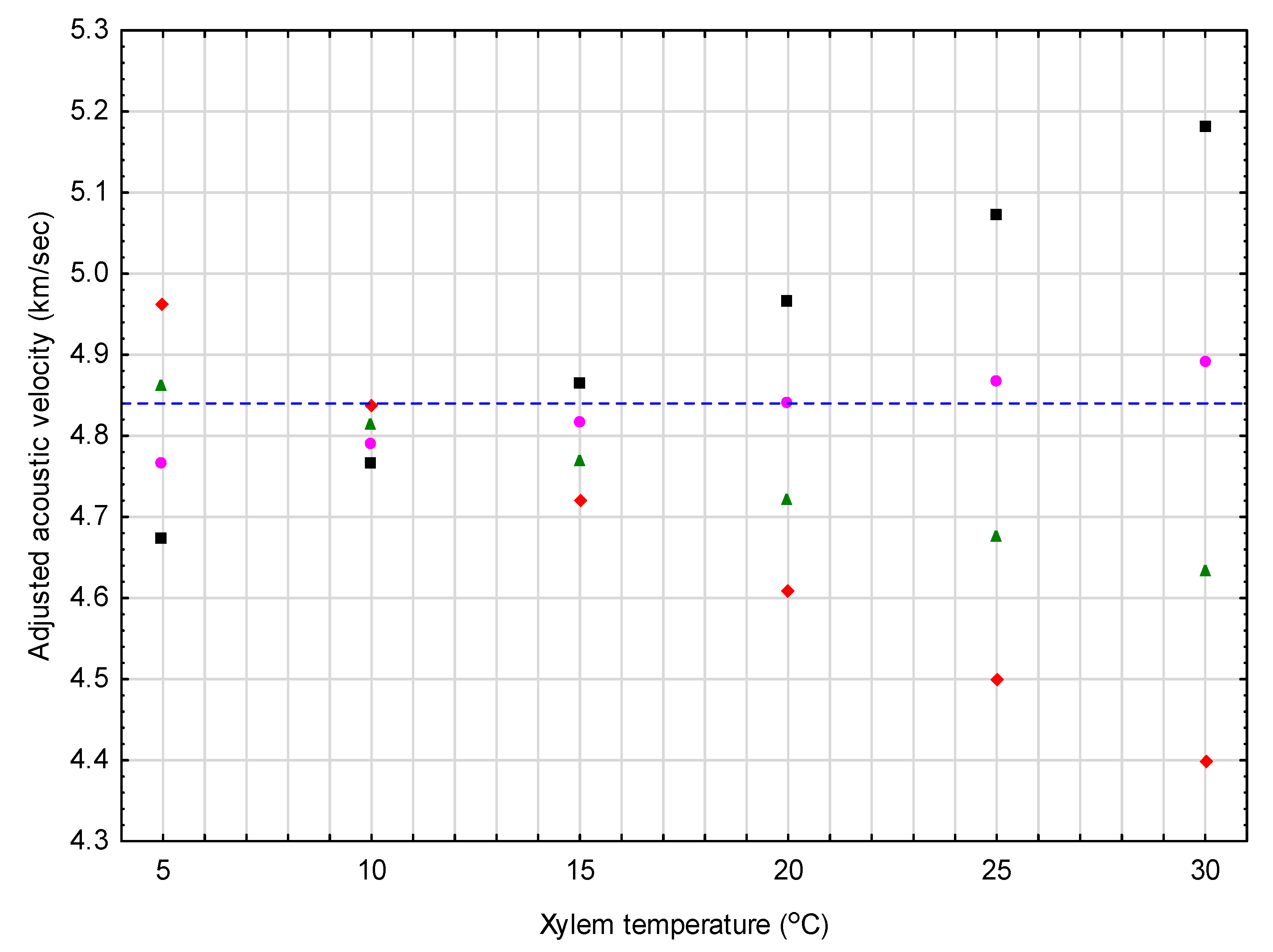
Figure 1 and Figure 2 exemplify the resultant correction equations developed for red pine and jack pine, respectively. Specifically, Figure 1 provides adjusted acoustic velocity estimates for a conceptually representative red pine tree, for which the velocity was set at a 4.84 km/s value (mean value of the selected red pine sample trees used to obtain the ${\overline{v}}_{d(..k;t_x=20,m_x=40)}$ value) across 24 different moisture and temperature conditions (i.e., 4 moisture levels (30%, 35%, 40%, and 45%) × 6 temperatures (5 °C, 10 °C, 15 °C, 20 °C, 25 °C, and 30 °C)). The percentage adjustments for the example cases shown, ranged from −2.5% at the lowest temperature (5 °C) to +9.1% at the highest temperature (30 °C) for the lowest moisture level considered (30%). For the highest moisture level considered (45%), the percentage adjustment ranged from +3.5% at the lowest temperature (5 °C) to −7.1% at the highest temperature (30 °C). More importantly, however, within the context of the operable range of v_d values observed for the red pine sample trees (0.80 km/s; minimum of 4.49 to a maximum of 5.29 km/s), these percentage changes increase consequentially: (1) To −15.3% at 5 °C and +55.2% at 30 °C, for a mean moisture level of 30%; and (2) to +20.9% at 5 °C and −42.7% at 30 °C, for a mean moisture level of 45%.

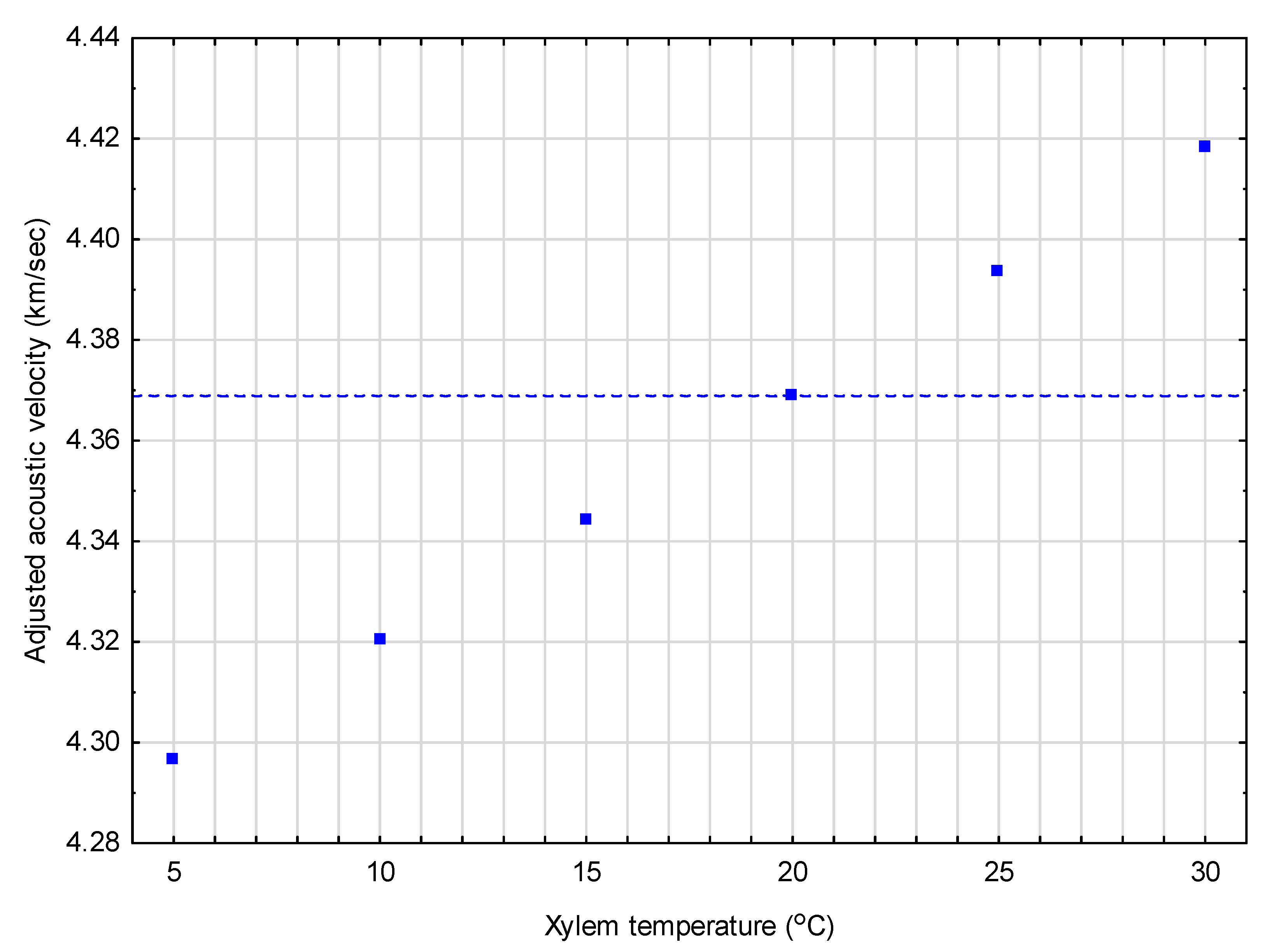
Similar to Figure 1, Figure 2 provides adjusted acoustic velocity estimates for a conceptually representative jack pine tree, for which the velocity was set at a 4.37 km/s value (mean of the selected jack pine sample trees used to obtain the ${\overline{v}}_{d(..k;t_x=20)}$ value), across 6 temperatures (5, 10, 15, 20, 25, and 30 °C)). On a percentage basis, the magnitude of the adjustment ranged from +1.7% at the lowest temperature (5 °C) to −1.1% at the highest temperature (30 °C). However, within the context of the operable range of v_d values observed for the jack pine sample trees (0.85 km/s; minimum of 4.01 to a maximum of 4.86 km/s), these percentage changes also increase substantially: To +8.5% at 5 °C and −5.8% at 30 °C.

4. Discussion

The primary objective of this study was to investigate the significance of xylem moisture effects on the relationship between acoustic velocity and xylem temperature within standing red pine and jack pine trees. Deploying an empirical-based sampling approach, consisting of replicated measurements of v_d within the same set of plantation grown red pine and jack pine trees throughout the spring-to-autumn seasonal period, during which t_x and m_x varied naturally, combined with the subsequent statistical-based analytics involving the application of hierarchical, mixed-effects regression models, yielded statistically validated regression models. Specifically, the final model specifications were (1) comprised of only significant (p ≤ 0.05) dependent variables with the appropriate fixed and (or) and random effects included, (2) compliant with the underlying homogenous variance and independence statistical assumptions, (3) adequate in terms of the magnitude of v_d variation explained (64% for red pine and 90% for jack pine), (4) devoid of consequential evidence of systematic lack-of-fit issues, and (5) adequate in terms of predictive precision (e.g., absolute tolerance intervals indicated that 95% of the expected errors generated using the parameterized functions would fall within ±0.17 km/s (red pine) and ±0.11 km/s (jack pine) of their true value, 95% of the time).

Functionally, the v_d–t_x relationship for red pine significantly (p ≤ 0.05) varied in a complex and systematic fashion with xylem moisture: v_d increased with increasing t_x at lower mean moisture levels (<38%) but conversely decreased with increasing t_x at higher mean moisture levels (>38%). More generally, the v_d–t_x relationship was directly proportional at the lower moisture levels, with the slope of relationship increasing in value with decreasing wood moisture, indicating that acoustic velocity was more sensitive to changes in temperature as moisture levels declined. For example, at lower moisture levels, acoustic velocity would increase by approximately 0.01 km/s for every 1 °C increase in temperature when moisture was 35% (${\beta }_{10}+{\beta }_{11}{\overline{m}}_x$, where ${\overline{m}}_x$ = 35 yields + 0.0096; Table 2), versus 0.02 km/s for every 1 °C increase in temperature when moisture was 30% (${\beta }_{10}+{\beta }_{11}{\overline{m}}_x$, where ${\overline{m}}_x$ = 30 yields + 0.0242; Table 2). Conversely, the v_d–t_x relationship was inversely proportional at the higher moisture levels, with the slope of relationship declining in value with increasing wood moisture, suggesting that acoustic velocity was more sensitive to changes in temperature as moisture levels increased. For example, at higher moisture levels, acoustic velocity would decrease by approximately 0.01 km/s for every 1 °C increase in temperature when moisture was 40% (i.e., ${\beta }_{10}+{\beta }_{11}{\overline{m}}_x$, where ${\overline{m}}_x$= 40 yields − 0.0050; Table 2), versus a decrease of approximately 0.02 km/s for every 1 °C increase in temperature when moisture was 45% (${\beta }_{10}+{\beta }_{11}{\overline{m}}_x$, where ${\overline{m}}_x$ = 45 yields − 0.0050; Table 2). The threshold moisture value at which the v_d–t_x relationships switched from directly proportional to inversely proportional was approximately 38.3% (i.e., ${\beta }_{10}/{\beta }_{11}$; Table 2). Conversely, the v_d–t_x relationship for jack pine was not significantly (p ≤ 0.05) influenced by xylem moisture levels. The v_d–t_x relationship was inversely proportional, with a constant slope across the temperature spectrum examined (i.e., −0.0049; Table 2). Empirically, this slope value indicates that acoustic velocity would decline by approximately 0.01 km/s for every 1 °C increase in xylem temperature.

Given these analytical findings, that is, significant (p ≤ 0.05) relationships between v_d and t_x for both species, and the associated moderation effect of xylem moisture on the v_d–t_x relationship within red pine stems, dictated the realization of the study’s secondary objective: The development of correction models. Specifically, based on the final species-specific hierarchical model specifications, corresponding correction equations were developed for (1) adjusting observed acoustic velocity values measured at a specific xylem temperature of t_x and moisture value of m_x on a red pine tree ($v_{d(t_x,m_x)}$) to corresponding acoustic velocity equivalents referenced to standardized temperature (20 °C) and moisture (40%) conditions ($v_{d(t_x=20,m_x=40)}$) and (2) adjusting observed acoustic velocity values measured at a specific xylem temperature of t_x on a jack pine tree ($v_{d(t_x)}$) to corresponding acoustic velocity equivalents referenced to a standardized temperature (20 °C) ($v_{d(t_x=20)}$). Based on the range of xylem temperatures (≈5 °C–30 °C) and mean xylem moisture levels (≈30–45%) observed within the sample tree population throughout the spring-to-autumn seasonal period, the magnitude of the average adjustment required would be in the order of 0.12 km/s for red pine and 0.04 km/s for jack pine.

Although the decision to deploy the correction equations would be governed by the precision requirements of the acoustic sampler, it is noteworthy to consider the magnitude of these adjustments when expressed as percentage of the sample range of acoustic velocities observed across the sampling events. For example, for red pine, the operable range of v_d values was approximately 0.80 km/s (from a minimum of 4.49 to a maximum of 5.29 km/s), and hence the mean relative adjustment required would be in the order of 15%. More precisely, however, when calculating adjustment values for specific temperature and moisture conditions, the percentage adjustments increase consequentially: For example, (1) −15.3% at 5 °C and +55.2% at 30 °C for a moisture level of 30%; and (2) to +20.9% at 5 °C and −42.7% at 30 °C for a moisture level of 45%. Similarly, for jack pine, the operable range of v_d values was approximately 0.85 km/s (from a minimum of 4.01 to a maximum of 4.86 km/s), and hence the mean relative adjustment required would be in the order of 5%. Likewise, however, the relative adjustment within the context of the operable range of v_d values would not be as dramatic as that for red pine but would still increase by +8.5% at 5 °C and −5.8% at 30 °C. Again, while the decision to implement the correction equations when acoustic sampling is ultimately related to the precision requirements of the end-user, these percentage-based results nevertheless illustrate the potential operational importance of their deployment when sampling; particularly during conditions in which xylem temperature and moisture levels approach the extremities of their spring-to-autumn seasonal ranges.

Acoustic-based methods belong to a broader suite of evolving technologies that can assist the forest management and research communities in the non-destructive estimation of internal wood quality characteristics (see [28] for a comprehensive summary). Briefly, in addition to acoustic-based approaches for estimating the dynamic modulus of elasticity, wood density, microfibrial angle, cell wall thickness, fiber coarseness, and specific surface area within standing trees via time-of-flight tools (e.g., Director ST300 (Fibre-gen Inc.); [7]) or within harvested logs via resonance instruments (Hitman ST200 (Fibre-gen Inc.); [29]), these innovative technologies include (1) mechanical-based physical resistance measures for wood density estimation via amplitude metrics derived from micro-drill resistance profiles (e.g., Resistograph micro-drill tool (IML, Inc., Moultonborough, NH, USA); [7,30]) or penetration measures arising from impact tools (e.g., Pilodyn impact device [31]), and (2) electromagnetic-based, near-infrared spectroscopic methods for estimating wood density, microfibrial angle, modulus of elasticity, and cell wall thickness (e.g., [32]).

In reference to the acoustic approaches, it is noteworthy to appreciate that the relationship between acoustic velocity and the dynamic modulus of elasticity for standing trees is different from that specified for harvested logs. The latter relationship employs the velocity of a mechanically induced longitudinal stress wave, rather than the velocity of a mechanically induced dilatational or quasi-dilatational stress wave which is measured within standing tree stems [33]. Although the wave types differ, along with their functional relationships with the dynamic modulus of elasticity, the two wave velocities have shown to be empirically correlated with each other for a number of coniferous species including Sitka spruce (Picea sitchensis (Bong.) Carr.), western hemlock (Tsuga heterophylla (Raf.) Sarg), jack pine, ponderosa pine (Pinus ponderosa Dougl. ex Laws.), radiata pine (Pinus radiata D. Don), and red pine ([7,8,34]). This degree of concordance between the velocity measures within standing trees, and those within derived logs across multiple species, provides a measure of confirmatory support for acoustic-based estimation of internal wood fiber attributes.

The application of the acoustic approach, in terms of forecasting wood stiffness and other commercially-relevant attributes, could result in more precise prediction of end-product potential during pre-harvest assessments and surveys. These predictions could be used to inform segregation decision-making, and thus potentially contribute to increased allocation efficiencies along the upstream portion of the forest products supply chain. Similarly, fiber attribute predictions derived from validated acoustic-based relationships could be more widely employed as indirect surrogate measures of wood quality within silvicultural research studies. Overall, the acoustic approach represents an efficient economic alterative to the logistically challenging and expensive destructive methods used to determine commercially relevant fiber attributes (e.g., Silviscan [35]). Although these presuppositions highlight the positive potentials of the acoustic approach, its ultimate deployment will be largely dependent on the precision requirements and associated error tolerances of the end-user.

The empirical results reported to date have been largely supportive of the acoustic approach in terms of the statistical significance of the fiber prediction relationships. However, the degree of variation among the studies in terms of exploratory power (percentage of variation explained) and predictive ability (precision) suggest improvements may be required if attaining precise point-estimates of stiffness are required. For example, with respect to results reported for red pine [7] and jack pine [8], the m_e–v_d relationships were both statistically significant at the 0.05 probability level, explained 42% (red pine) and 71% (jack pine) of the variation in m_e, and were able to provide point estimates at an expected precision level of approximately ±1.5 GPa (red pine) and ±2.7 GPa (jack pine). Operationally, however, even when assuming that the standing tree m_e estimate would be approximately equal to its static counterpart within a derived solid wood end-product (e.g., dimensional lumber), the acoustic-based estimates would not be precise enough to sort standing trees into NLGA (National Lumber Grades Authority)-based grade classes, given that their classes differ by an average of only ±0.7 GPa (Table 2 in the NLGA grading guidelines ([36])). Collectively, these results and associated inferences suggest that identifying and accounting for consequential sources of variation could be advantageous to advancing the acoustic approach in both forest operations and silvicultural research.

Accordingly, this study concentrated on investigating the significance of two of the most important known sources of acoustic velocity variation, as previously identified in the literature: Xylem temperature and xylem moisture (e.g., [9,10,11,12,37]). These previous studies have revealed a range of consequential effects particularly in terms of those arising from temperature variation. Similar to this study, analytical solutions, via the provision of correction or adjustment equations, have also been derived from these analyses. Overall, the consequences of the effects are most concerning when xylem moistures fall below fiber saturation thresholds, or when xylem temperatures fall below the freezing point (0 °C). Published results most pertinent to this study are those provided by Gao et al. [10], who investigated temperature effects on standing red pine trees. Their findings, based on acoustic velocity and temperature sampling of 20 red pine trees throughout a full year, combined with the deployment of a segmented linear regression model, revealed that acoustic velocity decreased linearly by approximately 0.007 km/s for every 1 °C increase in ambient air temperature across a 0 °C to 30 °C range. This rate of change is in accordance with that reported here for red pine (e.g., decline of 0.005 km/s per 1 °C increase at 40% xylem moisture; Table 2) and jack pine (decline of 0.005 km/s per 1 °C increase; Table 2).

Although assessing other more correlative-based sources of variation, such as tree-to-tree acoustic velocity variation arising from growth-induced differences in wood structure, would be of utility (e.g., [38]), focusing on the underlying known causal sources, such as xylem temperature and moisture, was a logical first step. Furthermore, the provision of species-specific correction equations, which accounted for such variation, should contribute to minimizing the effects of environmental variability on the precision of acoustic-derived estimates of commercially relevant fiber attributes when deploying the acoustic approach.

5. Conclusions

The relationship between the dynamic modulus of elasticity of xylem tissue and acoustic velocity has been established for a number of commercially important coniferous species. However, results from previous investigations suggest the relationship may be effected by xylem temperature and moisture variation. Consequently, this study investigated the significance of these effects on acoustic velocity measurements within standing red pine and jack pine trees through (1) temporal and repeated sampling of the same set of red pine and jack pine sample trees throughout the spring-to-autumn seasonal period, and (2), given (1), statistical inference of the derived species-specific, statistically validated, hierarchical, linear, mixed-effects regression models. The results indicated that acoustic velocity was influenced by temperature for both species, whereas the influence of moisture was only observed for red pine. Resultantly, species-specific correction equations for adjusting observed acoustic velocity measurements to corresponding equivalents referenced to standardized temperature and moisture conditions were developed. Although the spatial concentration of the sample sites with respect to the species geographic ranges, along with the limited sample sizes, suggest that caution should be exercised when drawing conclusive statistical inferences or deploying the derived relationships outside of the study region, this study has demonstrated the consequential effects of environmental variability on acoustic velocity measures. Furthermore, the provision of quantitative solutions for accounting for these effects should be of utility when deploying the acoustic approach in forest operations and silvicultural research.

References

- Rowe, J.S. Forest Regions of Canada; Publication No. 1300; Government of Canada, Department of Environment, Canadian Forestry Service: Ottawa, ON, Canada, 1972.
- Zhang, S.Y.; Koubaa, A. Softwoods of Eastern Canada: Their Silvics, Characteristics, Manufacturing and End-Uses; Special Publication SP-526E; FPInnovations: Quebec City, QC, Canada, 2008. [Google Scholar]
- Ross, R.J. Nondestructive Evaluation of Wood, 2nd ed.; General Technical Report FPL-GTR-238; USDA, Forest Service, Forest Products Laboratory: Madison, WI, USA, 2015; p. 169.
- National Lumber Grades Authority (NLGA). Standard Grading Rules for Canadian Lumber; NLGA: Surrey, BC, Canada, 2014; p. 316.
- Hong, Z.; Fries, A.; Lunqvist, S.-O.; Gull, B.A.; Wu, H.X. Measuring stiffness using acoustic tool for Scots pine breeding selection. Scand. J. For. Res. 2015, 30, 363–372. [Google Scholar] [CrossRef]
- Mora, C.R.; Schimleck, L.R.; Isik, F.; Mahon, J.M.; Clark, A.; Daniels, R.F. Relationships between acoustic variables and different measures of stiffness in standing Pinus taeda trees. Can. J. For. Res. 2009, 39, 1421–1429. [Google Scholar] [CrossRef]
- Newton, P.F. Acoustic-based non-destructive estimation of wood quality attributes within standing red pine trees. Forests 2017, 8, 380. [Google Scholar] [CrossRef]
- Newton, P.F. In-forest acoustic-based prediction of commercially-relevant wood quality attributes within standing jack pine trees. For. Chron. 2018. submitted. [Google Scholar]
- Gao, S.; Wang, X.; Wang, L.; Allisson, R.B. Effect of temperature on acoustic evaluation of standing trees and logs: Part 1—Laboratory investigations. Wood Fiber Sci. 2012, 44, 286–297. [Google Scholar]
- Gao, S.; Wang, X.; Wang, L.; Allisson, R.B. Effect of temperature on acoustic evaluation of standing trees and logs: Part 2: Field investigation. Wood Fiber Sci. 2013, 45, 15–25. [Google Scholar]
- Moreno-Chan, J.; Walker, J.C.; Raymond, C.A. Effects of moisture content and temperature on acoustic velocity and dynamic MOE of radiata pine sapwood boards. Wood Sci. Technol. 2010, 4, 609–626. [Google Scholar] [CrossRef]
- Llana, F.L.; Iñiguez-Gonzalez, G.; Martitegui, A.; Niemz, P. Influence of temperature and moisture content on non-destructive measurements in Scots pine wood. Wood Res. 2014, 59, 769–780. [Google Scholar]
- Llana, D.F.; Íñiguez-González, G.; Martínez, R.D. Influence of timber moisture content on wave time-of-flight and longitudinal natural frequency in coniferous species for different instruments. Holzforschung 2018, 72, 405–411. [Google Scholar] [CrossRef] [Green Version]
- Unterwieser, H.; Schickhofer, G. Influence of temperature and moisture content on the dynamic properties of ungraded spruce boards. Eur. J. Wood Prod. 2012, 70, 629–638. [Google Scholar] [CrossRef]
- Carter, P.; Briggs, D.; Ross, R.J.; Wang, X. Acoustic testing to enhance western forest values and meet customer wood quality needs. In Productivity of Western Forests: A Forest Products Focus; Harrington, C.A., Schoenholtz, S.H., Eds.; Gen. Tech. Rep. PNW-GTR-642; USDA, Forest Service, Pacific Northwest Research Station: Portland, OR, USA, 2005; pp. 121–129. [Google Scholar]
- Wang, X.; Carter, P.; Ross, R.J.; Brashaw, B.K. Acoustic assessment of wood quality of raw materials: A path to increased profitability. For. Prod. J. 2007, 57, 6–14. [Google Scholar]
- Filipescu, C.N.; Trofymow, J.A.; Koppenaal, R.S. Late-rotation nitrogen fertilization of douglas-fir: Growth response and fibre properties. Can. J. For. Res. 2017, 47, 134–138. [Google Scholar] [CrossRef]
- Lenz, P.; Auty, D.; Achim, A.; Beaulieu, J.; Mackay, J. Genetic improvement of white spruce mechanical wood traits—Early screening by means of acoustic velocity. Forests 2013, 4, 575–594. [Google Scholar] [CrossRef]
- Beckwith, A.F.; Roebbelen, P.; Smith, V.G. Red Pine Plantation Growth and Yield Tables; Forest Research Report No. 108; Ontario Ministry of Natural Resources; Ontario Tree Improvement and Forest Biomass Institute: Maple, ON, Canada, 1983.
- Carmean, W.H.; Niznowski, G.P.; Hazenberg, G. Polymorphic site index curves for jack pine in Northern Ontario. For. Chron. 2001, 77, 141–150. [Google Scholar] [CrossRef] [Green Version]
- Wilson, F.G. Numerical expression of stocking in term of height. J. For. 1946, 44, 758–761. [Google Scholar]
- Raudenbush, S.W.; Bryk, A.S. Hierarchical Linear Models: Applications and Data Analysis Methods, 2nd ed.; Sage: Newbury Park, CA, USA, 2002; p. 485. [Google Scholar]
- Raudenbush, S.W.; Bryk, A.S.; Cheong, Y.F.; Congdon, R.T.; Toit, M., Jr. HLM 7—Hierarchical Linear and Nonlinear Modeling; Scientific Software International Inc.: Lincolnwood, IL, USA, 2011; p. 360. [Google Scholar]
- Ek, A.R.; Monserud, R.A. Performance and comparison of stand growth models based on individual tree and diameter-class growth. Can. J. For. Res. 1979, 9, 231–244. [Google Scholar] [CrossRef]
- Reynolds, M.R., Jr. Estimating the error in model predictions. For. Sci. 1984, 30, 454–469. [Google Scholar]
- Gribko, L.S.; Wiant, H.V., Jr. A SAS template program for the accuracy test. Compiler 1992, 10, 48–51. [Google Scholar]
- Gujarati, D.N. Essential of Econometrics, 3rd ed.; McGraw-Hill/Irwin Inc.: New York, NY, USA, 2006; p. 553. [Google Scholar]
- Rudnicki, M.; Wang, X.; Ross, R.J.; Allison, R.B.; Perzynski, K. Measuring Wood Quality in Standing Trees: A Review; General Technical Report FPL–GTR–248; USDA, Forest Service, Forest Products Laboratory: Madison, WI, USA, 2017; p. 11.
- Newton, P.F. Predictive relationships between acoustic velocity and wood quality attributes for red pine logs. For. Sci. 2017, 63, 504–517. [Google Scholar] [CrossRef]
- Rinn, F.; Schweingruber, R.H.; Schär, E. Resistograph and X-ray density charts of wood: Comparative evaluation of drill resistance profiles and X-ray density charts of different wood species. Holzforschung 1996, 50, 303–311. [Google Scholar] [CrossRef]
- Wu, S.J.; Xu, J.M.; Li, G.Y.; Risto, V.; Lu, Z.H.; Li, B.Q.; Wang, W. Use of the pilodyn for assessing wood properties in standing trees of Eucalyptus clones. J. For. Res. 2010, 21, 68–72. [Google Scholar] [CrossRef] [Green Version]
- Tsuchikawa, S.; Kobori, H. A review of recent application of near infrared spectroscopy to wood science and technology. J. Wood Sci. 2015, 61, 213–220. [Google Scholar] [CrossRef] [Green Version]
- Wang, X.; Carter, P. Acoustic assessment of wood quality in trees and logs. In Nondestructive Evaluation of Wood, 2nd ed.; General Technical Report FPL-GTR-238; Ross, R.J., Ed.; USDA, Forest Service, Forest Products Laboratory: Madison, WI, USA, 2015; pp. 87–102. [Google Scholar]
- Wang, X.; Ross, R.J.; Carter, P. Acoustic evaluation of wood quality in standing trees. Part I. Acoustic wave behavior. Wood Fiber Sci. 2007, 39, 28–38. [Google Scholar]
- Defo, M.; Goodison, A.; Nelson, U. A method to map within-tree distribution of fibre properties using SilviScan-3 data. For. Chron. 2009, 85, 409–414. [Google Scholar] [CrossRef] [Green Version]
- National Lumber Grades Authority (NLGA). Special Products Standard for Machine Graded Lumber; NLGA: Surrey, BC, Canada, 2013; p. 40.
- Kang, H.; Booker, R.E. Variation of stress wave velocity with MC and temperature. Wood Sci. Technol. 2002, 36, 41–54. [Google Scholar] [CrossRef]
- Bérubé-Deschênes, A.; Franceschini, T.; Schneider, R. Factors affecting plantation grown white spruce (Picea glauca) acoustic velocity. J. For. 2016, 114, 629–637. [Google Scholar] [CrossRef]
Figure 1.
Graphical exemplification of the results from the red pine correction equation (Equation (8a)) when adjusting a constant observed acoustic value of 4.84 km/s (denoted by horizontal dash-line) to standardized conditions (tx = 20 °C and mx = 40%) for 4 mean moisture classes (30%, 35%, 40%, and 45% as denoted by solid diamond, triangle, circle, and square symbols, respectively) across a 5 °C – 30 °C temperature range.
Figure 2.
Graphical exemplification of the results from the jack pine correction equation (Equation (8b)) when adjusting a constant observed acoustic value of 4.37 km/s (denoted by horizontal dash-line) to standardized conditions (tx = 20 °C) across a 5 °C–30 °C temperature range.